Abstract
Asset management is a process that deals with numerous types of data, including spatial and temporal data. Such an occurrence is attributed to the proliferation of information sources. However, the lack of a comprehensive asset data model that encompasses the management of both spatial and temporal data remains a challenge. Therefore, this paper proposes a graph-based spatio-temporal data model to integrate spatial and temporal information into asset management. In the spatial layer, we provide a graph-based method that uses topological containment and connectivity relationships to model the interior building space using data from 3D city models. In the temporal layer, we proposed the Aggregated Directly-Follows Multigraph (ADFM), a novel process model based on a directly-follows graph (DFG), to show the chronological flow of events in asset management by taking into consideration the repetitive nature of events in asset management. The integration of both layers allows spatial, temporal, and spatio-temporal queries to be made regarding information about events in asset management. This method offers a more straightforward query, which helps to eliminate duplicate and false query results when assessed and compared with a flattened graph event log. Finally, this paper provides information for the management of 3D spaces using a NoSQL graph database and the management of events and their temporal information through graph modelling.
1. Introduction
Asset management is a subset within the Architecture, Engineering, Construction, and Operation (AECO) [1] sector that is deeply involved in asset lifecycles. The primary objective of an asset lifecycle is to establish guidelines for the effective management of assets, from their acquisition to their eventual disposal. An asset lifecycle deals with numerous types of information to facilitate effective data-driven decision-making. Examples of such information include operational and maintenance (O&M) information, the spatial description of the assets, and historical information regarding assets in the O&M phase of an asset lifecycle. Effective management of this diverse range of information will allow asset managers to establish a methodical and active asset management strategy that focuses on predictive asset maintenance (PdM) [2].
According to the authors of [3], asset managers often struggle with the abundance of information rather than the lack of it. A contributing factor to this phenomenon is the proliferation of Big Data and its technologies, which have emerged as an indispensable source of information and information management for asset management [4]. Information management stands as a critical subject for asset managers when examining the optimal approach to managing the heterogeneous data sources involved in asset management. The increasing prevalence of digital asset management subsequently prompts information management as an emerging topic in asset management research, which results from the increasing prevalence of digital asset management. The digital and virtual transformation of asset management through the involvement of 3D models using the digital twinning approach could be the key to solving data storage and data processing while fully utilising rich information from various sources [5].
While having a wealth of information and data is advantageous for asset management decision support tools, managing them to ensure the quality of the information is often a challenge. Substandard information quality caused by inadequate information management will impose significant difficulties on asset management operations [6]. The resistance to implementing an efficient method for information management in asset management stems from the absence of a widely accepted method for managing information originating from multiple sources [7] and the interoperability issues of available data [1,7,8,9]. According to several studies, asset and facility management operations spend approximately 80% of their time searching for relevant information, a problem originating from inadequate data integration [10] and poor interoperability [1,11] that hinders effective decision-making. Therefore, it is imperative to address the issue of data interoperability in asset management with a well-defined strategy, which can be achieved through the development of a robust asset management data modelling approach [7,8].
Efficient operation in asset management relies on effective data exchange and sharing in all phases of the asset lifecycle [7,12]. A systematic review by the authors of [7] demonstrated several built environment data models that aim to solve the problems of interoperability and data exchange in the asset management domain. Data modelling in asset management can be regarded as a method to facilitate a seamless exchange of information by establishing the classification and relationship of entities, ontology, taxonomy, and information hierarchy of physical assets [8]. Designing and structuring are important aspects to consider when developing an asset data model [13]. This is because a data model that possesses a systematic conceptual and logical design is not only capable of facilitating the smooth flow of data but also grants the ability to integrate with a database to enhance the efficiency of data storage, data query, and data manipulation.
An essential consideration during the development of a data model is deciding which information must be incorporated to meet the operational requirements and demands of an asset-intensive organisation. In the context of infrastructure asset management, incorporating spatial information is crucial to constructing a reliable asset data model. Despite its prominence in asset management, the integration of spatial information into asset data models is seldom discussed. Spatial information is vital for risk management in asset management as it can be used to determine the hotspot of risk concerning infrastructure assets [14,15,16] and to assess the risk of exposure from natural disaster risks [17,18,19,20].
In asset management, specifically regarding building assets, spatial information comprises three distinct types of information, namely, coordinates, geometry, and space. Such information can be obtained using 3D city models, either by visualising them or are captured within the data structure of the 3D city models themselves. Building space arrangements within the buildings are classified as spatial information, which can be discerned through the visualisation of 3D city models. Incorporating the building space information into an asset data model could facilitate indoor navigation during a disaster risk, which is one of the capabilities of 3D city models when they are represented and modelled at a high level of detail (LoD) [21]. As an initial step towards developing an effective asset data model, a technique is required for modelling high-LoD 3D city models that manage to capture the arrangement of interior building spaces.
Asset management must also maintain records of temporal information in the form of historical data and the progression of events from the operation and maintenance phases of the asset lifecycle [22]. Temporal information plays a crucial role in making informed decisions in asset management [23] and improving the reliability of available assets [24]. Historical information can also provide valuable insights to diagnose problems with an asset, predict what will happen to an asset, and prescribe appropriate action for assets at risk [25]. Consequently, it is clear that asset management should incorporate temporal data and that providing strategies for managing temporal information is equally important.
Temporal information can be captured and managed using process mining techniques. Process mining is a discipline that facilitates the extraction of data regarding business processes from the event log information [26]. Asset management can benefit significantly from process mining techniques, which facilitate the discovery and modelling of event-related information including timestamps, activities, and their flows. Process mining identifies the flow of activity through the use of graphical representations.
The process mining domain plays a critical role in describing and analysing the flow of process events. Understanding the sequence of events in asset management is crucial for several reasons. Process mining techniques are designed to extract meaningful information from recorded event logs, which document various activities and interactions within an asset, and discover how the activities will affect asset performance. Therefore, by leveraging process mining, asset management organisations can significantly improve performance by analysing event sequences that can help enhance business processes [27,28]. Analysing the events helps to uncover inefficiencies and vulnerabilities that can aid risk assessment in asset management to prevent asset downtime.
This study aims to propose a comprehensive spatio-temporal asset data model that incorporates the aspects of building components from 3D city models and the management of events in the O&M phase of asset management. The proposed data model addresses two main gaps: the absence of a bi-dimensional data model in asset management and the insufficient focus on managing historical events within asset management.
2. Research Background
2.1. Asset Data Model
In the academic literature, asset data models are mainly discussed to support two main aspects. The first aspect concerns the discussion of asset data models to support the phases in asset management, predominantly the operation and maintenance (O&M) phases. Managing data in the O&M phase of asset management can be a challenging task as it deals with numerous data. The management of temporal information is also crucial during this phase, which focuses on managing historical data of various activities for prediction-based decision-making [11,13]. To manage the diverse information in asset management, Ref. [11] proposed a two-level semantic asset data model that divides the information based on their dynamicity characteristics. Meanwhile, Ref. [13] included historical information as one of the main entities in their data model. However, the primary issue is the lack of explanation regarding the management of historical data and their temporal attributes regarding asset-related activities. Assets that are subjected to the phases in the asset lifecycle will undergo multiple activities along their operational life. Therefore, it is vital to depict the flow of these activities so that asset managers can make personalised decisions based on specific asset conditions and be aware of the assets’ current state.
The second aspect is the discussion of asset data models to facilitate the enrichment of information and semantics with the aid of digital infrastructures such as GIS and building models, which are considered as spatial data. Such an aspect is motivated by the progression of asset management, which is transitioning towards digital asset management. Although data modelling is a well-known technique that has been implemented for decades, its lack of semantics is a noteworthy drawback [29]. There are examples of GIS and BIM integration being used to improve the semantics in the built cultural heritage domain. This integration allows for 3D modelling and the enrichment of semantic knowledge to enhance the documentation of built cultural heritage and improve information management and analysis [30,31]. Therefore, the lack of semantic knowledge in asset management can be overcome by incorporating data from external sources, including information from GIS and building models such as the Building Information Model (BIM) and City Information Model (CIM).
Digital infrastructures, such as GIS and multidimensional building models, are crucial for the digitalisation of asset management. Ref. [32] conducted a systematic literature review on the role of digital infrastructure for asset management and found that multidimensional (3D/4D) modelling such as the CIM is an advantageous asset management tool for managing managerial, technical, and financial data. Meanwhile, the GIS has been proven beneficial in geovisualization [33] and is needed to provide the spatial data and locations of assets in asset management via sensing and GPS technology [32]. Ref. [34] highlights the prevalent use of the GIS for infrastructure asset management due to its versatility and the fact that it is an established body of knowledge.
From the GIS perspective, both the GIS and the CIM are interrelated. The CIM is constructed from photogrammetry and laser scanning data obtained from GIS sources to generate the CIM, which is also referred to as 3D city models [35]. The 3D city models in the GIS are a component of the 3D GIS domain. The primary 3D city model formats in 3D GIS are CityGML and CityJSON, which can be distinguished mainly by their encoding. 3D city models have demonstrated their significance in numerous disciplines, such as urban planning, utilities, and asset management [36,37]. These semantically enriched 3D city models have advanced as an important decision support tool for many urban applications across numerous use cases [38]. Additionally, 3D city models serve as powerful tools in asset management that are primarily utilised for risk assessment [21,39,40,41].
Incorporating 3D city models as 3D spatial data into asset data models provides asset managers with an informative decision-making method by unlocking spatial analysis and spatial query. The progression towards digital asset management can be supported by incorporating 3D spatial data. However, the integration of 3D spatial data in asset management is rarely addressed within the asset data model framework. The 3D city models are equipped with intricate geometries and topologies [42] that provide hindrances to developing a comprehensive and efficient asset data model. Additionally, it is necessary to connect 3D spatial data with temporal information in asset management since temporal information is indispensable for making effective decisions in asset management [23,25]. Hence, there is a requirement for the efficient modelling of spatial, temporal, and spatio-temporal data to effectively manage this information in asset management practices.
2.2. Graph Data Model for Management of Events and Its Temporal Information
The flow and sequence of events across any domain can be depicted as a graph notion. Activities or events can be represented as nodes, while the flow of these activities and the relationships between them can be indicated using directed edges. Several process models have been developed and implemented to represent the flow of activity for business processes, such as BPMNs, Petri Nets, and DFGs [43]. The basis of process mining or the business process is the event log, which consists of activity and timestamp attributes [44] to describe the sequence of events [45]. Event logs in process mining are records of business processes that can provide further understanding of the performance of a process [46].
A Petri Net is a graphical and mathematical model that describes the interaction of processes within various applications, including business process modelling [47]. It is a bipartite directed graph that consists of two disjoint sets, namely, the places and transitions [28]. The edge or arc in a Petri Net connects places or transitions. Due to their characteristics as a bipartite graph, no two places or transition nodes can be connected using arcs. Meanwhile, a DFG is a directed graph to depict the sequence of events and the events that immediately follow a given event corresponding to a directly-follows (DF) relationship [43,44]. Finally, a BPMN is a process model language that combines several notations from the Unified Modelling Language (UML) and the XML Process Definition Language (XPDL) [47]. Although they are not formally regarded as graph models, BPMN models use nodes and edges to describe the flow and sequence between activities, which are the fundamentals of a graph.
Definition 1
(Event Logs) [46]. Given A is a set of activities, L is an event log, where t is a trace of activities such that = {a1, a2, a3,… an}, with .
Definition 2
(Petri Nets) [48]. A Petri Net is a 3-tuple N = (P, T, F), where
- 1.
- P and T are two disjoint finite sets called Places and Transitions, respectively.
- 2.
- is a set of directed edges called Flow.
Definition 3
(Directly-Follows Graph) [46]. Graph G = (N, E) is a Directly-Follows Graph (DFG), where
- 1.
- N is a set of nodes and E is a set of edges.
- 2.
- N = { | a is an activity recorded in at least one trace, t of the event log}.
- 3.
- E = {(x, y) | and there exists at least one trace, t where activity x is directly followed by activity y}.
The use of databases in the event log management of event logs within an organisation offers significant advantages, including the ability to customise queries to access a vast array of information [49]. Event data typically encompasses activities, identifiers, resources, event identification, and timestamps or other forms of attributes to state the sequence of events [22]. However, Ref. [47] emphasises that the majority of processes consist of numerous intricately interconnected entities, including activities, timestamps, activity identifiers, and other elements that offer deeper insights into any organisation’s process. This results in event data that comprises multidimensional information. Ref. [50] further adds that although relational databases possess the ability to manage multidimensional data, they do not have the proper ability to model and query the sequence of events. On the contrary, graph databases offer significant advantages when it comes to storing event processes that are presented through graph data models due to their benefits in storing, manipulating, and querying graph notations [51].
3. Spatio-Temporal Data Model
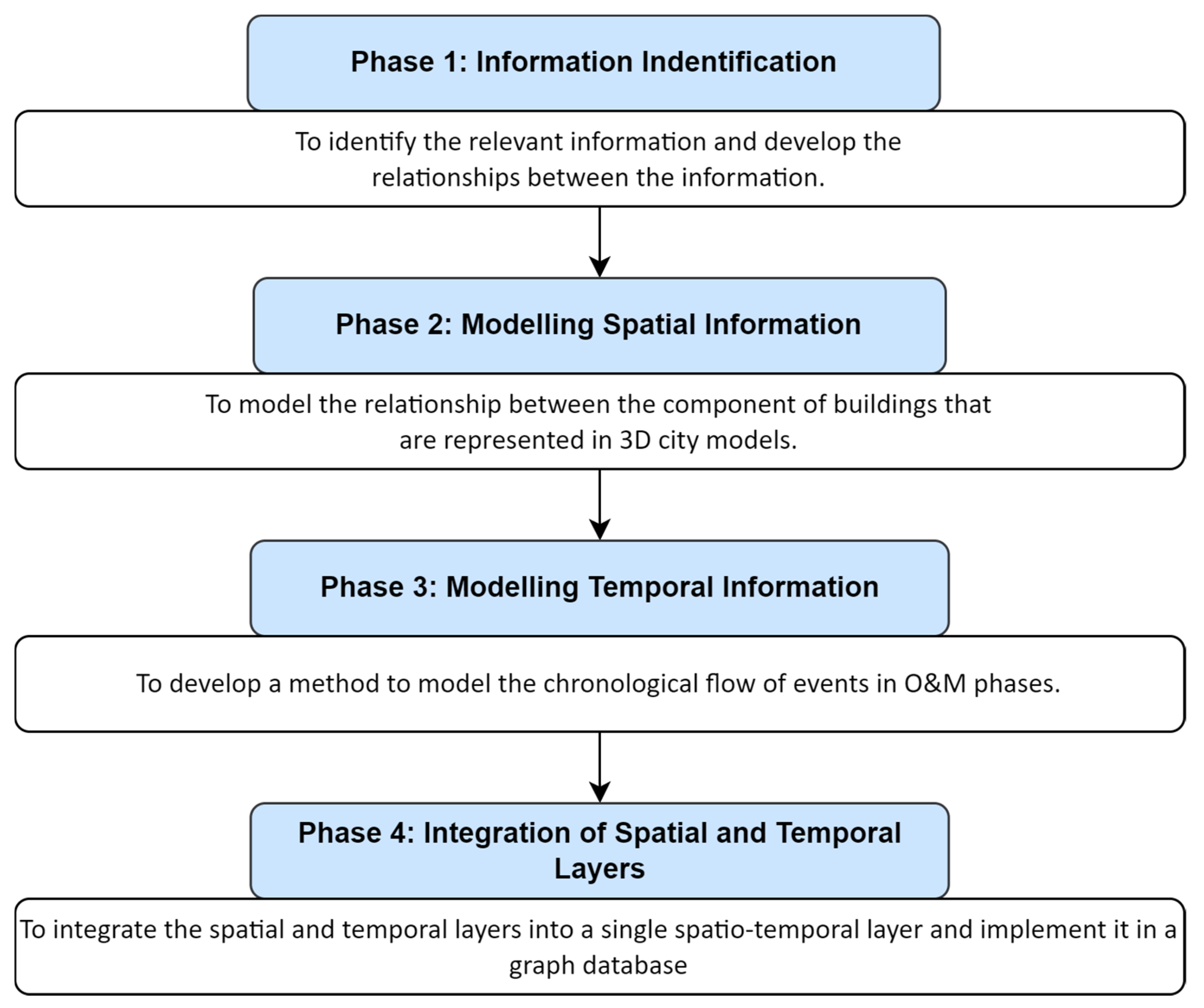
This section describes the methodology for developing an asset management spatio-temporal data model alongside the considerations for effective modelling of both spatial and temporal components in asset management. Figure 1 shows the four main phases of developing the data models, encompassing all the essential information required.
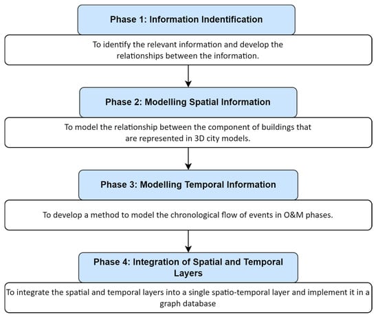
Figure 1.
Methodology of this study.
3.1. Phase 1: Information Identification
The development of data models is driven by the desire to standardise information originating from diverse sources. The primary aim of this paper is to establish a comprehensive representation of asset management information. Therefore, it is critical to ascertain the data necessary for asset management across the complete asset lifecycle. The information in asset management encompasses a wide range of categories, which can be captured by identifying the semantic properties of the assets. This will help to define the information, attributes, and relationships between the information and its corresponding attributes.
Several studies have been undertaken to determine the semantical data that are essential for the implementation of active asset management strategies through effective data management. The prominence of semantic information and attributes in asset management, along with their modelling and relationship definitions, has been established by a number of studies [11,13,52]. The findings suggest that information can be primarily classified as managerial and operational and maintenance (O&M) information. Managerial information is needed to assist the administration and management of assets, such as the asset manager, asset function, and asset specifications. Such information is commonly decided by the asset owner. On the other hand, O&M information is the key aspect in asset management to successfully operate the function of the assets. This includes the decision-making information, maintenance records, operational records, failure history, and other information pertinent to the O&M phase in the asset lifecycle. It is also a temporal layer that deals with temporal attributes, times, and events.
A common deficiency in the research is the exclusion of spatial data in asset data models. Failure to provide an explanation regarding the significance of spatial information in asset data model research could imply that this aspect of the model is not considered substantial. As explained in Section 2.1, a considerable body of research that is not centred on asset data models demonstrates that spatial information presented as 3D building models could benefit asset management. Therefore, this research will include spatial data in the form of a 3D city model alongside other previously mentioned categories of information, namely, managerial information and O&M information. Location, geometry, and space constitute the three additional components that comprise spatial information. Location data, also known as coordinates and geometry, are stored as attributes within the data structure of the 3D city model. Meanwhile, the spatial information provides a description of the building’s interior, including all building spaces like the floor level and rooms. However, information on the connections between interior building spaces is difficult to discern based solely on the encoding of 3D city models, such as CityJSON and CityGML. Nevertheless, the arrangement of the building’s interior is visible and can be easily validated when it is visualised using 3D city model visualisation tools. Figure 2 illustrates the categorisation of information in asset management.
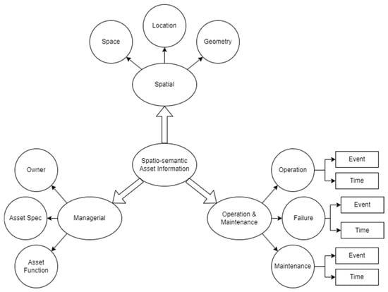
Figure 2.
Asset management information.
3.2. Modelling the Information
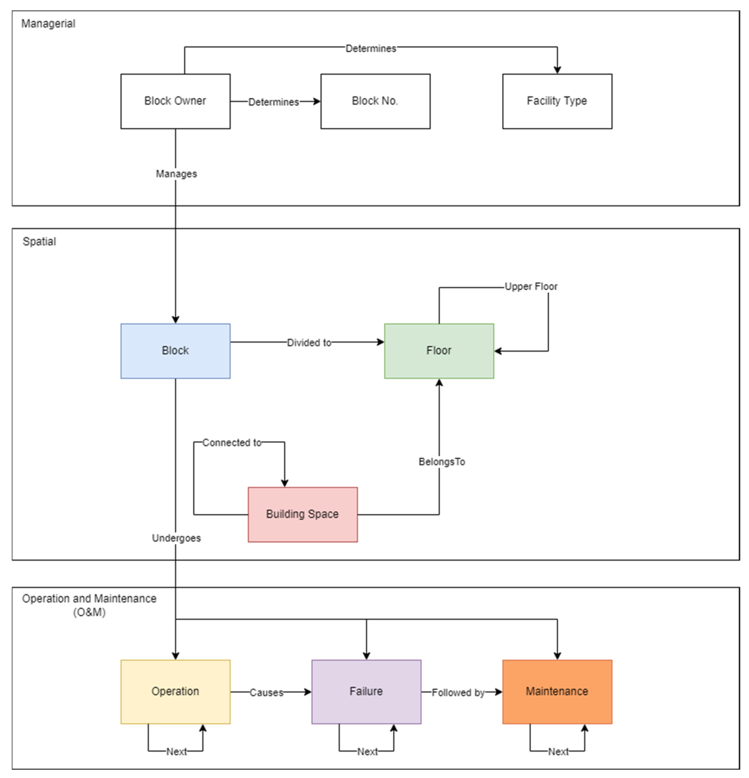
Figure 3 illustrates the correlation of data drawing upon the information uncovered in the previous sections. The depicted image can also be interpreted as a database schema, which is the initial phase in constructing a comprehensive data model for database implementation. The distinct classifications of information as shown in Figure 2 are treated as a separate layer (see Figure 3). The relationship between two elements of the same or different layer is indicated by the direction of the arrow. The primary categories of information discussed are the spatial and O&M layers as the information in these layers is integral for achieving the main objective of this study, which is to propose a spatio-temporal asset management data model.
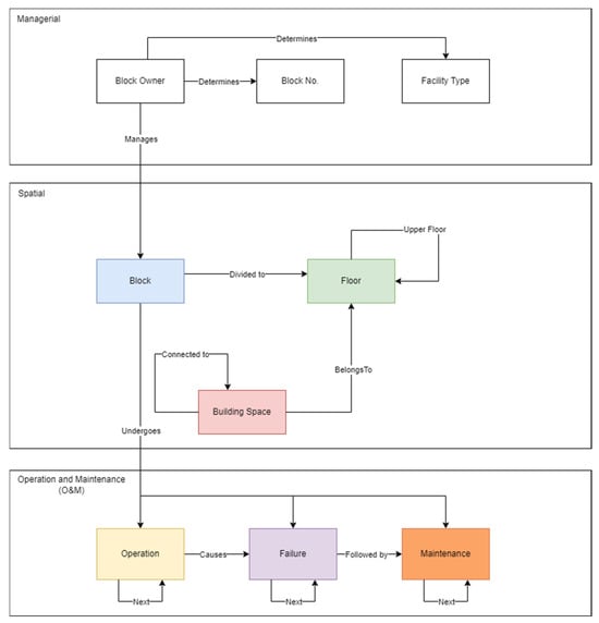
Figure 3.
Relationship between types of information for spatio-temporal asset management.
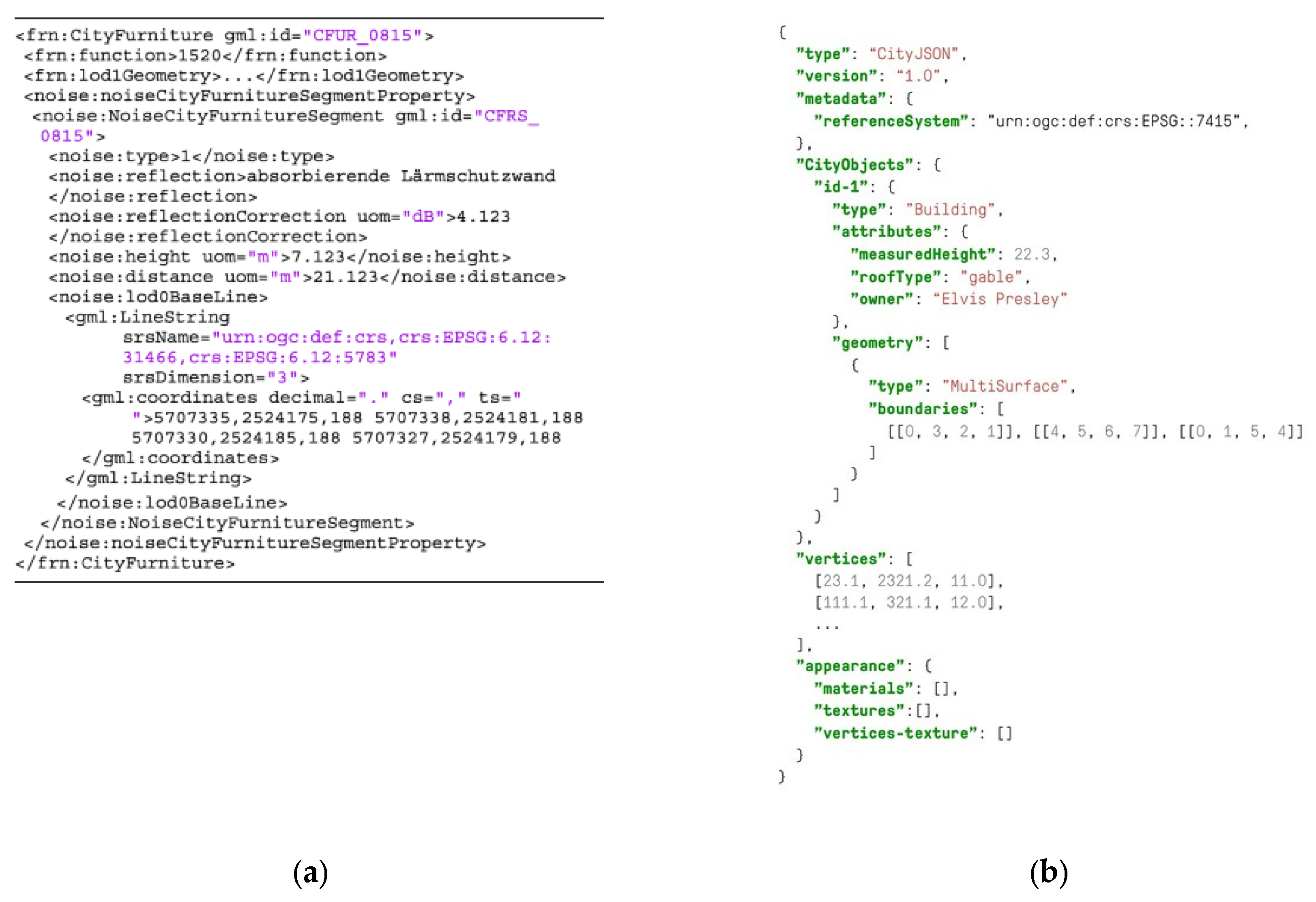
The spatial layer mainly concerns the interior building space elements (see Section 3.1) since it is treated as an independent attribute from the data structure of a 3D city model. Additional spatial components (i.e., geometry and location) are encapsulated within the data structure of a 3D city model. For example, CityGML and CityJSON, which are the 3D city model formats within the 3D GIS domain, are encoded in GML and JSON, respectively. They store both coordinates and geometry in their own encoding as illustrated by the example in Figure 4. Consequently, we aim to preserve this information within the 3D city model’s data structure without extracting it for inclusion in the data model. The modelling of interior building spaces aims to offer methods for modelling high-LoD 3D city models in any format. Three types of information are available in this layer, namely, the block, floor, and building spaces. As the primary entity, the block may be subdivided into its floors and the interior spaces of the buildings (see Figure 3). Whereas information in the O&M layer can be separated into operation, failure, and maintenance. This layer serves as the temporal layer of this data model, as it concerns managing the temporal attributes of times and events, as shown in Figure 2. Subsequently, the self-looping next relationship can be established to demonstrate the sequential and dynamic characteristics of the event information in this layer.
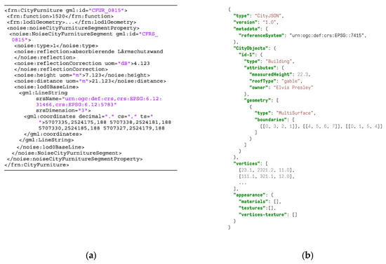
Figure 4.
Excerpt of (a) CityGML [53] and (b) CityJSON [54].
3.2.1. Phase 2: Modelling Spatial Information
A 3D building model was employed in this study to provide the spatial information necessary for determining the building space arrangement. This section explains how the 3D model was generated and used to model the spatial arrangement of the building.
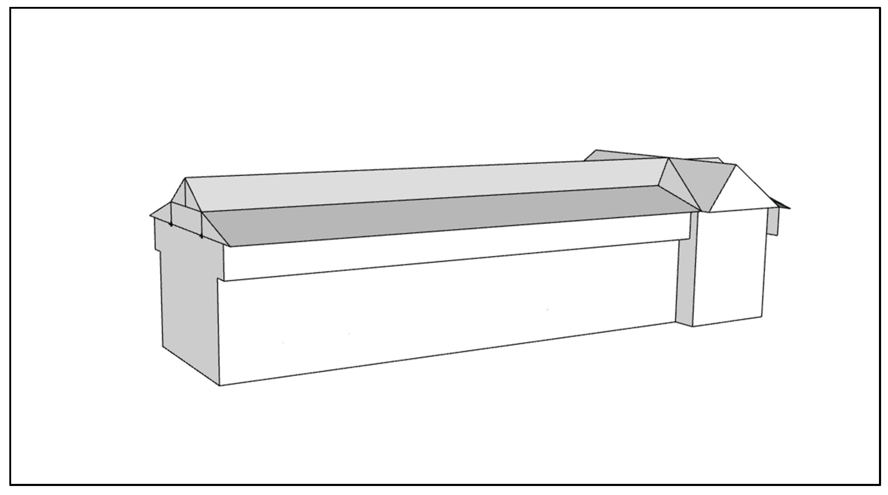
The 3D models were constructed using SketchUp 2023 (Version 23.1.340) software. Satellite images and aerial imagery of the structure were acquired prior to the development of the 3D models. The correct height and shape of the structure were extruded based on the data collected during site visits. Figure 5 shows the resultant 3D building model generated in SketchUp. It illustrates part of the building situated in Lingkaran Ilmu, Universiti Teknologi Malaysia (UTM), which was the research area of this study.

Figure 5.
3D Model generated in SketchUp.
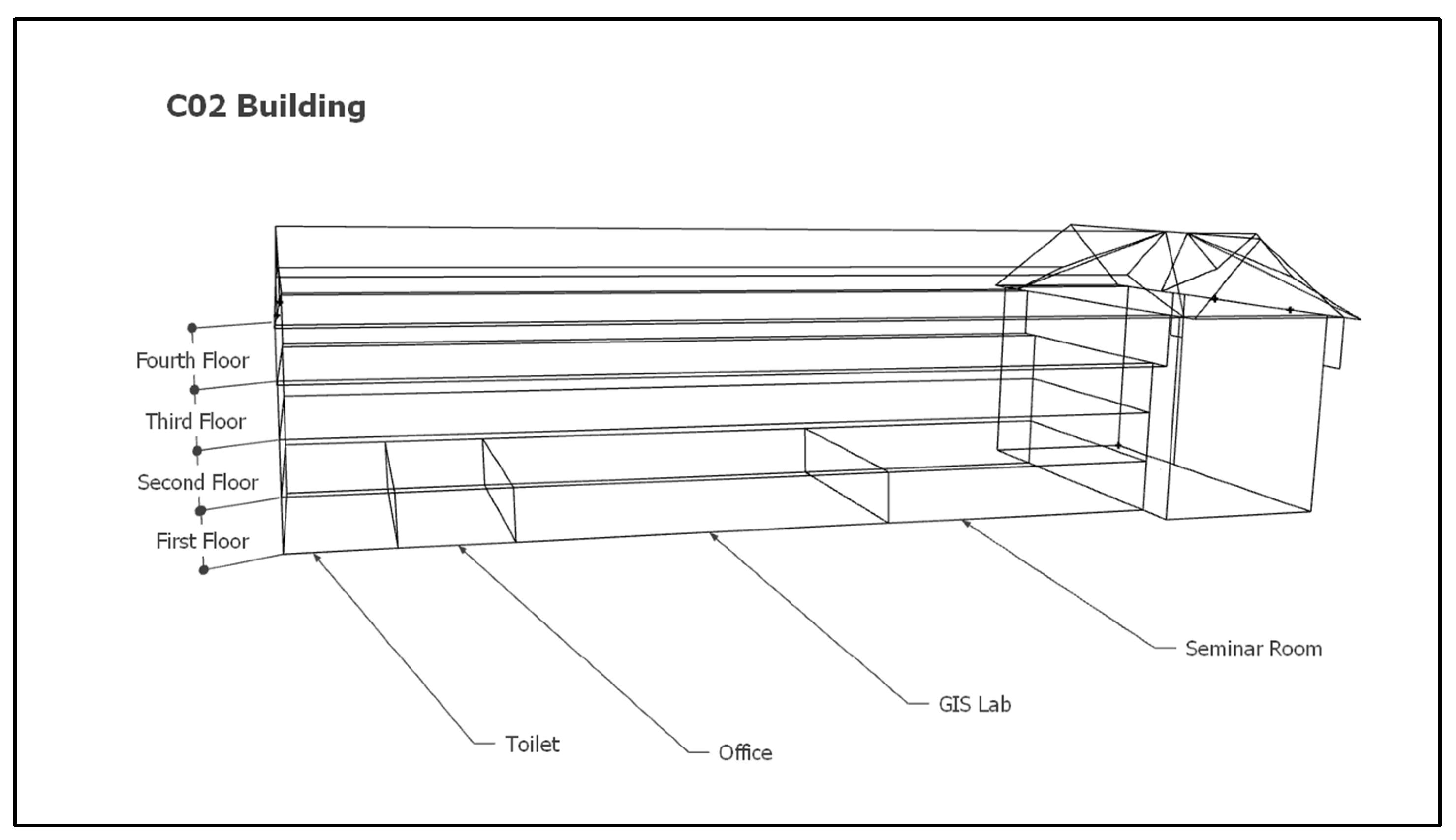
The model in Figure 5 is further improved by including individual floors and rooms within the C02 block to provide a more comprehensive representation of the interior building space of the structure, thereby enhancing the level of detail of the 3D model. Figure 6 shows a wireframe of the block to show how the floors and rooms are incorporated into the 3D model. This improvement significantly increases the level of detail required to simulate the buildings’ spatial arrangement, which will be beneficial when modelling the spatial data. Consequently, the buildings are separated into three levels, which are the block as the main entity, the floors within the block, and the individual rooms within each floor.

Figure 6.
Wireframe of the C02 block.
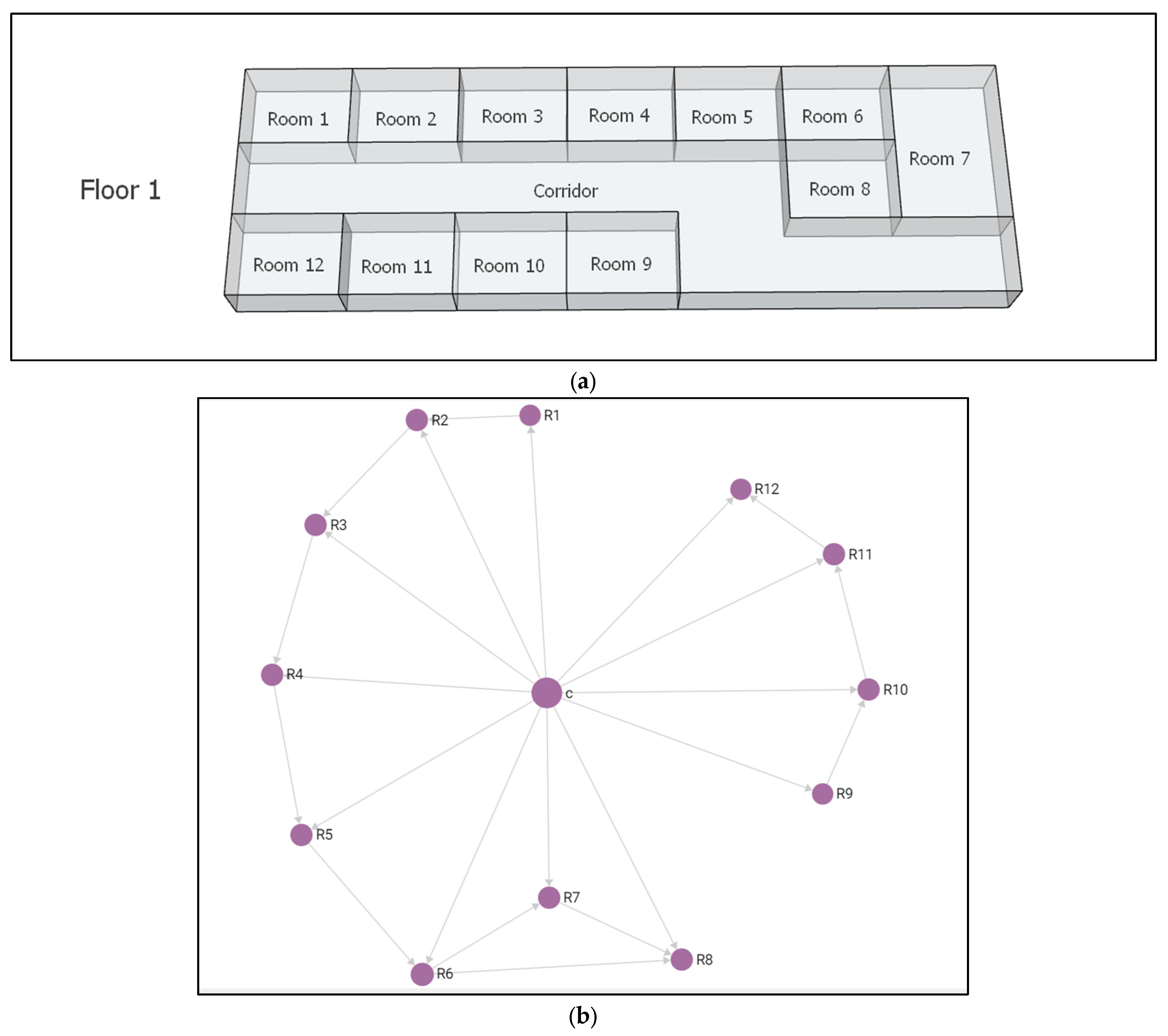
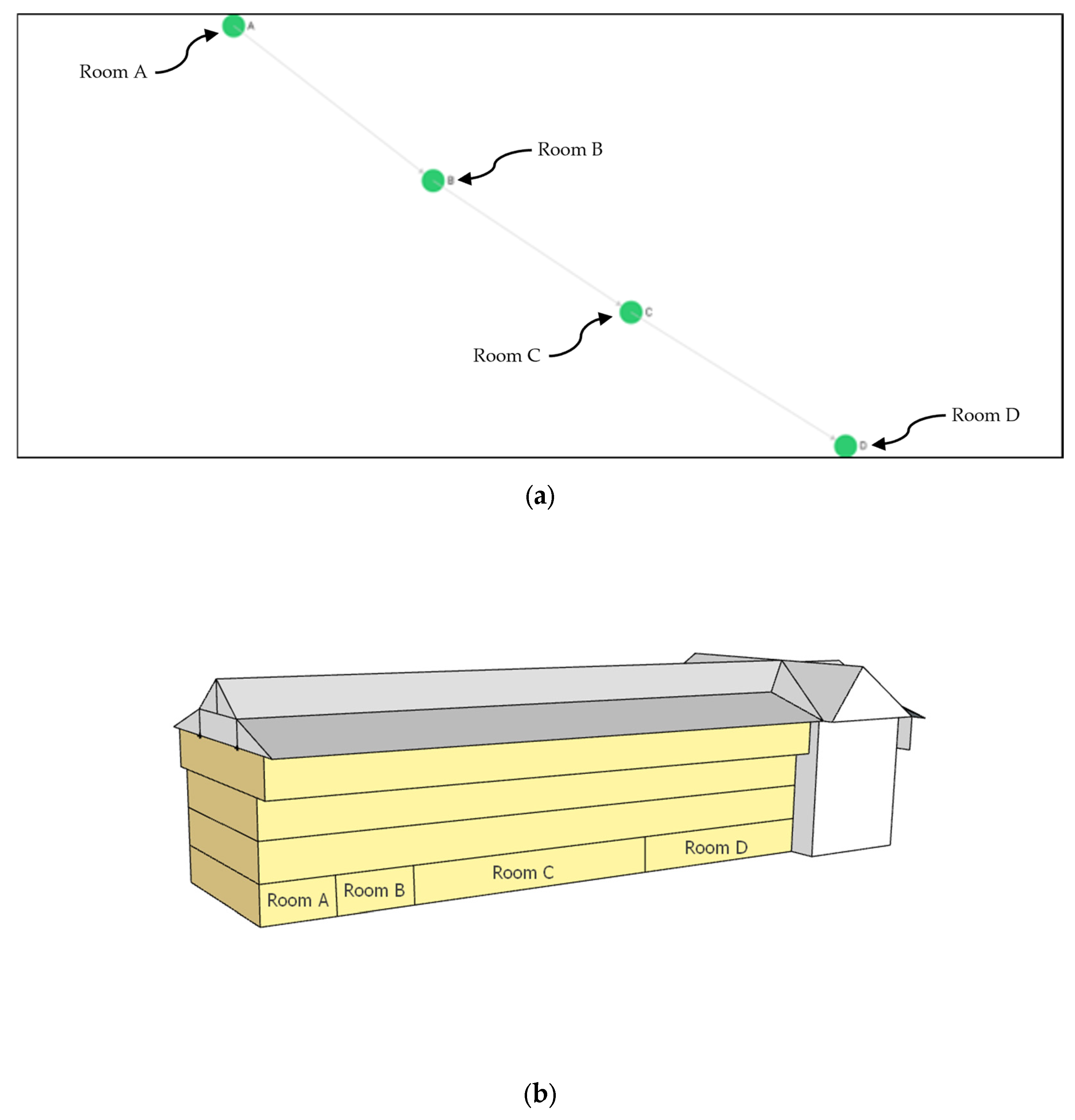
The 3D model illustrating the arrangement of the interior building space in Figure 4 is used to model the interior space shown in Figure 7a. Subsequently, the spatial layer is separated into three main levels, the block, floor, and building space. As the primary entity, the block occupies the initial level. Meanwhile, the building space, which consists of all the rooms, is located at the lowest level. The different levels are connected by several relationships, which are DividedTo, BelongsTo, UpperFloor, and ConnectedTo. Within the graph database, each level will correspond to a distinct database collection, and each collection is related using the aforementioned relationships. DividedTo and BelongsTo are cross-level relationships that describe the containment topology. UpperFloor and ConnectedTo are within-level relationships that describe the adjacency and connectivity topology. The spatial layer in Figure 7a can be illustrated as shown in Figure 7b when it is integrated into the graph database.
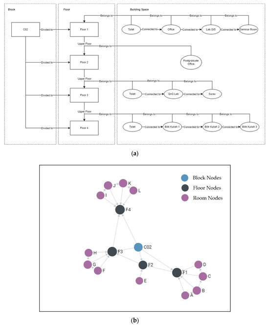
Figure 7.
(a) The complete spatial component of the C02 block; (b) graph view of the C02 block building spaces in the graph database.
However, the building spaces of the building models used in the example in Figure 7 might not accurately reflect the real-world complexity of most building layouts. Typically, buildings have intricate connectivity between spaces. For instance, a floor may contain two rows of rooms that are separated by a central corridor, which might prove to be a more complex and interconnected layout than the example depicted. In this case, the corridors can also be represented as building spaces, similar to other rooms, as they are places where people move around to access rooms and other areas. An example of this scenario is illustrated in Figure 8. Figure 8a shows a simplified representation of building spaces situated on a floor, which consists of multiple rows of rooms that are separated by a corridor. Meanwhile, Figure 8b depicts a graph view of the building layout shown in Figure 8a that has been implemented in the graph database. Similar to the approach used in Figure 7, the building spaces within the same floor are connected using ConnectedTo, which is a topological connectivity relationship that shows the connection and adjacency of corridors and rooms. As denoted in Figure 8, the proposed spatial layer can also accommodate a more complex building layout.
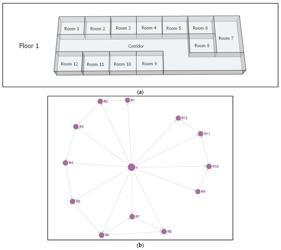
Figure 8.
(a) A simplified representation of multiple rows of rooms; (b) a graph view of multiple rows of building spaces in the graph database.
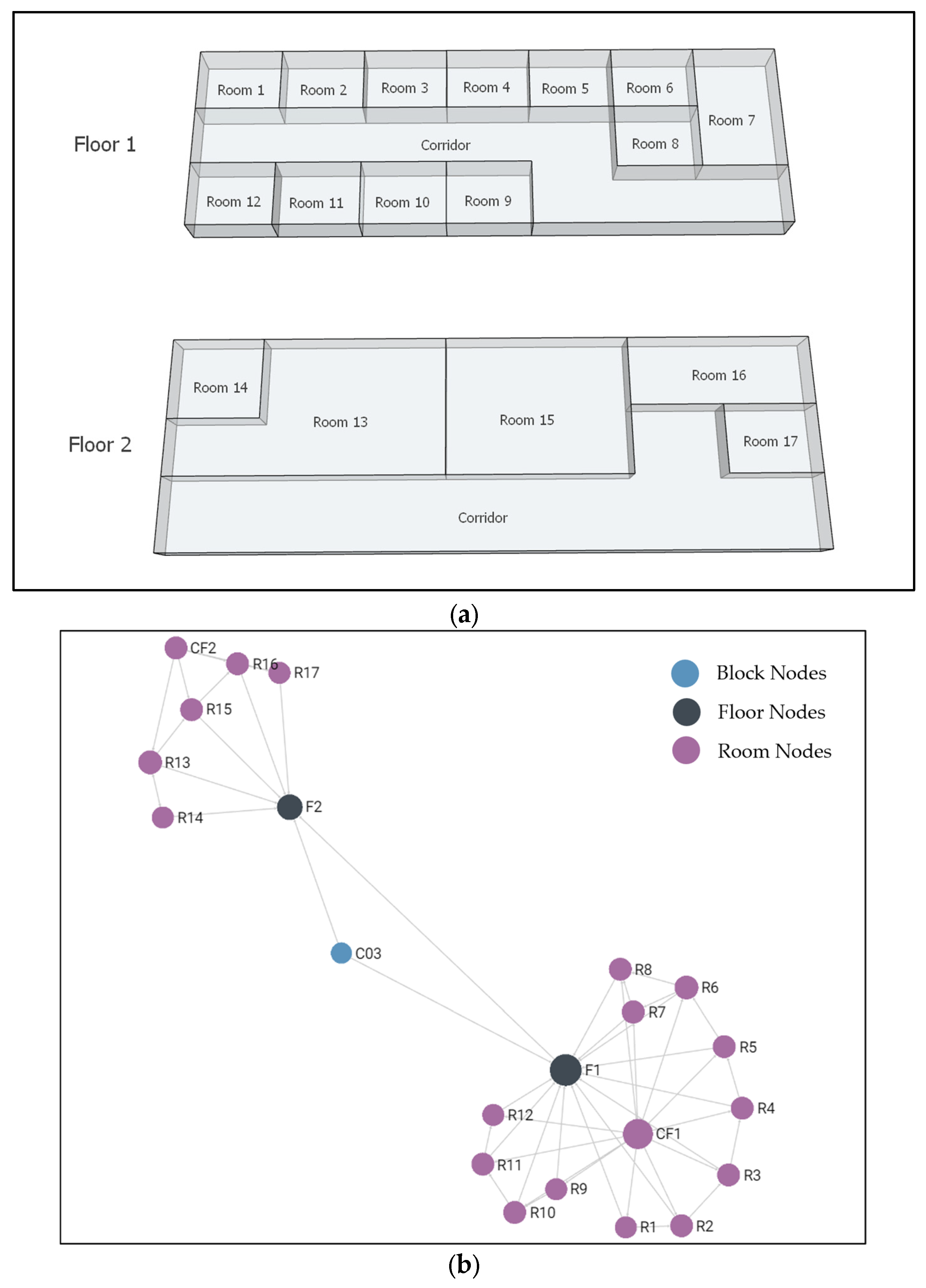
The layouts for multi-story buildings and configurations were further explored, such as when a room is situated within another room. These scenarios add complexity and more accurately reflect real-world situations. Figure 9 illustrates these intricate layouts and their corresponding graph view. The topological containment and connectivity methods presented in this study are designed to accommodate any building layout, regardless of complexity.
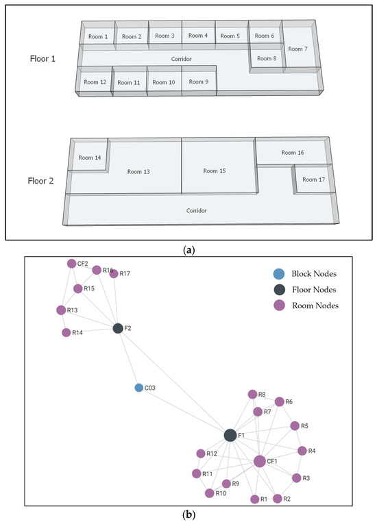
Figure 9.
(a) Simplified representation of building spaces in multi-story buildings; (b) graph view of building spaces in a multi-story building presented in the graph database.
3.2.2. Phase 3: Modelling Temporal Information
Understanding Process Event Data in Asset Management
To formally develop a way to manage the event and the temporal information in asset management, the first step is to describe and understand the process event data in asset management applications. The main form of temporal information in asset management is the historical information in the O&M stages of asset management. Therefore, the management of temporal information is focused primarily on the O&M phase, as it involves various activities to manage the assets, including their operation activity, failure activity, and maintenance activity, as described in Section 3.1. One of the best ways to effectively display historical information is by displaying it chronologically. Through graph modelling, this can be achieved by leveraging a directly-follows graph (DFG).
There are three important information types in process event data in asset management, namely, asset, event, and time information. Where normal process event data, such as purchase-to-pay (P2P) process data would concern event, time information and their case [44], asset information must be included when managing temporal information in asset management. The role of asset information is to relate which assets undergo which events and at what time. In other words, the event information must maintain a relationship with the assets in the spatial layer. As there are many assets to be managed at one time, establishing relationships between asset, event, and time information is complex, primarily because any asset may undergo any activity recurringly at different times [55].
Handling Chronological Flow of Events in Asset Management
Table 1 shows an example of a maintenance record stored chronologically that exists in asset management scenarios. The table consists of the essential asset, activity, and time information with the event ID as additional information to ensure that all records are unique. The table describes the asset and maintenance work that it has undergone, and it can be stored as a graph instance as shown in Figure 10. The sequence of events is stored in the trace column, with the first letter representing the asset and bracketed to distinguish it from other letters. The second letter is the event that the asset underwent, while the subsequent letter is the next maintenance event based on historical records.

Table 1.
Example of historical asset maintenance records.
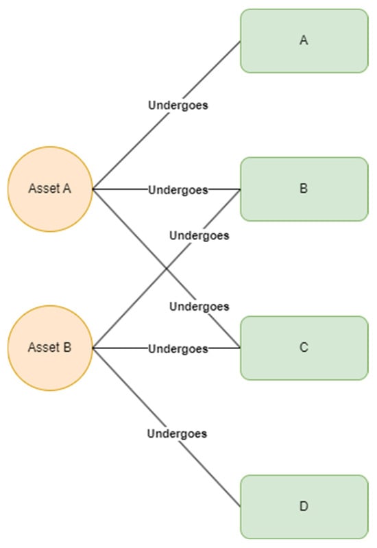
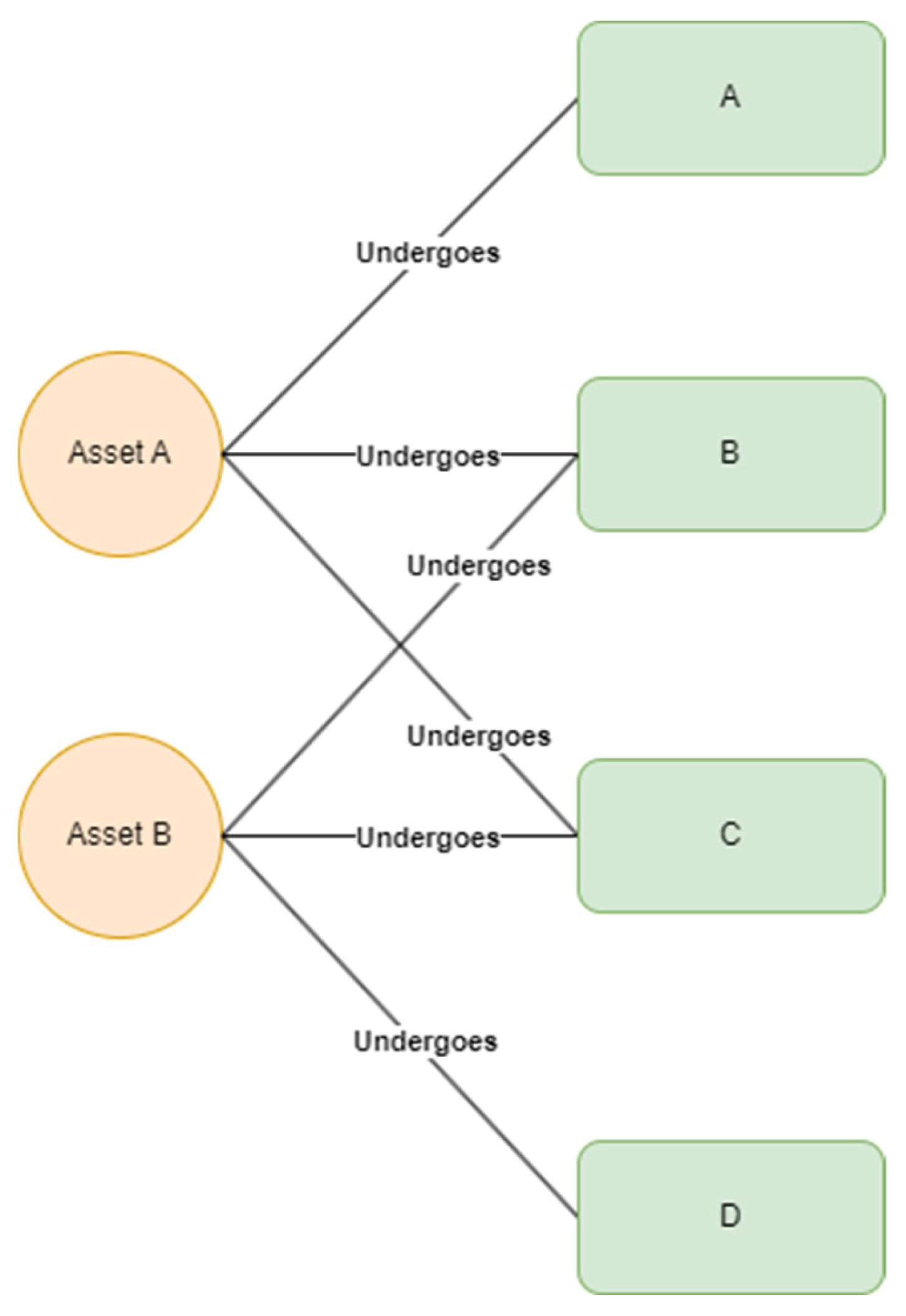
Figure 10.
A graph instance of assets and work.
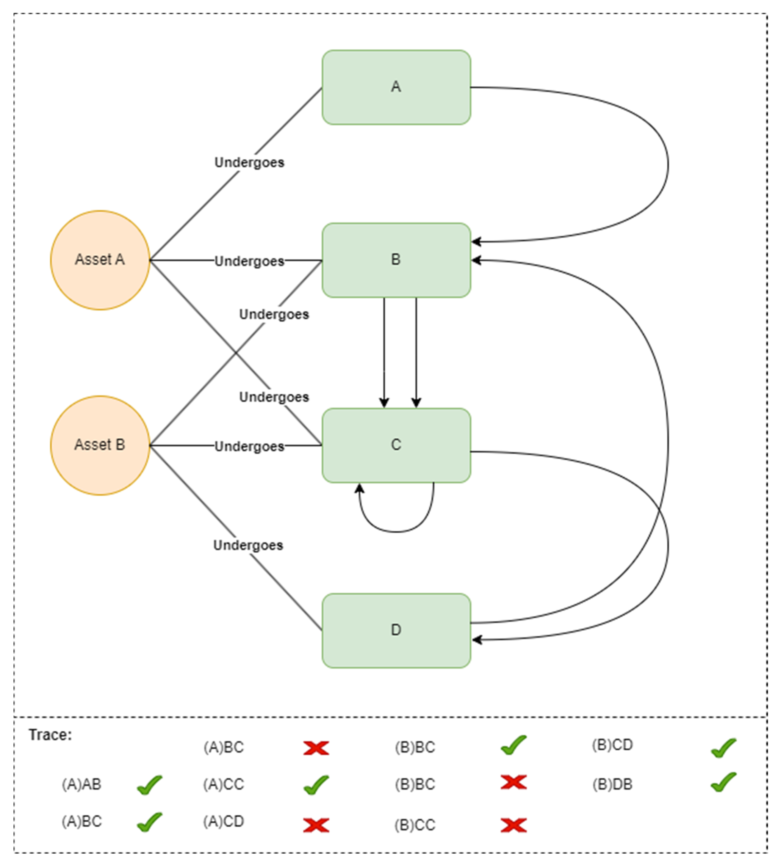
The graph in Figure 10 denotes the assets and work that the asset has undergone. All assets and work are stored in separate nodes, while time is stored inside the event node. The edge relates the assets and work through the undergoes relationship. However, the chronological progression of events shown in Table 1 is obscured when the time information is concealed within the node. A straightforward workaround to circumvent this issue is to flatten the records in Table 1 and introduce a relationship between the events in order to display the event sequence. However, this would introduce a new problem, where a new trace appears that does not exist in the maintenance records. Figure 11 demonstrates the problems when establishing a flattened graph data model to show the sequence of events based on the records in Table 1.

Figure 11.
The appearance of an incorrect trace of events based on a flattened graph model.
As shown in Figure 11, the false traces will contribute to the generation of incorrect queries. This can have a negative impact on the database performance and, consequently, on the asset management decision-making process during the O&M phase.
Research by the authors of [43,44] has demonstrated the problems with a flattened graph model to capture process event information, which is attributed to divergence and convergence issues. Divergence refers to a problem where a single event will lead to multiple possible paths, and convergence is a process where different processes will have a common outcome. In our cases, the problems are primarily divergent as the modelling leads to multiple possible traces that do not exist in reality. This is because the edges between the events that show the trace of the event have no particular differences from other edges. In other words, the edges are not distinctive enough to be differentiated from other traces of the event; hence, they yield wrong and duplicate traces of the event. Asset management is particularly susceptible to the detrimental effects of divergence as the events are usually repeated and the event for an asset happens recurringly. Therefore, obtaining a unique edge is impossible, which in turn creates a false trace.
Furthermore, the querying process in the graph database using the modelling in Figure 11 will be more complex since it involves two-level graph traversals: (1) to query the event that the asset has undergone and (2) to query the sequence of events. A two-level graph traversal query can potentially lead to incorrect query results and be susceptible to obtaining duplicate results. Therefore, modelling the sequence of events requires a more complex and comprehensive way to manage the sequence of events based on a DFG.
A Directly-Follows Graph (DFG) for Managing Chronological Events in Asset Management
This section elaborates on the strategies to mitigate the limitations that have been described in the previous section on how to properly model the flow of events. Therefore, we leveraged the concept of a directly-follows graph (DFG) to describe the sequence of events in process mining applications. A DFG is primarily discussed in the domain of business processes. This study attempts to appropriate and implement the concept of a DFG in asset management to accurately simulate the event flow that occurs repeatedly and recurrently in asset management.
The previous section has described the problem of the multiple false traces that arise due to edges that are not unique and the inefficiency of a flattened event log. The first step to eliminate such a problem is to avoid flattening the event log. This is followed by constructing the chronological sequence of events through a DFG by concentrating solely on the temporal layer while retaining asset information to prevent information loss. This ensures our capability to identify which asset has engaged in which activity. The advantages of focusing the modelling on the temporal layer are twofold. Focusing the modelling on a single layer will eliminate the problem regarding two-level graph traversals, resulting in a straightforward query process that is flexible and guarantees accurate returned queries. The second advantage is the ability to create unique edges by adding more contexts and attributes within the edge relationship that only relate between event entities.
In asset management, where every activity may be completed repetitively, storing each activity as a single node is not the best solution, as it might affect the load operation’s performance inside the database. The insert process will require additional time and additional database storage, thus producing a database with poor performance. To circumvent this issue, we implement node aggregation by grouping all nodes with common activity characteristics into one single node; hence, all activity nodes are unique. For example, all the assets may go through construction activity nine times; instead of inserting the construction activity as nine different nodes, we can aggregate all nine nodes into one single construction node. Consequently, it will reduce the storage size of the database. To show the sequence of events, the node activity will connect to the succeeding activity through directly-follows (DF) relationships.
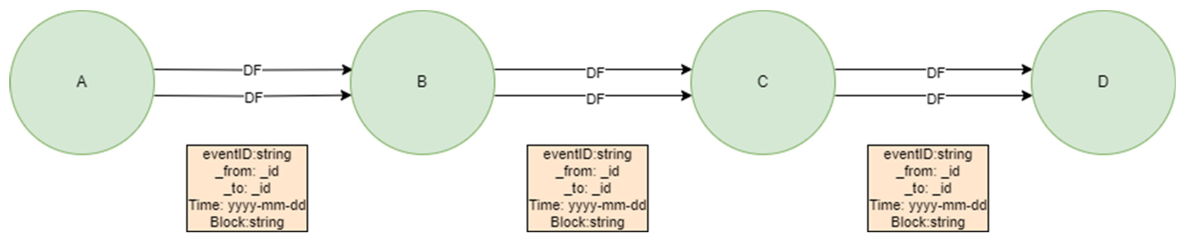
However, aggregating all common activities into a single node will not solve the problems with edges that are not unique. The only way to solve this issue is by manipulating the edge. This can be completed by connecting the edge between event nodes multiple times through DF relations. To impose uniqueness on each edge, event IDs are stored inside the edge relationship; hence, no two edges will be the same even though they relate to the same set of activities. The asset and time information will also be stored within the edge to provide more information when the DF relation is queried. Connecting the event node multiple times between the same event node will essentially form this graph into a multigraph. Therefore, from this point forward, this method will be described as the Aggregated Directly-Follows Multigraph (ADFM) and is defined in Definition 4. The concept of the ADFM is shown in Figure 12 below. In Figure 12, the letter in each node refers to the event as shown in Table 1.
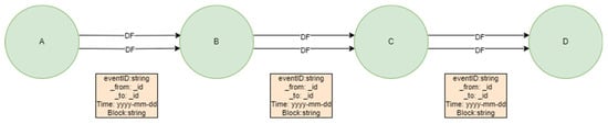
Figure 12.
Aggregated Directly-Follows Multigraph (ADFM).
Definition 4 (Aggregated Directly-Follows Multigraph).
The Aggregated Directly-Follows Multigraph (ADFM) is a graph G = (N, E), where
- N is a set of nodes and E is a set of directed edges.
- N = { | A= (a1, a2, …, an)}, ai is an activity recorded in at least one trace, t of the event log, where each ai is a unique activity node aggregated from all instances of the same activity.
- E={(ai, aj)|ai, aj∈N}, where each edge (ai, aj) represents a directed “directly-follows” relation from ai to aj with possible edge repetition from ai and aj.
The ADFM focuses on the event or temporal layer based on Figure 12, where the nodes only represent the event information. The edge only relates between event nodes to represent the DF relationship to show which event succeeds an event. It also contains important information that adds richer context to the DF relationship, including the event ID, the temporal information, and the asset information. The event ID is included for two purposes: (1) to guarantee the uniqueness of each record and (2) as filterable attributes during the querying process. The temporal information based on the figure refers to the date when the preceding event occurred, which is stored in the edge rather than in the event node to guarantee the uniqueness of the aggregated event nodes. Meanwhile, the asset information is stored within the edge to indicate which asset undergoes the event. The asset node from Figure 11 was omitted to facilitate the construction of a single-level graph traversal that emphasises only the temporal layer to query the sequence of events.
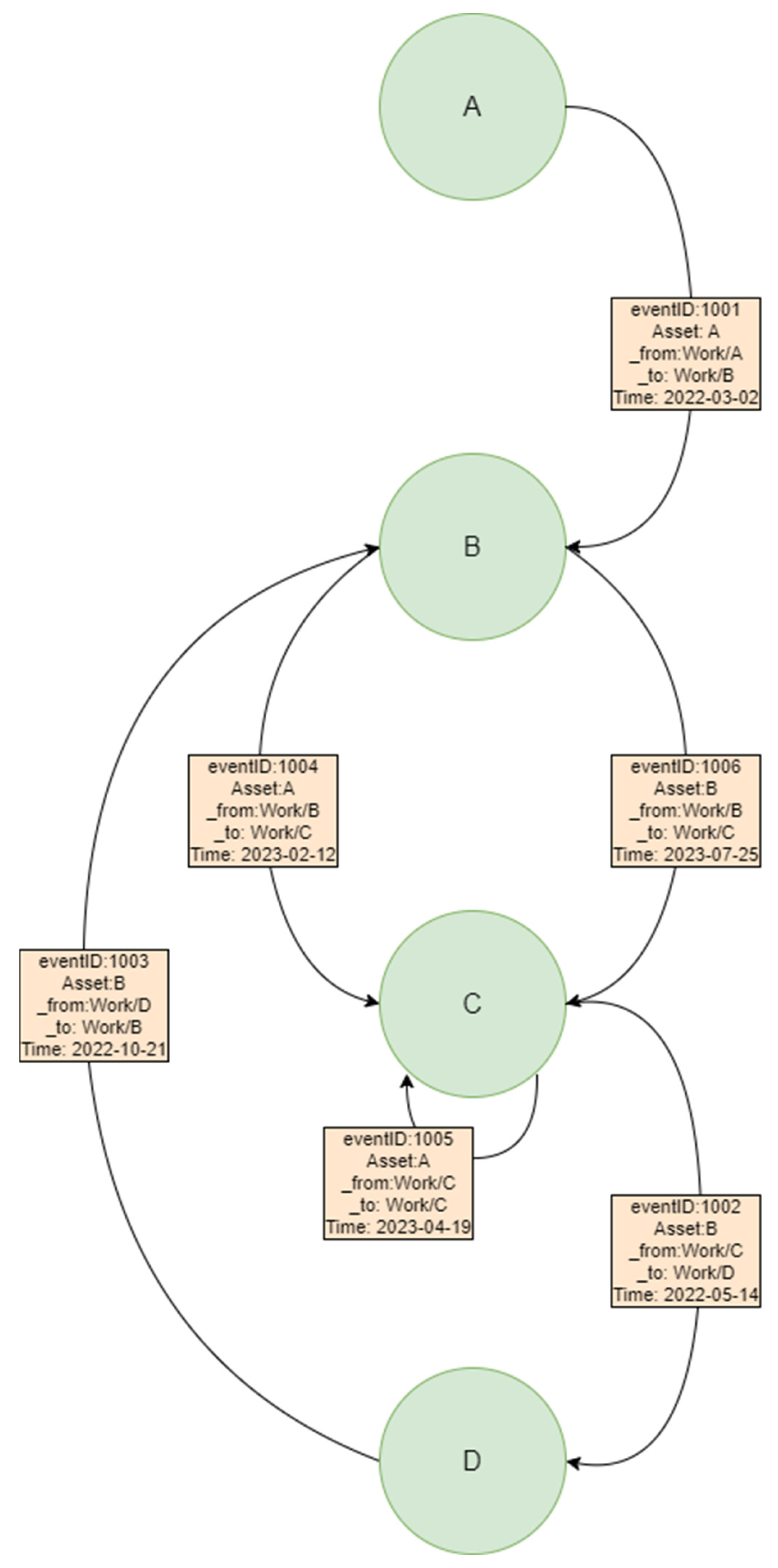
Finally, the description of the ADFM serves as a fundamental for constructing a complete process event log in Table 1. Figure 13 shows the modelling of process event log based on ADFM. The letter in each node in Figure 13 refers to the event as shown in Table 1. From Figure 13, we can see that all edges are unique with the appearance of the event ID, the trace of events, and the timestamp. The multigraph notion in the DF relationship exists between events B and C, where it is connected multiple times, involving different assets while also ensuring that the edges are distinct.

Figure 13.
Modelling of process event log based on the ADFM.
3.2.3. Phase 4: Integrating the Spatial and Temporal Model
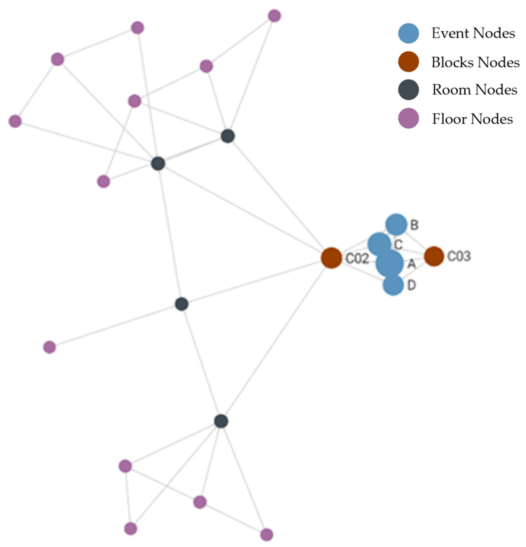
The approach to model spatial and temporal data, through the arrangement of building spaces and the management of the chronological flow of event data, has been adequately delineated. We can further outline the appropriate method to integrate the spatial and temporal data to construct a comprehensive spatio-temporal model for asset management purposes. The integration of both layers is illustrated in Figure 14, where blue nodes depict event nodes, red nodes indicate block nodes, black nodes indicate room nodes, and purple nodes indicate floor nodes. The spatial component at any level (see Figure 9) is subjected to any activities in the O&M phases. In order to establish the connection between information in the spatial and temporal layers, it is necessary to define a relationship between the two types of information in each layer. Therefore, we retain the undergoes relationship presented in Figure 10, describing which asset undergoes which event. Using this relationship, we can identify which asset has undergone which event as well as other queries, such as aggregation queries of event and asset information.
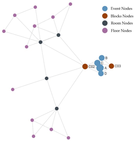
Figure 14.
The resultant integration of spatial and temporal layers in ArangoDB.
4. Evaluation of the Data Model
This section illustrates the data model’s query capability through the execution of a query pertaining to the asset management maintenance phase. The query is divided into two categories, which are the spatial query and the temporal query. It should be noted that the data model is implemented in the ArangoDB graph database. Therefore, the query is based on the ArangoDB Query Language (AQL).
4.1. Spatial Query
The formulisation of Queries 1 and 2 is based on a use case on asset maintenance, where in some cases, the inspection and maintenance of a building are conducted by external contractors hired specifically to address specific issues. These individuals may not be familiar with the building’s layout and, therefore, require guidance to locate the rooms where inspection or maintenance is needed. Therefore, it is necessary to provide ways to guide these individuals in navigating a building across multiple floors and traversing various rooms on each floor. Query 1 identifies a room by specifying the block and floor where the room is located. Query 2 reveals the adjacency between rooms on the same floor.
- Query 1: Containment Query
The objective of this query is to locate a room that is the lowest-level entity of the spatial model. This query involves the containment relationship and can be made by filtering the ID or the name of the room by modifying the @BuildingSpace parameter inside the query. The parameter @BuildingSpace is a bind parameter in the AQL that allows users to insert any filterable attributes without modifying the query. The following query will return the ID and name of the room and the floor and building where the room is located.
| Query 1: Finding where a room is located | |
| 1 | FOR v,e,p |
| 2 | IN 2..2 |
| 3 | OUTBOUND @BuildingSpace BelongsTo, INBOUND DividedTo |
| 4 | RETURN {RoomID: p.vertices [0]._key, RoomName: p.vertices [0].Name, Floor: p.vertices [1]._key, Block: p.vertices [2]._key} |
- Query 2: Adjacency Query
The purpose of this query is to determine which rooms are connected to a certain room. In other words, it returns the room that shares the same boundary wall with a specific room. This query involves the adjacency relationship and utilises the bind parameter to filter which room the user desires to be queried.
| Query 2: Finding adjacency of building spaces | |
| 1 | FOR v,e,p |
| 2 | IN 1..1 |
| 3 | ANY @BuildingSpace ConnectedTo |
| 4 | RETURN {RoomID:v._key, RoomName:v.Name} |
Alternatively, a user who wishes to ascertain the complete extent of the building space connectivity within a floor may alter the query to retrieve the graph view of the query. It will visually represent the whole length of the building space connection. This involves the user specifying a large upper bound number for the path length as they may not know the precise quantity of rooms situated on a certain floor. However, the query will still return the correct number of rooms situated on a floor.
| Query 2 (Alternative): Finding connectivity of building spaces | |
| 1 | FOR v,e,p |
| 2 | IN 1..100 |
| 3 | ANY @BuildingSpace ConnectedTo |
| 4 | RETURN p |
4.2. Temporal Query
The temporal query for the evaluation of this data model is separated into three queries, corresponding to three use cases involving asset maintenance practices. Query 1 is based on first use cases, which involve asset managers that are required to ascertain which asset has undergone which event and the status of the event. This process is essential to enable the efficient scheduling of maintenance operations, ensuring that each asset receives the necessary attention based on its activity history and condition. Furthermore, understanding the event history of assets is vital for effective cost management. By keeping track of events, asset managers can analyse the total cost for maintenance, replacements, or failures and make informed financial decisions.
Query 2 plays a part in risk management, which is a crucial task in asset management. Identifying the frequency of an asset experiencing specific events, such as failures or accidents, allows asset managers to assess risks and implement preventive measures. Asset managers can accomplish this by finding the amount of time an asset has gone through a specific event. Asset managers can identify patterns and potential vulnerabilities by determining the number of operational failures or downtime experienced by an asset.
Finally, for Query 3, it is imperative to understand the sequence and timing of events to allow better coordination and optimisation of operations. Asset managers can guarantee the timely and efficient execution of all asset management activities, consequently minimising downtime and enhancing overall operational efficiency. They need to identify the sequence of events to improve the efficiency of the asset operation. The formulation and strategy for each query are explained in detail below.
- Query 1: Which asset has undergone specific maintenance?
The first query is finding the asset that has undergone a specific maintenance event. This query is completed over the undergoes relationship, which is the spatio-temporal layer of the data model, since it relates to the asset (i.e., spatial elements) and events (i.e., temporal elements). Asset managers may require information regarding the maintenance status and completion time to ensure that no asset has been neglected during the maintenance process and to schedule subsequent maintenance activities.
| Query 1: Finding the asset that has undergone a specific event | |
| 1 | FOR c IN Work |
| 2 | FILTER c.Name == @Work |
| 3 | FOR v, e, p IN 1..1 OUTBOUND c Undergoes |
| 4 | return {eventID:e.eventID, Block:e.Block, Work:c.Name, Time:e.Time} |
- Query 2: Aggregation of event
The result from Query 1 may not clearly demonstrate the frequency of maintenance work. Therefore, it will aggregate the amount of time and frequency of a maintenance event undergone by the asset. The filterable attributes are the name of the asset and the type of maintenance work. This query is also completed over the undergoes relationship.
| Query 2: Finding the amount of time an asset has gone through a specific event | |
| 1 | FOR c in Blocks |
| 2 | FILTER c.BlockName == @Blocks |
| 3 | FOR v, e, p IN 1..1 OUTBOUND c Undergoes |
| 4 | FILTER v.Name == @Work |
| 5 | COLLECT BlockName = c.BlockName INTO Grouped |
| 6 | RETURN {Block: BlockName, Frequency: LENGTH(Grouped)} |
- Query 3: Querying the directly-follows relation.
This query will determine the sequence of events by querying the DirectlyFollow relationship.
| Query 3: Finding the sequence of events | |
| 1 | FOR c IN Work |
| 2 | FOR v, e, p IN 1..1 OUTBOUND c DirectlyFollow |
| 3 | FILTER e.eventID == @eventID |
| 4 | RETURN {eventID:e.eventID, Block:e.Block, Work:c.Name, Time:e.Time, NextEvent:v.Name} |
The query will return the event that directly follows an event by filtering the event ID. The asset and work can also be filtered as an alternative to filtering solely by the event ID.
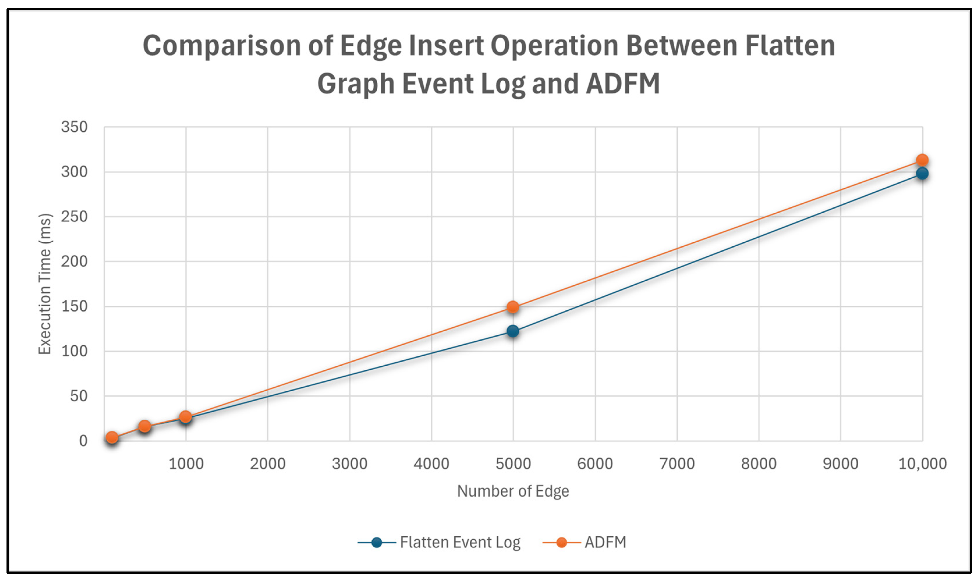
4.3. Comparison of the Insert Operation between Flattened Graph Event Log and the ADFM
One of the differences between a flattened graph event log and the ADFM is how the DF relationship is developed. The DF relationship in the ADFM uses more attributes to add more information to the edge relationship, as an effort to reduce the graph traversals from two-level to single-level graph traversals. Therefore, the insert operation for the edge might be influenced by the amount of information that is available within the DF relationship.
Figure 15 visualises the result of the insert operation of the edge between the two approaches. The operation was completed on ArangoDB using the AQL function, enabling the user to obtain the execution time. The numbers of edges tested were 100, 500, 1000, 5000, and 10,000 for both approaches. As seen from the figure, the execution time for both approaches increases linearly, with the ADFM possessing a longer execution time for the insert operation across all numbers of edges. The key difference between both approaches is the edge attributes within the edge, and this occurrence is afflicted by the number of edge attributes within the ADFM that are larger than the flattened event log. As a comparison, the edges of the flattened graph event log and the ADFM consist of three and five attributes, respectively. The type of edge attributes for both approaches is shown in Table 2. This signifies a trade-off for the ADFM, which offers a more straightforward and accurate query, although a longer execution time is observed for the insert operation.
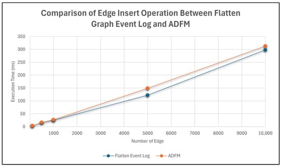
Figure 15.
Comparison of the edge insert operation between the flattened event log and the ADFM.
Table 2.
Edge attributes for both approaches.
5. Discussion
This paper introduces a spatio-temporal data model for asset management applications, which consists of two main layers, which are the spatial and temporal layers. The spatial layer focuses on modelling the component of interior building space arrangements. The initial building space arrangements are acquired from the visualisation of a 3D city model, which is then modelled using graph notation, where each component is treated as a node, while the relationship between components is denoted using edges. The modelling of the interior building space arrangement is facilitated by an edge relationship that shows the containment and connectivity relationship of elements in the interior building space to allow a graph view of the building space arrangement, as shown in Figure 16. The graph illustrated in Figure 16a shows the full length of the building connection of a building space located on a floor, where the building space is identified by its alphabetical identification. Meanwhile, Figure 16b illustrates the room arrangement of the first floor for C02 block, from which the graph view of the building connection shown in Figure 16a is derived. This method enables the implementation of indoor navigation through the utilisation of NoSQL graph databases, which have been demonstrated to offer clearer representations via graph visualisation. Consequently, the modelling of the interior building space using graphs offers an alternative to high-LoD 3D city models. Illustrating the containment and connectivity relationship also serves as key topological information for the management of 3D objects within spatial databases to allow more complex spatial queries [56].
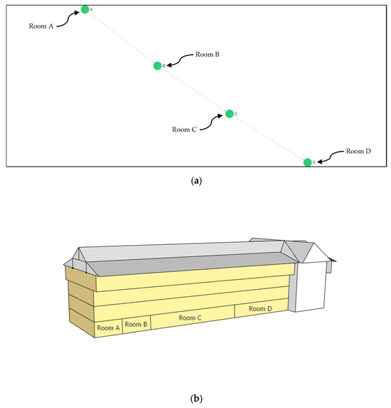
Figure 16.
(a) A graph view of building space connection for the first floor of C02 block; (b) the room arrangement for the first floor of C02 Block.
The ADFM was introduced in the temporal layer as a graph model to show the chronological sequence of repetitive events stored in a graph database. This model leverages the notion of the Directly-Follows Multigraph (DFM) introduced by the author of [57] as an object-centric process mining approach, which has proven to provide a more realistic view of process event data. The main difference introduced by this paper is implementing it in a graph database alongside elucidating the factors and strategies that must be considered when implementing it in a graph database. The main characteristic of this model is the aggregation of event nodes and the separation of temporal information from nodes, which, alternatively, are stored within the directly-follows edge relation. This approach produced a graph data model, where both the node and edge are unique, in an effort to solve the issue of false traces, when querying the sequence of events from a flattened event log. The difference between the ADFM and a flattened event log in Figure 11 is shown in Table 3.
Table 3.
Difference between a flattened event log and the ADFM.
Asset management is a dynamic activity with ever-changing events that will be undergone by assets. The proposed ADFM model facilitates understanding the sequence of activities and extracting information through queries to conduct analysis that can enhance O&M phases in asset management. With many new activities that an asset will undergo on a daily basis, it is imperative that the model can accommodate changes and updates of activities. The proposed model is designed to be adaptable to allow new events to be added and linked to the respective assets undergoing the activity. This is essential to ensure that the data remains current and reflective of the asset’s latest activities.
The problem when modelling the event log (see Figure 11) is that the false trace arises from the edges that are not unique and the two-level graph traversal queries to relate the asset and their DF relation. Table 4 shows the difference in query complexities between the ADFM and a flattened event log to query the DF relation. The flattened event log consists of a two-level graph traversal query, which in turn necessitates a more complex query strategy. As a consequence of the edge lacking essential information, which includes the asset and temporal information, the query process will return all the records that are connected with the filtered attributes, as no specific information can be filtered to differentiate the edge. Consequently, false traces and duplicate records are produced for this reason. Unlike the ADFM, which consists of a single-level graph traversal query, the query strategy to gather the sequence of events is more straightforward. Furthermore, as all the important information is stored within the edge, all filterable attributes can be filtered in one single query. A correct result from the query can thus be guaranteed as a result of multiple edges that are unique.
Table 4.
The difference in the query strategies between a flattened event log and the ADFM.
6. Conclusions
In this paper, we introduced a spatio-temporal graph data model for the application of asset management, concentrating on the management of the bi-dimensional information within the graph database. The variety of information in asset management has been identified and adapted to our data model, which consists of spatial and temporal layers. In the spatial layer, we introduced a graph-based building space management that separates a building component into three levels, which are the block, floor, and building space. The elements in each level are connected to each other through cross-level relationships or within-level relationships. These two types of relationships allow containment and adjacency relationships to be established between relevant components to allow spatial queries pertaining to containment and connectivity information of 3D model elements.
In the temporal layer, the main objective is to model the chronological flow of events in asset management using graph notation. The primary concern is resolving the issue with repetitive events in asset management, which may result in inaccurate event traces when event logs are modelled as flattened graph data models due to divergence issues, which are prevalent in the process mining domain. Therefore, we introduce the Aggregated Directly-Follows Multigraph (ADFM) to counter the issue of repetitive events in any business process application. Our model involves aggregating all repetitive events into one single node, creating a unique set of event nodes. To show the chronological flow of the event log, multiple edges are connected between relevant event nodes through a directly-follows relationship. The multiple edges between the same set of nodes are differentiated by inserting event ID information within the edge to enforce the integrity and uniqueness of each edge to ensure that the correct flow of events is acquired when queried.
There is a limitation concerning the proposed ADFM. The limitation concerns the insert operation, where the execution time for loading edge information in the ADFM is longer when compared to the flattened graph event log. This increased execution time is due to the edge attributes that exist within the ADFM that are larger than the flattened event log. However, it is a necessary drawback to provide a data model with a straightforward query and accurate query results. This balance between the insert operation and query accuracy is essential in information management applications for developing a robust and effective data model that meets the needs of sophisticated data management and analysis tasks.
Furthermore, the integration of the spatial and temporal layers constitutes the main component of the spatio-temporal data model, allowing spatio-temporal queries to ascertain which asset has undergone which event. Although such a query is temporal, it requires the integration of both layers to produce an efficient model that enables flexible queries to retain query accuracy. It is hoped that the findings of this paper provide necessary insights for further research on the management of 3D city model information using NoSQL databases, particularly graph databases. In the context of asset management, our findings offer key information for researchers and asset managers to manage historical records of activity, particularly in the O&M phase of asset management. This paper also provides a way to manage and manipulate temporal information using graph modelling to support an active and data-driven asset maintenance strategy through Predictive Maintenance (PdM).
Author Contributions
Conceptualization, Muhammad Syafiq and Suhaibah Azri; formal analysis, Muhammad Syafiq; methodology, Muhammad Syafiq and Suhaibah Azri; supervision, Suhaibah Azri; Validation, Muhammad Syafiq and Suhaibah Azri; visualization, Muhammad Syafiq; writing—original draft, Muhammad Syafiq; writing—review and editing, Suhaibah Azri and Uznir Ujang. All authors have read and agreed to the published version of the manuscript.
Funding
This work was supported by the Ministry of Higher Education through the Fundamental Research Grant Scheme (FRGS/1/2022/WAB07/UTM/02/3).
Data Availability Statement
The raw data supporting the conclusions of this article will be made available by the authors upon request.
Acknowledgments
The highest appreciation is offered to UTMNexus scholarship for sponsoring the study of the first author.
Conflicts of Interest
The authors declare no conflicts of interest.
References
- Demirdöğen, G.; Işık, Z.; Arayici, Y. BIM-Based Big Data Analytic System for Healthcare Facility Management. J. Build. Eng. 2023, 64, 105713. [Google Scholar] [CrossRef]
- Zonta, T.; da Costa, C.A.; da Rosa Righi, R.; de Lima, M.J.; da Trindade, E.S.; Li, G.P. Predictive Maintenance in the Industry 4.0: A Systematic Literature Review. Comput. Ind. Eng. 2020, 150, 106889. [Google Scholar] [CrossRef]
- Munir, M.; Kiviniemi, A.; Finnegan, S.; Jones, S.W. BIM Business Value for Asset Owners through Effective Asset Information Management. Facilities 2020, 38, 181–200. [Google Scholar] [CrossRef]
- McMahon, P.; Zhang, T.; Dwight, R. Requirements for Big Data Adoption for Railway Asset Management. IEEE Access 2020, 8, 15543–15564. [Google Scholar] [CrossRef]
- Lafioune, N.; Desmarest, A.; Poirier, É.A.; St-Jacques, M. Digital Transformation in Municipalities for the Planning, Delivery, Use and Management of Infrastructure Assets: Strategic and Organizational Framework. Sustain. Futur. 2023, 6, 100119. [Google Scholar] [CrossRef]
- Chang, J.Y.; Garcia, J.M.; Xie, X.; Moretti, N.; Parlikad, A. Information Quality for Effective Asset Management: A Literature Review. IFAC-PapersOnLine 2022, 55, 235–240. [Google Scholar] [CrossRef]
- Moretti, N.; Xie, X.; Garcia, J.M.; Chang, J.; Parlikad, A.K. Built Environment Data Modelling: A Review of Current Approaches and Standards Supporting Asset Management. IFAC-PapersOnLine 2022, 55, 229–234. [Google Scholar] [CrossRef]
- Moretti, N.; Xie, X.; Merino Garcia, J.; Chang, J.; Kumar Parlikad, A. Federated Data Modeling for Built Environment Digital Twins. J. Comput. Civ. Eng. 2023, 37, 04023013. [Google Scholar] [CrossRef]
- Polenghi, A.; Roda, I.; Macchi, M.; Pozzetti, A. Information as a Key Dimension to Develop Industrial Asset Management in Manufacturing. J. Qual. Maint. Eng. 2022, 28, 567–583. [Google Scholar] [CrossRef]
- Chen, W.; Chen, K.; Cheng, J.C.P.; Wang, Q.; Gan, V.J.L. BIM-Based Framework for Automatic Scheduling of Facility Maintenance Work Orders. Autom. Constr. 2018, 91, 15–30. [Google Scholar] [CrossRef]
- Koukias, A.; Nadoveza, D.; Kiritsis, D. Semantic Data Model for Operation and Maintenance of the Engineering Asset. In IFIP Advances in Information and Communication Technology; Springer: Berlin/Heidelberg, Germany, 2013; pp. 49–55. ISBN 9783642403606. [Google Scholar]
- Halfaway, M.R.; Vanier, D.J.; Froese, T.M. Standard Data Models for Interoperability of Municipal Infrastructure Asset Management Systems. Can. J. Civ. Eng. 2006, 33, 1459–1469. [Google Scholar] [CrossRef]
- Marquez, A.C.; Fernandez, J.F.G.; Fernández, P.M.G.; Lopez, A.G. Maintenance Management through Intelligent Asset Management Platforms (IAMP). Emerging Factors, Key Impact Areas and Data Models. Energies 2020, 13, 3762. [Google Scholar] [CrossRef]
- Martínez García, D.; Lee, J.; Keck, J.; Yang, P.; Guzzetta, R. Spatiotemporal and Deterioration Assessment of Water Main Failures. AWWA Water Sci. 2019, 1, e1159. [Google Scholar] [CrossRef]
- Ganesan, S.G.; García, D.M.; Lee, J.; Keck, J.; Yang, P. A Spatio-Temporal Water Mains Integrity Management Program for California. World Environ. Water Resour. Congr. 2017, 489, 523–533. [Google Scholar]
- Iglesias, V.; Braswell, A.E.; Rossi, M.W.; Joseph, M.B.; McShane, C.; Cattau, M.; Koontz, M.J.; McGlinchy, J.; Nagy, R.C.; Balch, J.; et al. Risky Development: Increasing Exposure to Natural Hazards in the United States. Earth’s Futur. 2021, 9, e2020EF001795. [Google Scholar] [CrossRef]
- Pittore, M.; Wieland, M.; Fleming, K. Perspectives on Global Dynamic Exposure Modelling for Geo-Risk Assessment. Nat. Hazards 2017, 86, 7–30. [Google Scholar] [CrossRef]
- Mestav Sarica, G.; Zhu, T.; Pan, T.C. Spatio-Temporal Dynamics in Seismic Exposure of Asian Megacities: Past, Present and Future. Environ. Res. Lett. 2020, 15, 094092. [Google Scholar] [CrossRef]
- Cammerer, H.; Thieken, A.H.; Verburg, P.H. Spatio-Temporal Dynamics in the Flood Exposure Due to Land Use Changes in the Alpine Lech Valley in Tyrol (Austria). Nat. Hazards 2013, 68, 1243–1270. [Google Scholar] [CrossRef]
- Fuchs, S.; Keiler, M.; Zischg, A. A Spatiotemporal Multi-Hazard Exposure Assessment Based on Property Data. Nat. Hazards Earth Syst. Sci. 2015, 15, 2127–2142. [Google Scholar] [CrossRef]
- Biljecki, F.; Lim, J.; Crawford, J.; Moraru, D.; Tauscher, H.; Konde, A.; Adouane, K.; Lawrence, S.; Janssen, P.; Stouffs, R. Extending CityGML for IFC-Sourced 3D City Models. Autom. Constr. 2021, 121, 103440. [Google Scholar] [CrossRef]
- Greyling, B.T.; Jooste, W. The Application of Business Process Mining to Improving a Physical Asset Management Process: A Case Study. S. Afr. J. Ind. Eng. 2017, 28, 120–132. [Google Scholar] [CrossRef]
- Brous, P.; Janssen, M.; Herder, P. Internet of Things Adoption for Reconfiguring Decision-Making Processes in Asset Management. Bus. Process Manag. J. 2019, 25, 495–511. [Google Scholar] [CrossRef]
- Wakiru, J.M.; Pintelon, L.; Muchiri, P.; Chemweno, P. A Comparative Analysis of Maintenance Strategies and Data Application in Asset Performance Management for Both Developed and Developing Countries. Int. J. Qual. Reliab. Manag. 2022, 39, 961–983. [Google Scholar] [CrossRef]
- Khoury, G.; Figueiredo, M. Improved Decision-Making, Safety and Reliability with Visual Asset Performance Management. In Proceedings of the Abu Dhabi International Petroleum Exhibition and Conference, Abu Dhabi, UAE, 9–12 November 2020. [Google Scholar] [CrossRef]
- Jalali, A. Graph-Based Process Mining. In Process Mining Workshop; Springer International Publishing: Berlin/Heidelberg, Germany, 2020; pp. 273–285. [Google Scholar]
- Jalali, A. Object Type Clustering Using Markov Directly-Follow Multigraph in Object-Centric Process Mining. IEEE Access 2022, 10, 126569–126579. [Google Scholar] [CrossRef]
- Leemans, S.J.J.; Poppe, E.; Wynn, M.T. Directly Follows-Based Process Mining: Exploration & a Case Study. In Proceedings of the 2019 International Conference on Process Mining (ICPM), Aachen, Germany, 24–26 June 2019; pp. 25–32. [Google Scholar] [CrossRef]
- Singh, S.; Shehab, E.; Higgins, N.; Fowler, K.; Reynolds, D.; Erkoyuncu, J.A.; Gadd, P. Data Management for Developing Digital Twin Ontology Model. Proc. Inst. Mech. Eng. Part B J. Eng. Manuf. 2021, 235, 2323–2337. [Google Scholar] [CrossRef]
- Yang, X.; Koehl, M.; Grussenmeyer, P.; Macher, H. Complementarity of Historic Building Information Modelling and Geographic Information Systems. In Proceedings of the XXIII ISPRS Congress, Prague, Czech Republic, 12–19 July 2016. [Google Scholar] [CrossRef]
- Yang, X.; Grussenmeyer, P.; Koehl, M.; Macher, H.; Murtiyoso, A.; Landes, T. Review of Built Heritage Modelling: Integration of HBIM and Other Information Techniques. J. Cult. Herit. 2020, 46, 350–360. [Google Scholar] [CrossRef]
- Caldera, S.; Mostafa, S.; Desha, C.; Mohamed, S. Exploring the Role of Digital Infrastructure Asset Management Tools for Resilient Linear Infrastructure Outcomes in Cities and Towns: A Systematic Literature Review. Sustainability 2021, 13, 11965. [Google Scholar] [CrossRef]
- Song, Y.; Wang, X.; Tan, Y.; Wu, P.; Sutrisna, M.; Cheng, J.C.P.; Hampson, K. Trends and Opportunities of BIM-GIS Integration in the Architecture, Engineering and Construction Industry: A Review from a Spatio-Temporal Statistical Perspective. ISPRS Int. J. Geo-Inf. 2017, 6, 397. [Google Scholar] [CrossRef]
- Garramone, M.; Moretti, N.; Scaioni, M.; Ellul, C.; Re Cecconi, F.; Dejaco, M.C. BIM and GIS Integration For Infrastructure Asset Management: A Bibliometric Analysis. ISPRS Ann. Photogramm. Remote Sens. Spat. Inf. Sci. 2020, 6, 77–84. [Google Scholar] [CrossRef]
- Xue, F.; Wu, L.; Lu, W. Semantic Enrichment of Building and City Information Models: A Ten-Year Review. Adv. Eng. Inform. 2021, 47, 101245. [Google Scholar] [CrossRef]
- Vishnu, E.; Sameer, S. OGC CityGML 3D City Models Enriched with Utility Infrastructures for Developing Countries. J. Indian Soc. Remote Sens. 2021, 49, 813–826. [Google Scholar] [CrossRef]
- Nasir, A.A.M.; Azri, S.; Ujang, U. Managing 3D Asset Management Using CityGML Concept. J. Inf. Syst. Technol. Manag. 2022, 7, 139–147. [Google Scholar] [CrossRef]
- Lei, B.; Stouffs, R.; Biljecki, F. Assessing and Benchmarking 3D City Models. Int. J. Geogr. Inf. Sci. 2023, 37, 788–809. [Google Scholar] [CrossRef]
- Kolbe, T.H. Representing and Exchanging 3D City Models with CityGML. In 3D Geo-Information Sciences; Lee, J., Zlatanova, S., Eds.; Lecture Notes in Geoinformation and Cartography; Springer: Berlin/Heidelberg, Germany, 2009; pp. 15–31. [Google Scholar] [CrossRef]
- Gröger, G.; Plümer, L. CityGML—Interoperable Semantic 3D City Models. ISPRS J. Photogramm. Remote Sens. 2012, 71, 12–33. [Google Scholar] [CrossRef]
- Nasir, A.A.M.; Azri, S.; Ujang, U.; Choon, T.L. Managing Indoor Movable Assets in 3D Using CityGML for Smart City Applications. Int. Arch. Photogramm. Remote Sens. Spat. Inf. Sci. 2022, XLVIII, 19–21. [Google Scholar] [CrossRef]
- Zhou, Y.W.; Hu, Z.Z.; Lin, J.R.; Zhang, J.P. A Review on 3D Spatial Data Analytics for Building Information Models. Arch. Comput. Methods Eng. 2020, 27, 1449–1463. [Google Scholar] [CrossRef]
- Chapela-Campa, D.; Dumas, M.; Mucientes, M.; Lama, M. Efficient Edge Filtering of Directly-Follows Graphs for Process Mining. Inf. Sci. 2022, 610, 830–846. [Google Scholar] [CrossRef]
- Van Der Aalst, W.M.P. A Practitioner’s Guide to Process Mining: Limitations of the Directly-Follows Graph. Procedia Comput. Sci. 2019, 164, 321–328. [Google Scholar] [CrossRef]
- Esser, S. Using Graph Data Structures for Event Logs. Zenodo 2019. [Google Scholar] [CrossRef]
- Augusto, A.; Dumas, M.; La Rosa, M.; Leemans, S.J.J.; vanden Broucke, S.K.L.M. Optimization Framework for DFG-Based Automated Process Discovery Approaches. Softw. Syst. Model. 2021, 20, 1245–1270. [Google Scholar] [CrossRef]
- Li, L.; Dai, F. Transformation and Visualization of BPMN Models to Petri Nets. IOP Conf. Ser. Earth Environ. Sci. 2018, 186, 012047. [Google Scholar] [CrossRef]
- Peterson, J.L. Petri Nets. ACM Comput. Surv. 1977, 9, 223–252. [Google Scholar] [CrossRef]
- Augusto, A.; Conforti, R.; Dumas, M.; La Rosa, M.; Maggi, F.M.; Marrella, A.; Mecella, M.; Soo, A. Automated Discovery of Process Models from Event Logs: Review and Benchmark. IEEE Trans. Knowl. Data Eng. 2019, 31, 686–705. [Google Scholar] [CrossRef]
- Esser, S.; Fahland, D. Storing and Querying Multi-Dimensional Process Event Logs Using Graph Databases. In Business Process Management Workshops: BPM 2019 International Workshops; Springer International Publishing: Vienna, Austria, 2019; Volume 17, ISBN 9783030374525. [Google Scholar]
- Debrouvier, A.; Parodi, E.; Perazzo, M.; Soliani, V.; Vaisman, A. A Model and Query Language for Temporal Graph Databases. VLDB J. 2021, 30, 825–858. [Google Scholar] [CrossRef]
- Al-Kasasbeh, M.; Abudayyeh, O.; Liu, H. An Integrated Decision Support System for Building Asset Management Based on BIM and Work Breakdown Structure. J. Build. Eng. 2021, 34, 101959. [Google Scholar] [CrossRef]
- Biljecki, F.; Kumar, K.; Nagel, C. CityGML Application Domain Extension (ADE): Overview of Developments. Open Geospat. Data Softw. Stand. 2018, 3, 13. [Google Scholar] [CrossRef]
- Ledoux, H.; Arroyo Ohori, K.; Kumar, K.; Dukai, B.; Labetski, A.; Vitalis, S. CityJSON: A Compact and Easy-to-Use Encoding of the CityGML Data Model. Open Geospat. Data Softw. Stand. 2019, 4, 4. [Google Scholar] [CrossRef]
- Syafiq, M.; Azri, S.; Ujang, U. Modelling Reoccurrence of Events in an Event-Based Graph Database for Asset Management. In Proceedings of the 2023 4th International Conference on Artificial Intelligence and Data Sciences (AiDAS), IPOH, Malaysia, 6–7 September 2023; pp. 102–108. [Google Scholar] [CrossRef]
- Salleh, S.; Ujang, U.; Azri, S. Topology Models and Rules: A 3D Spatial Database Approach. Int. Arch. Photogramm. Remote Sens. Spat. Inf. Sci. 2023, XLVIII-1/W, 117–122. [Google Scholar] [CrossRef]
- van der Aalst, W.M.P. Object-Centric Process Mining: Dealing with Divergence and Convergence in Event Data. In Software Engineering and Formal Methods. SEFM 2019; Ölveczky, P., Salaün, G., Eds.; Lecture Notes in Computer Science; Springer: Cham, Switzerland, 2019; Volume 11724. [Google Scholar] [CrossRef]


Disclaimer/Publisher’s Note: The statements, opinions and data contained in all publications are solely those of the individual author(s) and contributor(s) and not of MDPI and/or the editor(s). MDPI and/or the editor(s) disclaim responsibility for any injury to people or property resulting from any ideas, methods, instructions or products referred to in the content. |
© 2024 by the authors. Published by MDPI on behalf of the International Society for Photogrammetry and Remote Sensing. Licensee MDPI, Basel, Switzerland. This article is an open access article distributed under the terms and conditions of the Creative Commons Attribution (CC BY) license (https://creativecommons.org/licenses/by/4.0/).