Beyond the Road: A Regional Perspective on Traffic Congestion in Metro Atlanta

Abstract

Traffic congestion not only affects traffic flow but also influences public perception of congested regions. While analyzing congestion at the road section level can help identify engineering solutions, it often fails to reveal broader spatial patterns and trends at the regional or macro scale unless summarized effectively. This study aims to address these challenges by focusing on regional-scale traffic congestion amounts measured by distanceTime metrics. A 12–month dataset, sampled every 10 min, was analyzed to identify spatial patterns, temporal trends, regional variations, and predictive models in the Metro Atlanta area. The results show that congestion is the most severe and increasing at key urban corridors like Brookhaven–Sandy Springs, the downtown connector, Druid Hills–Decatur, and Johns Creek–Cumming, aligning with recent urban developments. Cities such as Alpharetta, Dunwoody, Brookhaven, Austell, Stone Mountain, East Point, Lake City, Morrow, Fairburn, and Jonesboro show high increasing trends in congestion. Predictive modeling with the long short-term memory (LSTM) method shows promising results for short-term forecasts, though variability in data requires further optimization for certain cities. This research is significant because it demonstrates that congestion amounts measured by distanceTime metrics can be used for assessing regional characteristics broadly at a metropolitan city scale. The findings and methodologies identified in this research might support urban and transportation planning efforts in metropolitan planning organizations, such as the Atlanta Regional Commission, by identifying congestion amounts and trends at both the regional and road scales.

1. Introduction

Traffic congestion is a pervasive issue that not only impacts the efficiency of transportation systems but also shapes public perception and quality of life in urban areas [1,2,3,4,5]. As urban populations continue to grow, understanding the dynamics of traffic congestion becomes increasingly vital [6]. While localized analyses at the road section level can yield valuable engineering insights, they often fail to capture the broader spatial and temporal dynamics that characterize congestion across entire regions [7,8,9,10]. This limitation hinders our understanding of how congestion patterns evolve and interact over time, ultimately affecting urban planning and policymaking. To address these challenges, this study shifts focus from micro-level assessments to a macro, regional-level examination of traffic congestion.

Analyzing traffic congestion is an important, mandatory part of urban planning in U.S.A. metropolitan areas. For example, the Atlanta Regional Commission (ARC), a metropolitan planning organization (MPO), analyzes traffic congestion as a part of the congestion management process in their Metropolitan Transportation Plan (MTP) [11]. The Delaware Valley Regional Planning Commission, an MPO of the Greater Philadelphia region, also shows a comprehensive congestion management process [12]. Indeed, the congestion management process is mandated by federal legislation under the Surface Transportation Act (23 CFR Parts 450.322 and 500.109) for urbanized areas with populations exceeding 200,000, referred to as Transportation Management Areas [13]. These regulations require that the congestion management process be integrated continuously into the metropolitan planning process.

Effective congestion management relies heavily on the collection of high-quality data over extended periods [14], which is often hindered by the constraints of limited resources [15]. At a regional scale, traffic congestion has been measured using multiple methods. One method is to use delay time [10,16,17]. As an application example, INRIX, Inc. (Kirkland, WA, USA), a company specializing in traffic analytics, reports traffic delay time and its economic cost in a region every year [18]. INRIX uses cellphones, vehicle tracking, and Global Positioning System (GPS) data to estimate travel time and speeds. Congestion is noted when speed drops below a certain rate against free-flow speed. The INRIX delay time data are proprietary and have limitations regarding user-customized access. Another method is to use navigation maps’ application programming interface (API). For example, many research articles were published using Google Maps Platform APIs [19] to calculate multiple origin–destination routes to estimate regional traffic congestion (e.g., [20,21,22,23]). The API method is highly flexible and effective when applied to specific routes. However, it has limitations in accurately representing regional-scale congestion levels unless the samples are selected in a valid, representative, and reliable manner. Another method is to use online traffic status maps and calculate the traffic congestion amount with a three-dimensional (3D) space–time cube. For instance, Seong et al. [24] introduced the “distanceTime” metric to quantify congestion amounts in six major metropolitan areas across the U.S.A., and Kim et al. [25] utilized this metric to analyze congestion on the interstate highway in downtown Atlanta, Georgia. The online traffic map approach could be a viable alternative when funding is limited. By leveraging real-time data, this approach can enhance the overall effectiveness of congestion management efforts while making efficient use of available resources.

As implied in the ARC’s Metropolitan Transportation Plan [11], congestion management primarily targets major congestion corridors, which play a vital role in addressing broader traffic challenges across metropolitan areas. While this focus is essential for understanding and mitigating congestion on larger roadways, it is equally important to consider the levels of congestion in smaller subregions, including local cities and counties. These areas often experience unique traffic patterns and issues that can significantly impact local mobility and quality of life. Unfortunately, current methodologies frequently fail to provide satisfactory solutions tailored to the specific needs of individual local governments. As a result, local authorities may lack the tools and data necessary to effectively address congestion in their jurisdictions. This oversight can lead to a disconnect between regional strategies and local realities, ultimately hindering the effectiveness of congestion management efforts. By broadening the focus to include localized congestion data and solutions, local government might create a more comprehensive approach that not only alleviates traffic in major corridors but also supports the unique requirements of smaller communities.

In this context, this study aims to (1) identify spatial and temporal patterns, (2) analyze temporal trends, (3) summarize regional variations, and (4) model and predict trends. In this research, we used Google traffic congestion maps to identify congestion amounts [26]. The online traffic map approach is highly scalable and facilitates the effective summarization of congestion amounts by subregions [24,26]. Using the distanceTime traffic congestion amounts proposed by Seong et al. [24], this research analyzes spatial patterns and temporal trends using geographic information systems (GISs), time series analysis methods, and long short-term memory (LSTM) modeling and prediction techniques. This study provides a robust methodological framework for regional traffic congestion analysis that may support urban planners and policymakers with essential insights for making informed decisions. This, in turn, might enhance transportation efficiency and improve the overall livability of urban environments.

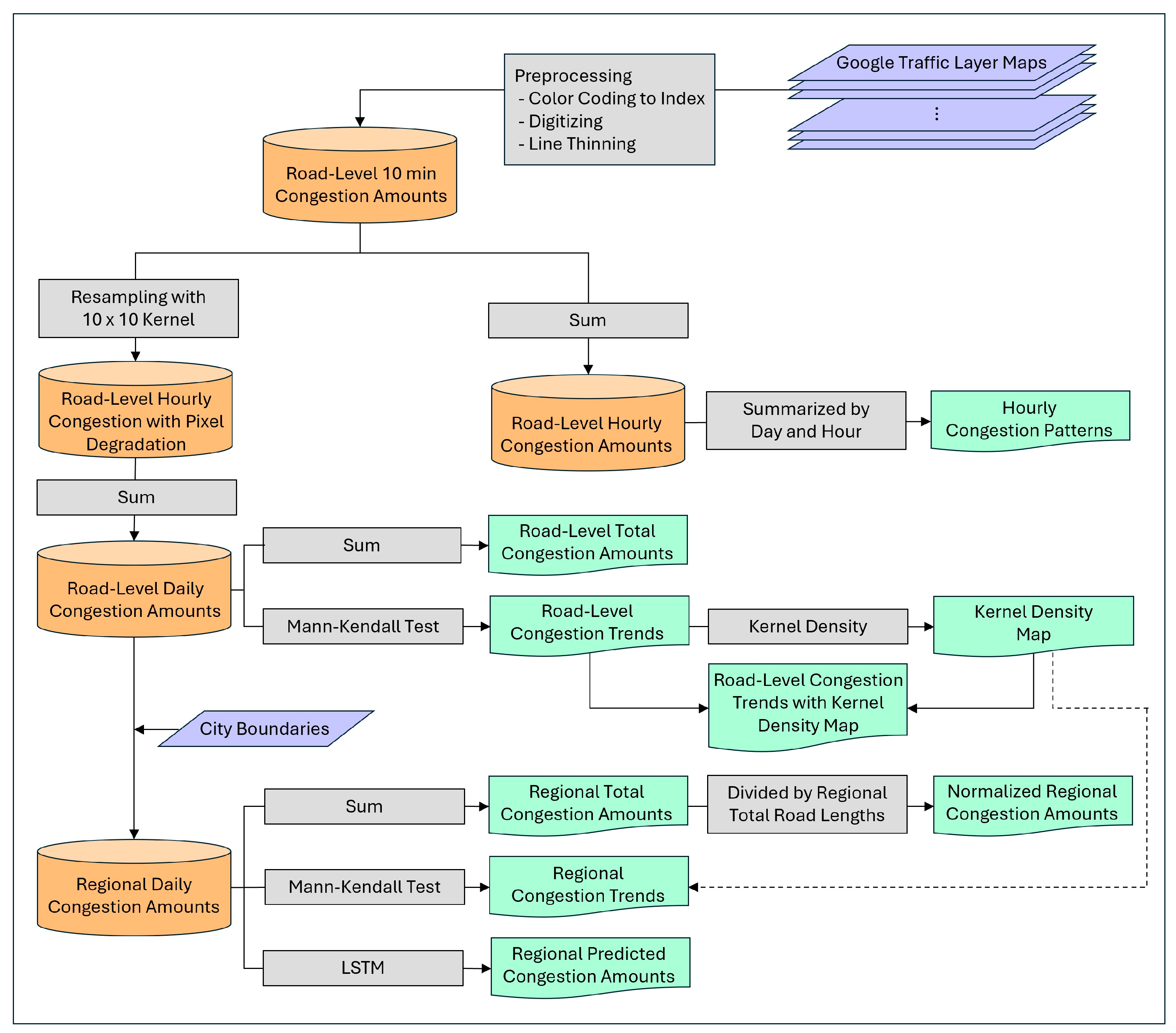
2. Materials and Methods

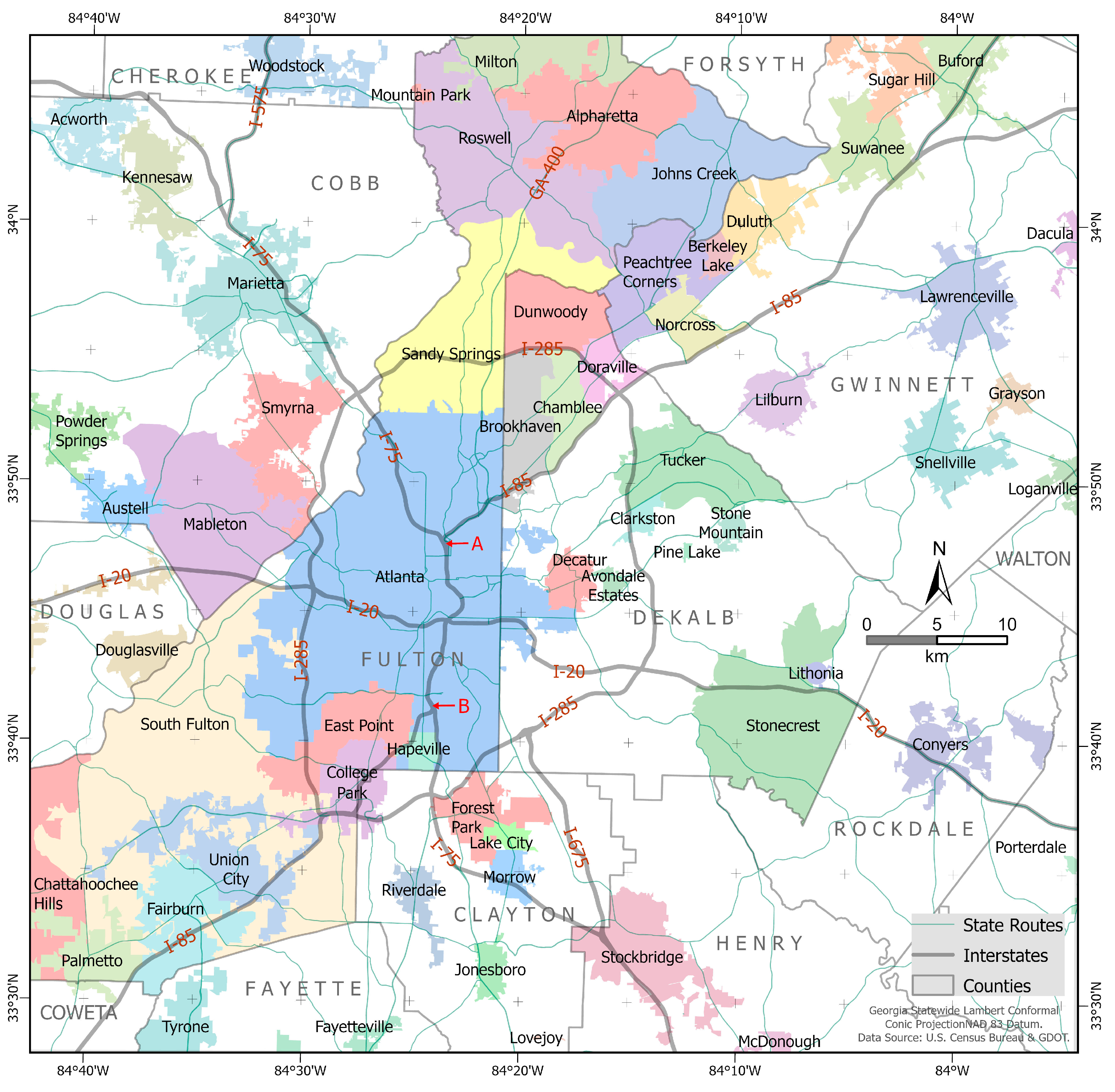
2.1. Study Area and Data

Figure 1 shows the study area, the Metro Atlanta area in Georgia, U.S.A., with various cities shaded in distinct colors, including the cities of Atlanta, Sandy Springs, Roswell, Johns Creek, Marietta, Decatur, Union City, Morrow, Forest Park, and Stonecrest, among others. Metro Atlanta’s interstate highways play a key role in moving people, goods, and emergency vehicles within the region and across the southeast, and about half of all vehicle miles traveled in the metro area are on these highways [11]. Major interstates, such as I–20, I–75, and I–85, pass through the urban center. Although I–285 helps divert through traffic as the only freeway loop, the radial road network, resembling a wheel-and-spoke pattern, contributes to significant traffic congestion. This is especially noticeable at major interstate intersections, such as the downtown corridor, where I–75 and I–85 converge in the city of Atlanta, as well as at key intersections along I–285. According to the Atlanta Regional Commission [11], about 1.8 million more residents are expected to call the Atlanta region home by 2050, and, consequently, the region calls for over 600 lane miles of additional capacity along the surface arterial network. In this context, the ARC MTP’s major roadway projects planned by 2050 include sections of I–285 north of I–20, I–20 on I–285, GA–400, I–85 north of I–285, I–75 south of I–285, and multiple arterial roads mainly located in the eastern half of the area, particularly outside I–285. Given that the population density in the top half of the study area is significantly higher than in the bottom half, traffic congestion in Metro Atlanta is expected to remain a persistent issue in the coming decades.

Figure 2 summarizes the workflow that was performed in this research. First of all, raw traffic congestion data were collected every 10 min using the Google Maps API and the Google Traffic Layer for the study area, which covered a total of 5045 km of roads, from 1 April 2022 to 31 March 2023. The Google Traffic Layer represents congestion severity with colors as follows: green for no delays, orange for medium traffic, red for traffic delays, and dark red for heavy delays. These color-coded pixels were indexed by numerical values of 0, 1, 2, and 4, corresponding to green, orange, red, and dark red, respectively. The 10 min samples were further aggregated spatially to make approximately 253 m pixels using the maximum value in each 10 × 10 kernel window and then temporally aggregated to produce hourly and daily layers by averaging pixel values.

2.2. Spatial and Temporal Patterns

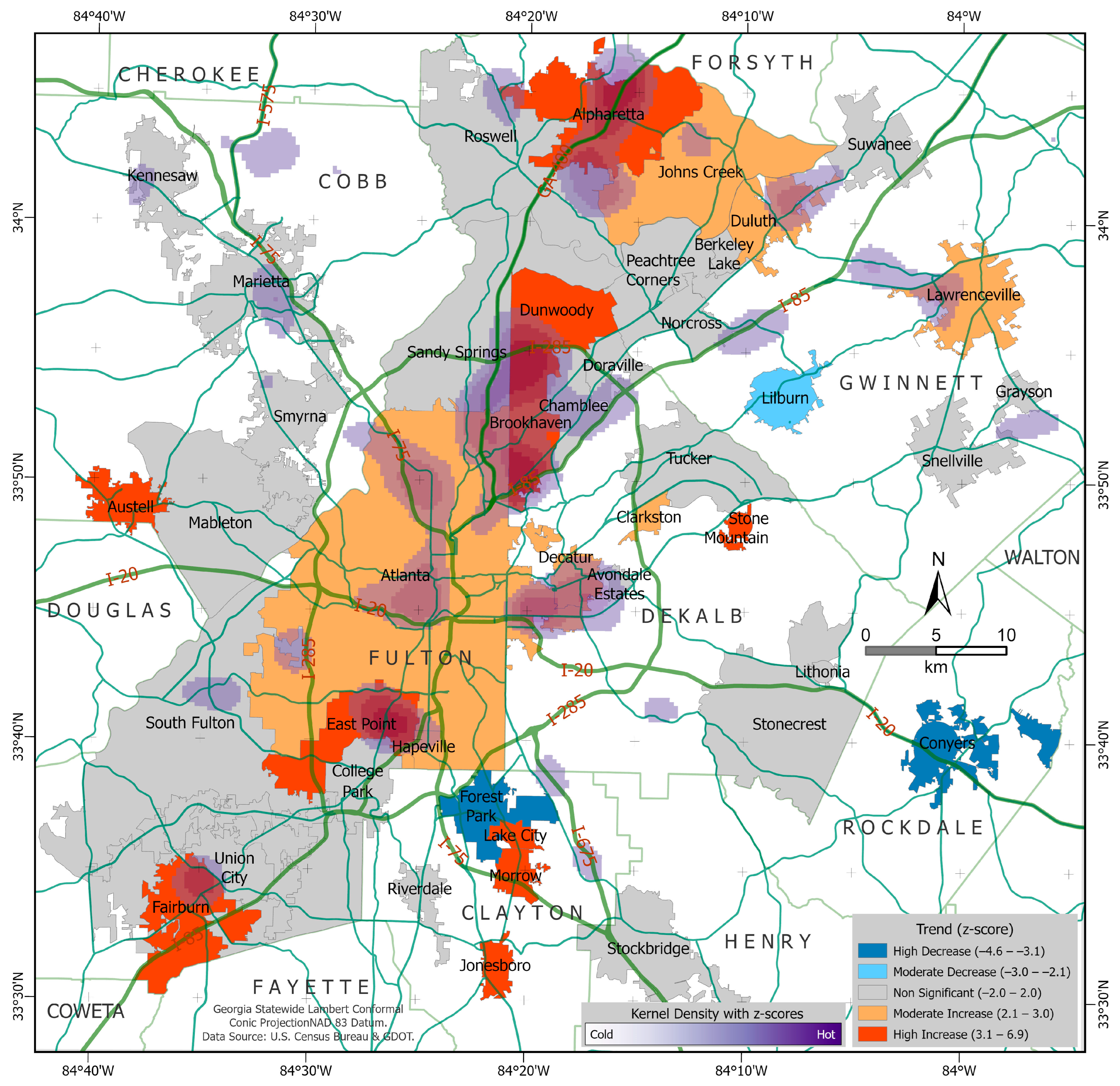
The following procedure was used to calculate the traffic congestion amount, x, from n sample images for a sampling period, p, with a pixel distance, d: (1) the congestion index was scaled from values of 0, 1, 2, or 4 to 0, 0.25, 0.5, or 1.0 by dividing by 4; (2) the average of the n samples was calculated for each pixel to obtain the average temporal congestion for that pixel; (3) the pixel distance, d, was multiplied by the average temporal congestion to calculate the congestion distance for the sampling period, p; and (4) the sampling period, p, was multiplied by the congestion distance to obtain the distanceTime congestion amount for the sampling period, p. Similarly to how a battery’s capacity is measured by combining two properties, such as watt-hours, the distanceTime unit merges spatial and temporal properties to represent congestion amounts in a specific area over a given period, which helps overcome the limitations of measuring congestion by only using the time or spatial domain individually [24]. In sum, when congestion levels are coded with 0, 1, 2, or 4, the traffic congestion amount, x, with pixel digital numbers, DNs, can be calculated as follows:

x = Σ (DNs)/(4 × n) × d × p

(1)

In the case of this study, a congestion map was developed by calculating the congestion amount in each pixel. First, all 10 min sample layers were added pixel-wise, and the pixel-wise sum was divided by 4. The number was further divided by 6 to obtain the hourly congestion amount, by 144 to obtain the daily congestion amount, and by 52,560 to obtain the annual congestion amount. Regarding the pixel distance, the diameter of an imaginary circle of which area is equivalent to the areal size of a pixel was used, considering all possible directions of a road in a pixel. The resulting pixel distance (d) was 285.374 m (i.e., d = 2 r, where r = sqrt(pixelArea/π). Congestion distance was calculated by multiplying 285.374 m and the average temporal congestion amount. Then, the sampling period was multiplied to obtain the distanceTime metrics. The distanceTime metrics were used in various formats, such as meterYear, mileHour, mileDay, and mileYear, to name a few.

To examine regional hot and cold spots, kernel densities were calculated. The kernel density operation calculates the density of features in a neighborhood around those features, and, optionally, feature attribute values can be used. The congestion amount in each pixel was used to create a kernel density map layer. Kernel density (ρ) was calculated using a quartic kernel [27,28] as follows:

$$\rho ={\displaystyle \frac{1}{r^2}}\sum _{i=1}^n\left[{\displaystyle \frac{3}{\pi }}·w_i{\left(1-{\left({\displaystyle \frac{d_i}{r}}\right)}^2\right)}^2\right]$$

(2)

where r is the search radius, n is the number of incidents within the search radius, w is the attribute value, and d is the distance between the kernel center and an incident inside the search radius. The density, ρ, is multiplied by the number of incidents or the sum of the attribute field. In this research, a 350 m output pixel size was used, and the default search radius that was generated by ArcGIS Pro [27] was used with the Silverman’s Rule of Thumb [28] that is robust enough for spatial outliers.

2.3. Trend Analysis

To analyze the temporal trend, the Mann–Kendall test (MKT) was conducted in a Python environment using daily congestion amounts. The MKT evaluates trends in a time series dataset with the null hypothesis (H₀), stating that there is no trend, and the alternative hypothesis (H_A), indicating either an increasing or decreasing trend [29,30]. The original MKT was applied to the daily total congestion amounts. The seasonal Mann–Kendall test was not applied because the dataset spans only one year. Furthermore, covariates such as population growth and major congestion-inducing events were not included due to the relatively short data collection period and the challenges in quantifying significant congestion-inducing events.

In a time series, x₁, …, x_n, the MKT statistic, S, is calculated as follows:

$$S={\sum }_{i=1}^{n-1}{\sum }_{j=i+1}^{n}sgn(x_j-x_i)$$

(3)

where the sgn() is −1, 0, or 1 if (x_j − x_i) is less than, equal to, or larger than 0, respectively. Then, the variance of S is calculated as follows:

$$Var\left(S\right)={\displaystyle \frac{1}{18}}\left[n\left(n-1\right)\left(2n+5\right)-\sum _p^g{t}_p(t_p-1)(2t_p+5)\right]$$

(4)

where g is the number of tied groups, and t_p is the number of observations in the pth group. Finally, the Mann–Kendall test statistic, z, is calculated as follows:

$$z=\left\{\begin{array}{cc}(S-1)/\sqrt{Var\left(S\right)},& if S>0\\ 0,& if S=0\\ (S+1)/\sqrt{Var\left(S\right)},& if S<0\end{array}\right.$$

(5)

If there is no monotonic trend (i.e., the null hypothesis), then for a time series with more than 10 elements, z has a standard normal distribution with a mean and a standard deviation of 0 and 1, respectively. A significantly large positive z value indicates an increasing trend, while a significantly small negative z value indicates a decreasing trend.

2.4. Regional Analysis

To examine regional differences, daily congestion data were organized by city using the GIS zonal overlay operation using the U.S. Census Bureau’s 2023 Incorporated Places dataset [31,32]. City boundaries were used as subregions because counties were only partially included in the study area. Furthermore, cities are key partners of the Atlanta Regional Commission, which is responsible for metropolitan transportation planning. As illustrated in Figure 1, there are forty-five cities in the study area, excluding partially included cities. Among them, two cities (Mountain Park and Pine Lake) did not overlap with the sampled roads and were therefore excluded from the analysis. To assess regional variations, the total congestion in each city was calculated by accumulating all congestion amounts. After identifying temporal trends in individual cities using the Mann–Kendall test, prediction models were developed with a time series dataset for each city using the LSTM method.

LSTM is a recurrent neural network (RNN) model designed to overcome the problem of long-term dependencies inherent in traditional RNNs [33,34]. RNNs are primarily used for processing sequential data by predicting outputs based on the hidden state from previous time steps [35]. However, as the number of steps increases, earlier information tends to be lost, making RNNs effective only for short sequences [33]. To address this limitation, LSTM uses input gates, forget gates, and output gates in the memory cell of the hidden layer. These gates decide which information to remember and which to forget, enabling the model to store necessary information and make predictions. As a result, LSTM is particularly effective in tasks such as time series forecasting and natural language processing, where understanding the patterns and relationships of past information is crucial. For example, Kim [25] predicted traffic congestion patterns on the downtown connector in Atlanta. Xu [36] successfully predicted morning traffic flow in Beijing, China, using LSTM. Mojtaba et al. [37] also used LSTM with daily traffic data in Iran to predict traffic volumes on rural roads.

When developing a model to predict traffic congestion amounts at each city using LSTM, congestion amounts were standardized to minimize the impact of outliers using the StandardScaler() function in Python’s Scikit-learn library that produces standard score values [38]. Subsequently, the dataset was structured to create a time-lagged LSTM model using the sequence of seven while considering the weekly pattern of traffic congestion amounts. To enhance model performance, the entire dataset was split into train, validation, and test sets in a ratio of 9:1:2 (i.e., April 2022 to December 2022 for training, January 2023 for validation, and February 2023 to March 2023 for testing). Optimal hyperparameters for each city were identified using the Optuna library [39] with pre-defined choices (i.e., 32 or 64 for hidden nodes; 1, 2, or 3 for hidden layers; and 10, 30, or 50 for epochs). A learning rate of 0.001 was applied to all LSTM models. The Adam optimizer was used, and training was conducted to minimize the mean squared error (MSE). The LSTM models were implemented in a PyTorch environment (https://pytorch.org, accessed on 25 June 2024).

3. Results

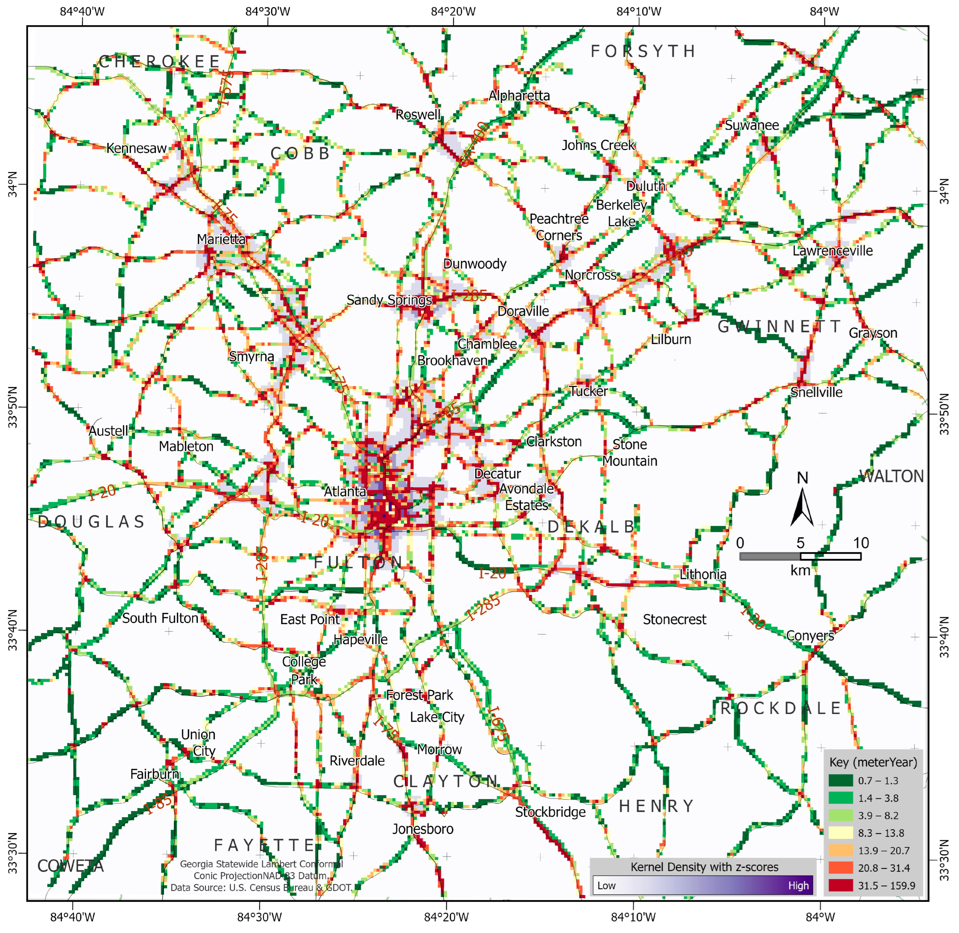
3.1. Temporal and Spatial Patterns

Temporal patterns were examined using the hourly congestion amounts, which were further summarized by day of the week and by hour. Figure 3 illustrates the results, measured in mileHours. The numbers in the legend key represent the average congestion amounts in mileHours. For example, “Sunday (86.4)” indicates that about 86.4 miles during an hour are congested in average on Sunday. Figure 3 reveals clear temporal patterns, with weekday congestion levels being significantly higher than those on weekends. Morning peaks are evident during weekdays, particularly around the 7–9 a.m. period, as commuters head to work or school, with Wednesday showing the sharpest rise. Similarly, an even more pronounced evening peak occurs between 4 and 6 p.m., likely due to this period being the end of the workday. Thursday shows the highest evening congestion, while Friday’s evening peak is slightly broader, indicating heavier or more extended traffic activity, possibly from people heading out for weekend plans. Overall, the traffic congestion amounts on Tuesday, Wednesday, and Thursday are similar to each other, with slight variations on Monday and Friday.

Weekend congestion levels remain consistently lower throughout the day, with no significant morning peak. Saturday exhibits a gradual increase in congestion, peaking modestly in the late afternoon, likely due to leisure or shopping activities. Sunday experiences the lowest congestion levels overall, with a flatter curve that peaks slightly in the afternoon. The average Sunday congestion amount of 86.4 mileHours, as shown in the legend, is about half of the peak days such as Wednesday, Thursday, or Friday.

Figure 4 shows the spatial distribution of annual congestion levels along major roads, measured in meterYear for individual 285 m pixels. The largest value is 159.9 meterYears, meaning that 159.9 m out of 285 m (approximately 56%) experience congestion throughout a year. High-congestion pixels, marked in red and dark red, are concentrated along major freeways, arterial roads, and their junctions, particularly in downtown Atlanta and its vicinity. Heavy congestion appears at the intersections of I–285 and I–20 west, I–75 north, GA–400, I–85 north, and I–20 east, which closely aligns with the truck bottlenecks reported by the American Transportation Research Institute [40]. Additionally, areas such as downtown and its northeastern region, as well as Alpharetta, Duluth, Norcross, Doraville, Smyrna, Decatur, and Marietta, experience heavy congestion. Significant outliers, where congestion amounts exceeded 50.0 meterYears, were notably observed on I–85 from Druid Hills to downtown, on I–285 at Sandy Springs, on I–285 north toward I–85 north in Doraville, on Georgia State Route 140 in Roswell, and in other scattered locations. Those outlier locations are included in the last category in Figure 4, where congestion is larger than 31.5 meterYears. Overall, the northern regions of I–20 experience more severe congestion compared to the southern areas. The figure also highlights congestion hotspots using dark purple tones, generated through kernel density calculations. Areas with heavy congestion patterns include downtown and its vicinity, Smyrna, Marietta, Sandy Springs, Brookhaven, Doraville, Duluth, Decatur, and Lawrenceville. Notably, the Sandy Springs area, where GA–400 intersects with I–285 North, has been prone to congestion for decades. Major construction projects in this area, known as the “Transform 400/285 Improvement Project,” began in 2017 (https://transform285400-gdot.hub.arcgis.com/, accessed on 24 November 2024) and overlapped with the study period, likely worsening the persistent heavy congestion observed there.

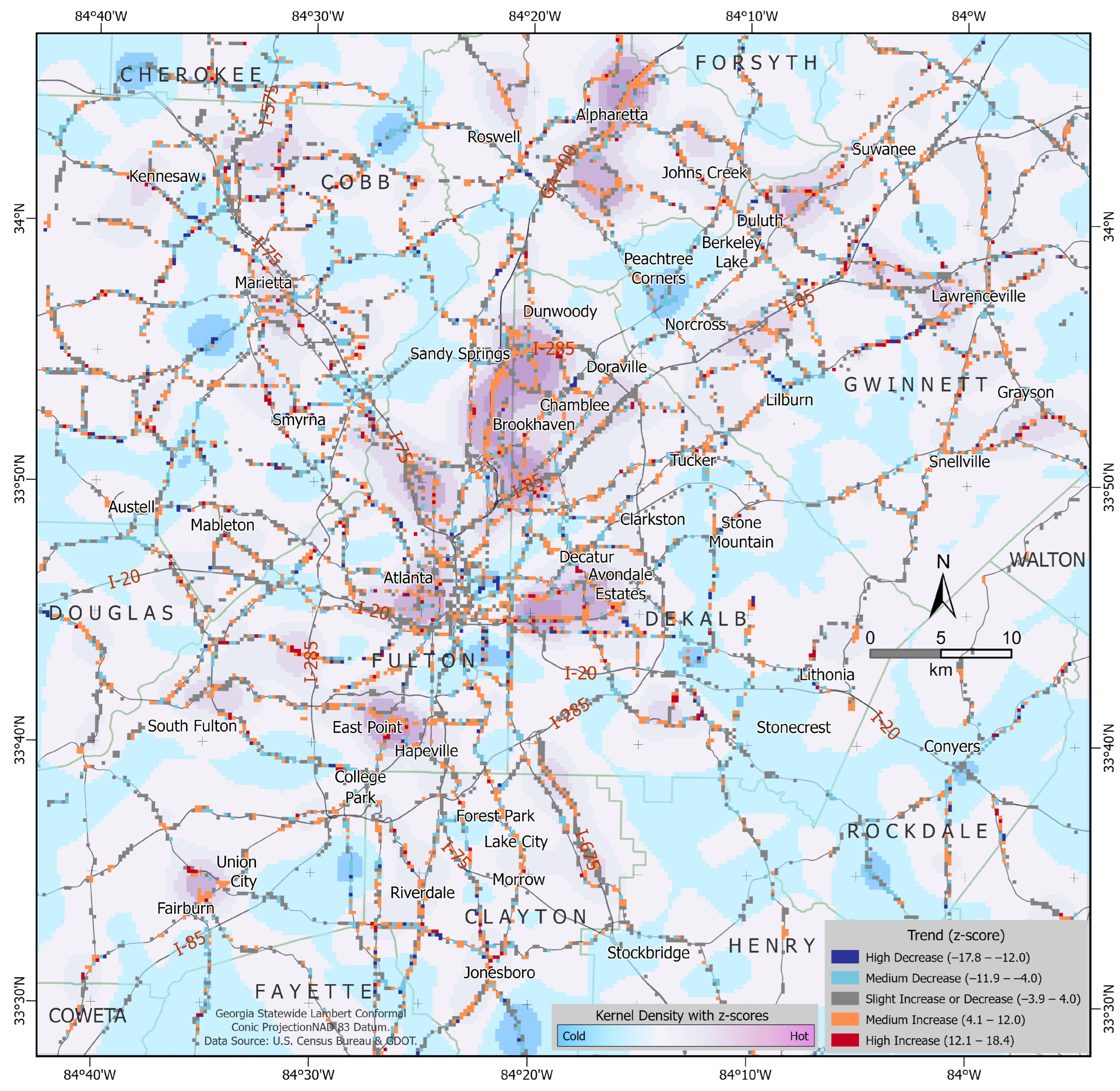
3.2. Temporal Trends

Figure 5 shows the results of the Mann–Kendall tests for individual pixels on roads. Pixels with increasing traffic congestion are highlighted in orange and red, while pixels with decreasing congestion are represented by blue tones. Significantly increasing trends are observed along major freeways, specifically on I–285 in the Sandy Springs area, I–85 near Suwanee, and at the I–575 and I–75 interchange. When a kernel density operation was applied using the z-score values at a pixel size of 350 m, hotspots of increasing congestion were identified in the Brookhaven–Sandy Springs corridor, the Druid Hills–Decatur corridor, the northwestern part of the city of Atlanta, the Johns Creek–Cumming corridor, the western part of the downtown area, and the East Point area. Remotely, the Fairburn and Union City areas also show increasing trends. Conversely, areas of decreasing congestion (cold spots) are found in the following locations: the southern neighbor of downtown, the eastern neighbor of downtown, the Peachtree Corners area, the eastern part of the I–20 and I–285 east intersection, and some remote suburban areas.

3.3. Regional Variations

Figure 6 shows annual traffic congestion amounts in various cities in the metro Atlanta area, summarized in terms of the annual average daily congestion (AADC) in mileDays. The city of Atlanta has the highest congestion (26 mileDays), shown in deep red, indicating that an average of 26 miles experience traffic congestion for 24 h. The congestion amount in the city of Atlanta is about five times higher than that in the next tier of cities (i.e., Roswell, Marietta, Sandy Springs, and South Fulton).

Considering that the downtown area has the highest road density, the annual total congestion amounts appear to be influenced by road density in the study area. When the congestion amounts were normalized by the road lengths in individual cities (see, Figure 7), Dunwoody, Norcross, Decatur, and Jonesboro show the heaviest congestion per road distance, followed by Marietta, the city of Atlanta, Sandy Springs, Smyrna, Lilburn, Lawrenceville, Snellville, Avondale Estates, and Riverdale.

Figure 8 shows the results of the Mann–Kendall test, which reveals trends in traffic congestion over time. The positive z-scores in warm colors indicate a trend of increasing congestion, while negative z-scores shown in blue represent areas with decreasing congestion. Gray areas indicate the regions where trends were not statistically significant. Cities such as Alpharetta, Dunwoody, Brookhaven, Austell, Stone Mountain, East Point, Lake City, Morrow, Fairburn, and Jonesboro show high increasing trends in congestion, highlighted in dark red. Johns Creek, Duluth, Lawrenceville, the city of Atlanta, Decatur, Hapeville, and Clarkston show moderate increasing trends. Conversely, a moderate decreasing trend appears in Lilburn. Cities like Conyers and Forest Park show high decreasing trends, shaded in blue. Among 43 cities, 23 cities do not show significant trends, 17 cities show increasing trends, and 3 cities show decreasing trends. Figure 8 also shows that the kernel density hotspots, identified in Figure 5, align well with the heavy increase in Figure 8 or with the heavily congested cities in Figure 6.

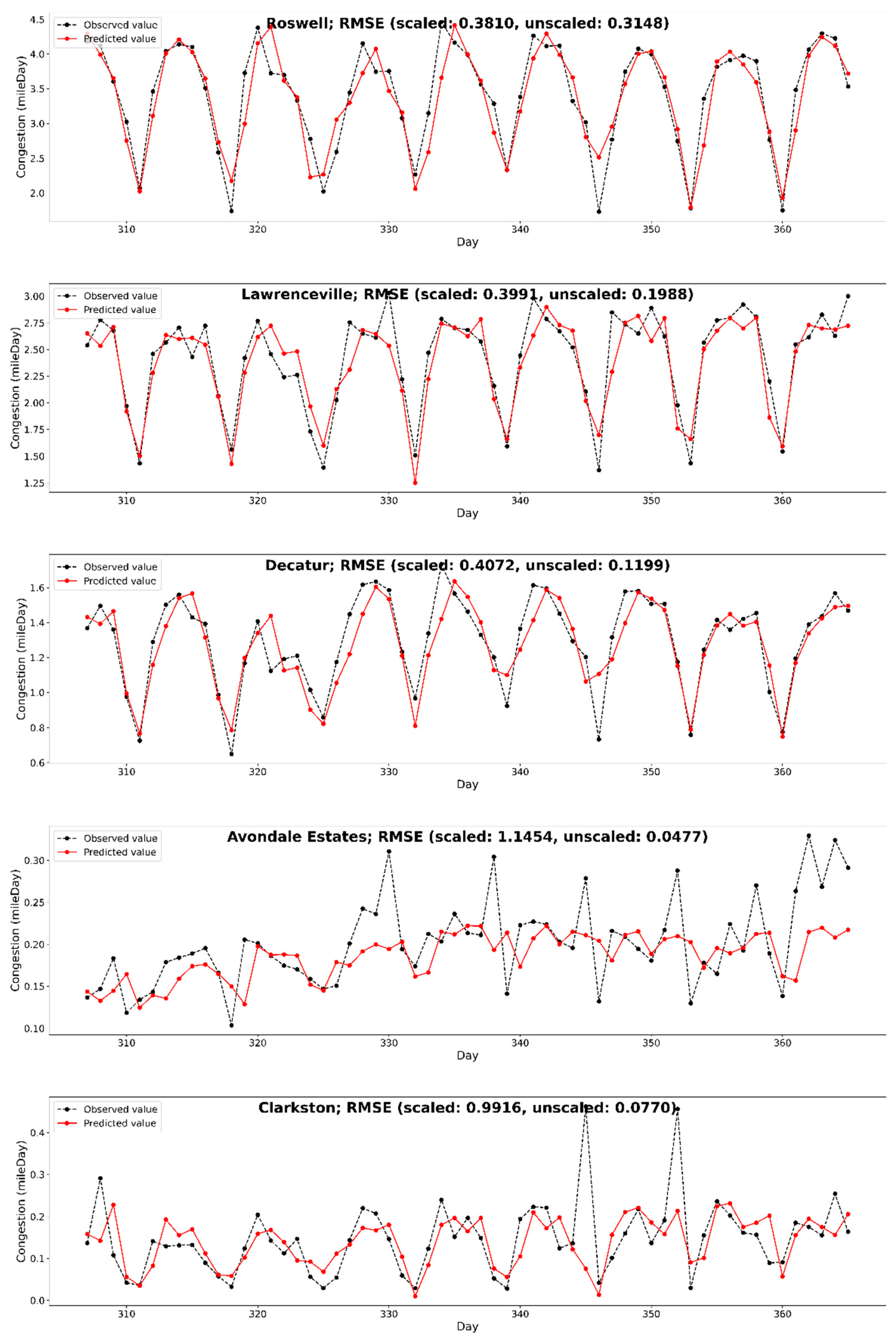
3.4. Predicted Trends

Table 1. LSTM model hyperparameters and RMSE with test dataset.

City	Hidden Nodes	Hidden Layers	Learning Rate	Epochs	Validation Loss (MSE)	Test Loss (RMSE)
=Alpharetta	32	3	0.001	10	0.5166	0.7514
Atlanta	32	3	0.001	50	0.4699	0.5882
Austell	64	3	0.001	50	0.1744	0.6153
Avondale Estates	32	3	0.001	30	0.5011	1.1454
Berkeley Lake	32	2	0.001	50	0.3281	0.4386
Brookhaven	64	3	0.001	10	0.2856	0.6604
Chamblee	32	3	0.001	10	0.3629	0.7643
Clarkston	64	3	0.001	50	0.4368	0.9916
College Park	32	3	0.001	10	0.3440	0.8407
Conyers	64	1	0.001	50	0.2763	0.4838
Decatur	64	3	0.001	50	0.4953	0.4072
Doraville	64	2	0.001	50	0.3425	0.5002
Duluth	64	3	0.001	30	0.3166	0.4143
Dunwoody	64	2	0.001	30	0.2611	0.6023
East Point	32	3	0.001	10	0.0834	0.7783
Fairburn	64	1	0.001	50	0.3219	0.9189
Forest Park	64	3	0.001	50	0.2174	0.4509
Grayson	32	1	0.001	50	0.9174	0.5089
Hapeville	32	1	0.001	30	3.5845	0.5690
Johns Creek	64	2	0.001	30	0.2328	0.4692
Jonesboro	32	2	0.001	10	0.4641	0.5824
Kennesaw	64	2	0.001	10	0.4040	0.4689
Lake City	64	1	0.001	10	0.4584	0.7992
Lawrenceville	64	2	0.001	50	0.1322	0.3991
Lilburn	64	3	0.001	30	0.1656	0.5162
Lithonia	64	3	0.001	50	0.2241	0.6889
Mableton	64	2	0.001	30	0.3516	0.5291
Marietta	32	2	0.001	50	0.3235	0.7732
Morrow	32	1	0.001	10	0.6072	0.8320
Norcross	32	3	0.001	30	0.4845	0.4294
Peachtree Corners	32	1	0.001	50	0.3721	0.4398
Riverdale	64	3	0.001	50	0.4331	0.6334
Roswell	32	3	0.001	50	0.1941	0.3810
Sandy Springs	64	1	0.001	50	0.2399	0.4413
Smyrna	64	1	0.001	50	0.4179	0.5925
Snellville	64	3	0.001	30	0.2003	0.5568
South Fulton	64	2	0.001	50	0.0873	0.5208
Stockbridge	32	3	0.001	50	0.3996	0.7355
Stone Mountain	32	1	0.001	50	0.2845	0.5909
Stonecrest	32	2	0.001	50	0.2060	0.9212
Suwanee	64	3	0.001	10	0.6972	0.7017
Tucker	64	3	0.001	10	0.4993	0.4598
Union City	32	1	0.001	10	0.2348	0.7230

shows a summary of the LSTM model’s performance across different cities with the hyperparameters suggested by the Optuna library. The root mean square error (RMSE) values of the loss values of the test datasets highlight the predictive accuracy of the LSTM models across cities. In the table, the MSE and RMSE values were calculated from the scaled values using standard scores. Cities like Roswell, Lawrenceville, Decatur, and Duluth show relatively lower RMSE values, indicating accurate predictions. Conversely, cities like Avondale Estates, Clarkston, Stonecrest, and Fairburn show higher RMSE values, suggesting a need for further tuning or that the data may have higher variability. The RMSE of Avondale is about four times larger than that of Roswell. ANOVAs (Analyses of Variance) were performed to check whether the number of hidden nodes, hidden layers, or epochs affects the test RMSE values, and the results show that they do not significantly affect the test RMSE value with the p-values of 0.077 for hidden nodes, 0.499 for hidden layers, and 0.210 for epochs.

Figure 9 shows examples of model performance by comparing the predicted values to the actual values for the cities with the smallest (i.e., Roswell, Lawrenceville, and Decatur) and largest (i.e., Avondale Estates and Clarkston) RMSE values. The larger RMSE values indicate poor prediction performances. The test RMSE values are displayed in the figure, with scaled RMSE values representing standard scores and unscaled RMSE values reflecting the original measurements. As shown in the plots, the LSTM predictions show significant discrepancies, especially during sudden spikes or sharp changes in the actual data. These deviations imply the LSTM model’s difficulty in adapting to abrupt transitions, or limitations in hyperparameter tuning for those abrupt changes.

4. Discussion

This study analyzed traffic congestion in Metro Atlanta, focusing on regional and temporal patterns, trends, and predictive modeling to enhance urban planning. As noted by multiple studies [41,42,43], significant weekday congestion amounts were much higher than those on weekends, with peaks in the morning and afternoon. Congestion hotspots concentrated along major freeways and intersections, particularly in the downtown area and above. Tuesday, Wednesday, and Thursday congestion amounts were similar to each other, while the Sunday amount was about half of those days. Geographically, the northern part of I–20 showed much heavier traffic congestion when compared with the southern part of I–20.

The increasing trend of traffic congestion along the Brookhaven–Sandy Springs corridor and along the Johns Creek–Cumming corridor matches very well with the recent developments in those areas [44,45]. Furthermore, the increasing trend in the Druid Hills–Decatur corridor, well known for recent gentrification alongside the Atlanta Beltline projects near Ponce City Market and Emory University [46], appears to reflect the area’s rapid urban development without a corresponding expansion in transportation infrastructure capacity. It is, however, quite unusual to observe a cold spot in the Peachtree Corners area. Given that this region has also undergone significant urban development, characterized by townhomes, mixed-use condominiums, and upscale shopping complexes like the Forum Mall, further investigation into the Peachtree Corners area is warranted.

When comparing the city-wise congestion trends in Figure 8 with the pixel-wise trends in Figure 5, both maps notably highlight congestion corridors in areas such as Brookhaven–Dunwoody, Johns Creek–Cumming, Druid Hills–Decatur, East Point, and Fairburn. However, the map does not capture the cold spots near downtown and Peachtree Corners. Overall, the city-wise trends effectively represent congestion changes. The increasing congestion spots align with the ARC MTP’s focus on major roadway projects primarily outside of the I–285 loop, particularly on the north and east sides. Figure 8 shows that there are five high increasing cities in the north of I–20. The same number of high increasing cities also appear in the south of I–20. This implies that the ARC’s Capacity Projects described in the 2050 MTP report [11] might need to pay more attention to the high increasing communities in the southern part of Metro Atlanta.

This research also demonstrated that predictive modeling using LSTM and distanceTime measurements performs well for short-term predictions in most cities. However, some cities require additional tuning due to data variability, such as sudden peaks or drops. With further hyperparameter optimization, the model’s performance can improve significantly, and future research will focus on these enhancements. Overall, the hyperparameter generation algorithm provided by Optuna library performed exceptionally well, especially given its ease of implementation.

This research provides some valuable insights into traffic congestion analysis. First, the distanceTime measurement proves to be an effective tool for summarizing regional traffic congestion in diverse ways. Second, the Mann–Kendall test is a robust method for identifying congestion in hot and cold spots using pixel-level or city-wise datasets. Third, automated hyperparameter optimization algorithms, such as Optuna, generally perform well, although they may struggle with modeling sudden spikes or drops. Finally, regionally summarized congestion levels, trends, and patterns can serve as important resources for urban planners and policymakers.

5. Conclusions

This study provides a comprehensive analysis of traffic congestion from a regional perspective in Metro Atlanta, highlighting significant temporal and spatial patterns, regional variations, and trends. The results show that weekday congestion levels are substantially higher than weekend traffic, with pronounced morning and evening peaks, especially on major freeways and in downtown Atlanta. Geographically, congestion is most severe in the northern parts of I–20 and, particularly, at the key urban corridors such as Brookhaven–Sandy Springs, the downtown connector, Druid Hills–Decatur, and Johns Creek–Cumming, aligning with recent urban developments in those regions. Even though the cities of Atlanta, Marietta, Roswell, Sandy Springs, and South Fulton show high annual average daily congestion amounts, the normalized map by city-wise road length shows heavier congestion in Dunwoody, Norcross, Decatur, and Jonesboro, which implies heavier congestion on their major roads. Cities such as Alpharetta, Dunwoody, Brookhaven, Austell, Stone Mountain, East Point, Lake City, Morrow, Fairburn, and Jonesboro exhibit significant increases in congestion. Johns Creek, Duluth, Lawrenceville, the city of Atlanta, Decatur, Hapeville, and Clarkston show moderate increases in congestion. In contrast, Lilburn experiences a moderate decrease. Conyers and Forest Park are among the cities with significant decreases. Out of 43 cities, 23 show no notable trends, 17 exhibit increasing trends, and 3 show decreasing trends. Furthermore, predictive modeling using LSTM shows promising results for short-term forecasts, though variability in data requires further optimization for certain cities. The findings in this research demonstrate that distanceTime metrics may be used as an effective tool to measure congestion amounts to support not only road-wise analyses but also regional city-wise summarization and analyses. The methodologies and regional insights from this research might aid urban planning and policymaking, particularly in identifying areas with high or growing congestion, and in guiding transportation infrastructure improvements.

References

1. Federal Highway Administration. Traffic Congestion and Reliability: Linking Solutions to Problems. 2004. Available online: https://ops.fhwa.dot.gov/congestion_report_04/index.htm (accessed on 27 November 2024).
2. Hennessy, D.A. Social, Personality, and Affective Constructs in Driving. In Handbook of Traffic Psychology; Porter, B., Ed.; Elsevier: Amsterdam, The Netherlands, 2011; pp. 149–164. [Google Scholar] [CrossRef]
3. Noratikah, W.; Ghazali, B.W.; Nurhamizah, C.; Zulkifli, A.B.; Ponrahomo, Z. The Effect of Traffic Congestion on Quality of Community Life. In Proceedings of the ICRP 2019—4th International Conference on Rebuilding Place, George Town, Malaysia, 6–7 November 2019. [Google Scholar] [CrossRef]
4. Beckmann, M.J. Traffic Congestion and What to Do About It. Transp. B Transp. Dyn. 2013, 1, 103–109. [Google Scholar] [CrossRef]
5. Khalid, A.; Vaughn, C. Application of System Selection Tool to Traffic Congestion in Metro Atlanta: A Case Study. In Proceedings of the 2011 ASEE Annual Conference & Exposition, Vancouver, BC, Canada, 26–29 June 2011. [Google Scholar] [CrossRef]
6. Kumar, M.; Kumar, K.; Das, P. Study on Road Traffic Congestion: A Review. In Recent Trends in Communication and Electronics; CRC Press: Boca Raton, FL, USA, 2021; pp. 230–240. [Google Scholar] [CrossRef]
7. Duranton, G.; Turner, M.A. The Fundamental Law of Road Congestion: Evidence from US Cities. Am. Econ. Rev. 2011, 101, 2616–2652. [Google Scholar] [CrossRef]
8. Mann, A. What’s Up with That: Building Bigger Roads Actually Makes Traffic Worse. WIRED, 17 June 2014. Available online: https://www.wired.com/2014/06/wuwt-traffic-induced-demand/ (accessed on 27 November 2024).
9. Djahel, S.; Doolan, R.; Muntean, G.-M.; Murphy, J. A Communications-Oriented Perspective on Traffic Management Systems for Smart Cities: Challenges and Innovative Approaches. IEEE Commun. Surv. Tutor. 2015, 17, 125–151. [Google Scholar] [CrossRef]
10. Afrin, T.; Yodo, N. A Survey of Road Traffic Congestion Measures Towards a Sustainable and Resilient Transportation System. Sustainability 2020, 12, 4660. [Google Scholar] [CrossRef]
11. Atlanta Regional Commission. 2050 Metropolitan Transportation Plan. 2024. Available online: https://atlantaregional.org/what-we-do/transportation-planning/metropolitan-transportation-plan/ (accessed on 27 November 2024).
12. Delaware Valley Regional Planning Commission. Congestion Management Process. 2023. Available online: https://www.dvrpc.org/reports/24135.pdf (accessed on 27 November 2024).
13. Code of Federal Regulations. Title 23—Highways. Available online: https://www.ecfr.gov/current/title-23/chapter-I/subchapter-E/ (accessed on 27 November 2024).
14. Zhang, K.; Sun, D.; Shen, S.; Zhu, Y. Analyzing Spatiotemporal Congestion Patterns on Urban Roads Based on Taxi GPS Data. J. Transp. Land Use 2017, 10, 675–694. [Google Scholar] [CrossRef]
15. National Academies of Sciences, Engineering, and Medicine. Prioritization of Public Transportation Investments: A Guide for Decision-Makers; TCRP Research Report 227 for TCRP Project H-58; The National Academies Press: Washington, DC, USA, 2021. [Google Scholar] [CrossRef]
16. Rahman, M.M.; Najaf, P.; Fields, M.G.; Thill, J.C. Traffic Congestion and Its Urban Scale Factors: Empirical Evidence from American Urban Areas. Int. J. Sustain. Transp. 2021, 16, 406–421. [Google Scholar] [CrossRef]
17. Lomax, T.; Turner, S.; Shunk, G. NCHRP Report 398: Quantifying Congestion: Volume 1—Final Report; Transportation Research Board, National Research Council: Washington, DC, USA, 1997. Available online: http://onlinepubs.trb.org/onlinepubs/nchrp/nchrp_rpt_398.pdf (accessed on 21 January 2025).
18. INRIX. 2023 INRIX Global Traffic Scorecard. 2024. Available online: https://inrix.com/scorecard/ (accessed on 27 November 2024).
19. Google. Google Maps Platform. Available online: https://developers.google.com/maps/documentation/routes/compute_route_directions (accessed on 27 November 2024).
20. Wang, F.; Xu, Y. Estimating O–D Travel Time Matrix by Google Maps API: Implementation, Advantages, and Implications. Ann. GIS 2011, 17, 199–209. [Google Scholar] [CrossRef]
21. Marasco, D.; Murray-Tuite, P.; Guikema, S.; Logan, T. Time to Leave: An Analysis of Travel Times During the Approach and Landfall of Hurricane Irma. Nat. Hazards 2020, 103, 2459–2487. [Google Scholar] [CrossRef]
22. Zafar, N.; Ul Haq, I. Traffic Congestion Prediction Based on Estimated Time of Arrival. PLoS ONE 2020, 15, e0238200. [Google Scholar] [CrossRef]
23. Gong, F.-Y. Modeling Walking Accessibility to Urban Parks Using Google Maps Crowdsourcing Database in the High-Density Urban Environments of Hong Kong. Sci. Rep. 2023, 13, 20798. [Google Scholar] [CrossRef]
24. Seong, J.; Kim, Y.; Goh, H.; Kim, H.; Stanescu, A. Measuring Traffic Congestion with Novel Metrics: A Case Study of Six U.S. Metropolitan Areas. ISPRS Int. J. Geo-Inf. 2023, 12, 130. [Google Scholar] [CrossRef]
25. Kim, Y. Prediction of Traffic Congestion Using a Time-Series Model and Spatiotemporal Data: A Case Study of the Atlanta Downtown Connector. Geogr. Bull. 2023, 64, 93–102. Available online: https://digitalcommons.kennesaw.edu/thegeographicalbulletin/vol64/iss2/7 (accessed on 27 November 2024).
26. Ji, S.; Seong, J.; Stanescu, A.; Hwang, C.S.; Lee, Y. Spatiotemporal Traffic Database Construction with Google Real-Time Traffic Information and Spatiotemporal Congestion Pattern Analysis: A Case Study of Montgomery County, Maryland, U.S.A. J. Korean Geogr. Soc. 2021, 56, 265–276. [Google Scholar] [CrossRef]
27. ESRI. How Kernel Density Works. ArcGIS Pro 3.4 Reference Manual. Available online: https://pro.arcgis.com/en/pro-app/latest/tool-reference/spatial-analyst/how-kernel-density-works.htm (accessed on 27 November 2024).
28. Silverman, B.W. Density Estimation for Statistics and Data Analysis; Chapman and Hall: London, UK, 1986; 175p. [Google Scholar] [CrossRef]
29. Hirsh, R.M.; Slack, J.R.; Smith, R.A. Techniques of Trend Analysis for Monthly Water-Quality Data. Water Resour. Res. 1982, 18, 107–121. [Google Scholar] [CrossRef]
30. Helsel, D.R.; Mueller, D.K.; Slack, J.R. Computer Program for the Kendall Family of Trend Tests; U.S. Geological Survey: Reston, VA, USA, 2006. Available online: https://pubs.usgs.gov/sir/2005/5275/pdf/sir2005-5275.pdf (accessed on 27 November 2024).
31. U.S. Bureau of the Census. Geographic Areas Reference Manual. 1994. Available online: https://purl.fdlp.gov/GPO/LPS53335 (accessed on 27 November 2024).
32. U.S. Bureau of the Census. TIGER Geodatabases. 2023. Available online: https://www.census.gov/geographies/mapping-files/time-series/geo/tiger-geodatabase-file.html (accessed on 27 November 2024).
33. Hochreiter, S.; Schmidhuber, J. Long Short-Term Memory. Neural Comput. 1997, 9, 1735–1780. [Google Scholar] [CrossRef]
34. Akhtar, M.; Moridpour, S. A Review of Traffic Congestion Prediction Using Artificial Intelligence. J. Adv. Transp. 2021, 2021, 8878011. [Google Scholar] [CrossRef]
35. Giles, C.L.; Lawrence, S.; Tsoi, A.C. Noisy Time Series Prediction Using Recurrent Neural Networks and Grammatical Inference. Mach. Learn. 2001, 44, 161–183. [Google Scholar] [CrossRef]
36. Xu, F. Research on Traffic Flow Prediction Method Based on LSTM Model and PSO-LSTM Model. Appl. Comput. Eng. 2024, 101, 154–163. [Google Scholar] [CrossRef]
37. Mojtaba, M.; Abdoul-Ahad, C.; Farshid, A. The Short-Term Prediction of Daily Traffic Volume for Rural Roads Using Shallow and Deep Learning Networks: ANN and LSTM. J. Supercomput. 2023, 79, 17475–17494. [Google Scholar] [CrossRef]
38. Scikit-Learn. StandardScaler. Available online: https://scikit-learn.org/1.5/modules/generated/sklearn.preprocessing.StandardScaler.html (accessed on 27 November 2024).
39. Akiba, T.; Sano, S.; Yanase, T.; Ohta, T.; Koyama, M. Optuna: A Next-Generation Hyperparameter Optimization Framework. In Proceedings of the 25th ACM SIGKDD International Conference on Knowledge Discovery and Data Mining, Anchorage, AK, USA, 4–8 August 2019. [Google Scholar] [CrossRef]
40. American Transportation Research Institute. Top 100 Truck Bottlenecks—2023. Available online: https://truckingresearch.org/2023/02/top-100-truck-bottlenecks-2023/ (accessed on 27 November 2024).
41. Almatar, K.M. Traffic Congestion Patterns in the Urban Road Network: (Dammam Metropolitan Area). Ain Shams Eng. J. 2023, 14, 101886. [Google Scholar] [CrossRef]
42. Wei, X.; Ren, Y.; Shen, L.; Shu, T. Exploring the Spatiotemporal Pattern of Traffic Congestion Performance of Large Cities in China: A Real-Time Data-Based Investigation. Environ. Impact Assess. Rev. 2022, 95, 106808. [Google Scholar] [CrossRef]
43. Agarwal, A. A Comparison of Weekend and Weekday Travel Behavior Characteristics in Urban Areas. USF Tampa Graduate Theses and Dissertations, University of South Florida, Tampa, FL, USA, 2004. Available online: https://digitalcommons.usf.edu/etd/936 (accessed on 12 November 2024).
44. Perimeter Community Improvement Districts. Consolidated Plan: Perimeter in Progress, 2021 Update. 2021. Available online: https://perimeteratl.com/wp-content/uploads/2023/11/PCID-2021-Consolidated-Plan-Final-compressed.pdf (accessed on 27 November 2024).
45. City of Cumming, Georgia. Comprehensive Plan 2022–2042. 2022. Available online: https://www.cityofcumming.net/wp-content/uploads/2022/10/Cumming-Comp-Plan-Adopted-10-4-2022.pdf (accessed on 27 November 2024).
46. Byahut, S.; Ghosh, S.; Masilela, C. Urban Transformation for Sustainable Growth and Smart Living: The Case of the Atlanta Beltline. In Smart Living for Smart Cities; Springer Nature: Singapore, 2020; Chapter 13. [Google Scholar] [CrossRef]
Figure 1. The study area in Metro Atlanta, Georgia, with cities shown in unique background colors. The section where I–75 and I–85 run together from A to B is known as the “downtown connector”.
Ijgi 14 00061 g001
Figure 2. A schematic diagram of the workflow performed in this research.
Ijgi 14 00061 g002
Figure 3. Temporal congestion amounts by day of the week and hour. The number in the legend key indicates the average congestion amount for the day.
Ijgi 14 00061 g003
Figure 4. Annual congestion amount in each pixel.
Ijgi 14 00061 g004
Figure 5. Mann–Kendall test results at individual pixels.
Ijgi 14 00061 g005
Figure 6. Traffic congestion amounts in the Metro Atlanta cities measured by annual average daily congestion (AADC).
Ijgi 14 00061 g006
Figure 7. Normalized congestion amounts. The annual average daily congestion amounts were divided by the road lengths in miles at each city to calculate the normalized congestion amounts.
Ijgi 14 00061 g007
Figure 8. Mann–Kendall test results in individual cities.
Ijgi 14 00061 g008
Figure 9. Examples of LSTM model performances showing predicted values (red lines) against observed values (black lines). Shown here are 5 sample cities among 43 cities.
Ijgi 14 00061 g009