

VE-GCN: A Geography-Aware Approach for Polyline Simplification in Cartographic Generalization


Abstract
:1. Introduction
- (1)
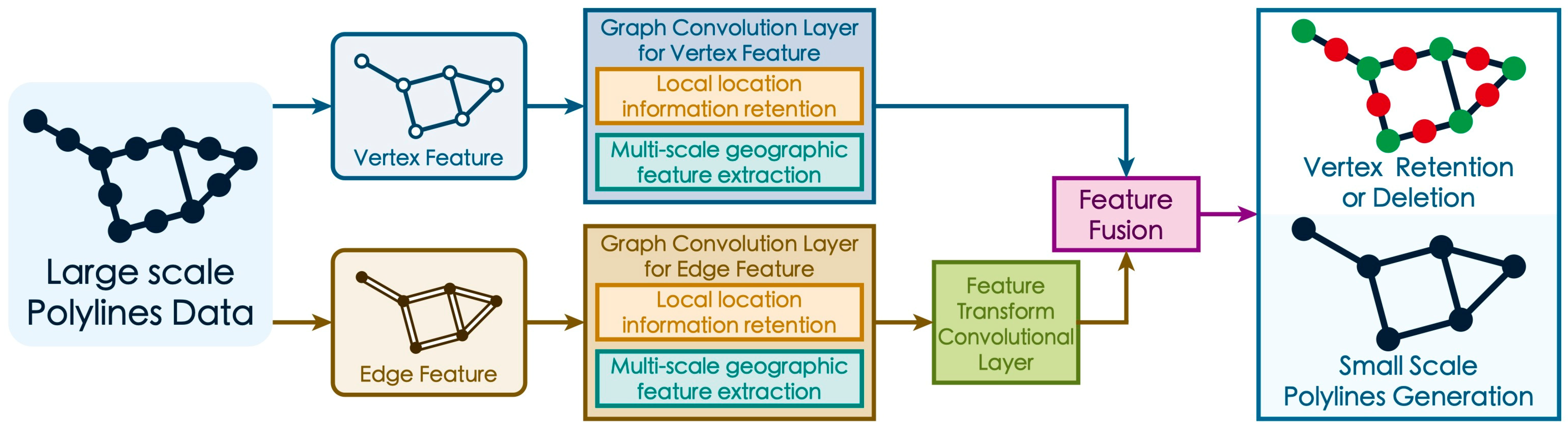
- Limitations of vertex features: In graph structures, edges represent connections between vertices and lack physical entities. However, in map polylines, edges are also fundamental elements. Cartographic generalization is a constrained, cognition-driven process guided by thinking, and intelligent polyline simplification should fully consider the geometric and geographic properties of both vertices and edges to better express cognitive rules and cartographic principles.
- (2)
- Extraction of crucial geographic features: Geographical features refer to the composition, distribution, and interrelationships of the geographic elements in an area. Due to the lack of directional properties in graph convolutional kernels, unlike raster convolutional kernels, graph convolutional layers merely aggregate information. This results in graph convolutional models having a lower capacity to learn features compared to convolutional networks.
2. Related Works
2.1. Geometry-Based Simplification Methods
2.2. Machine-Learning-Based Simplification Methods
3. Materials and Methods
3.1. Improved Graph Convolutional Layer for Geographic Structure
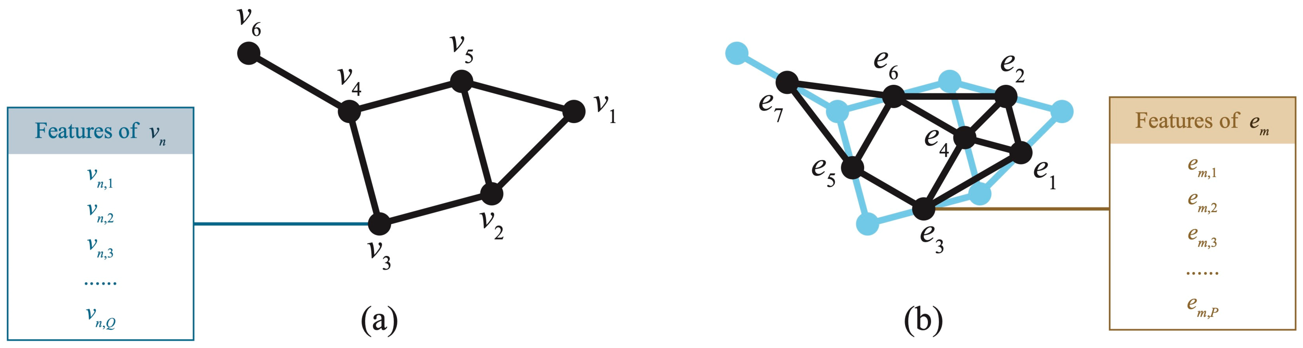
3.1.1. Construction of Geographic Graph Structure
3.1.2. Integration of Vertex and Edge Features
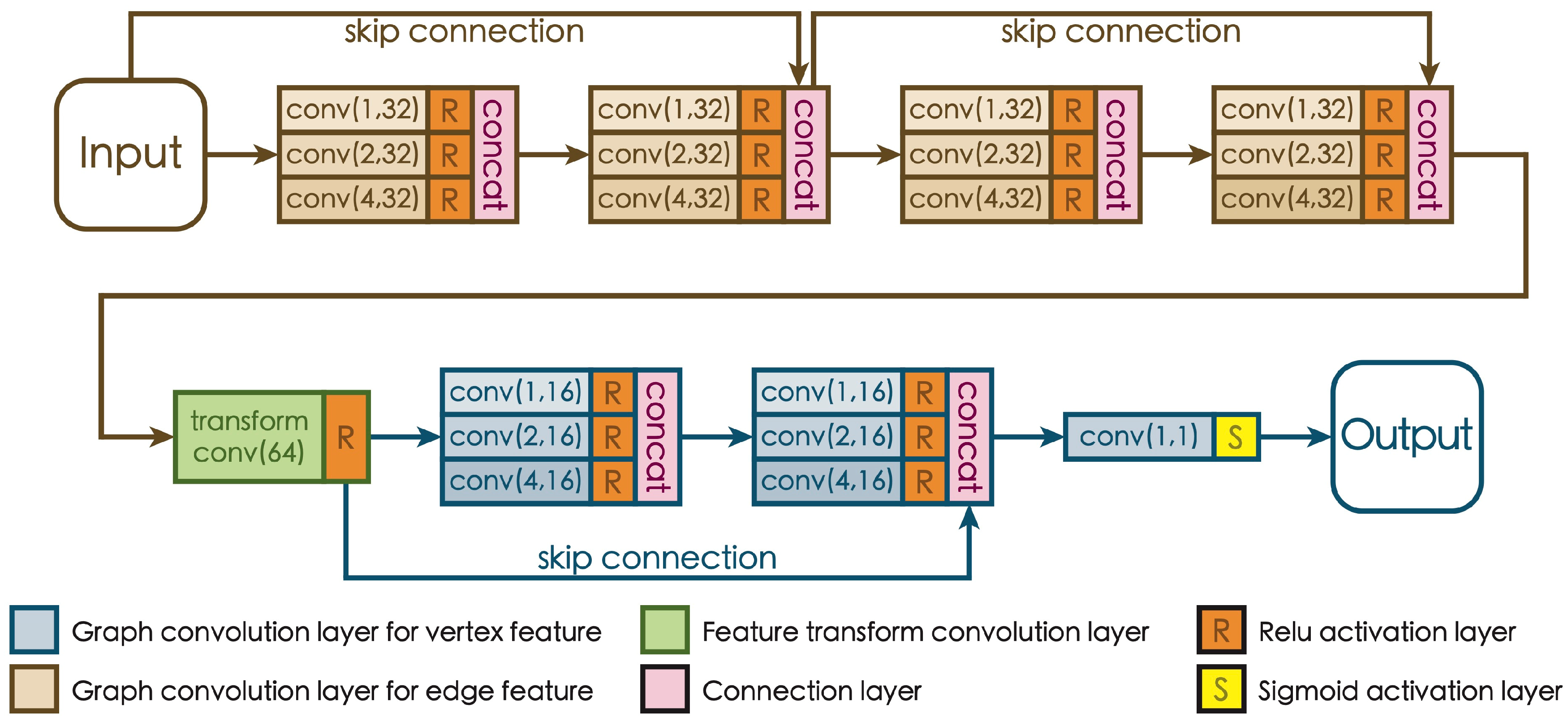
3.2. Architecture for Retaining Crucial Geographic Features
3.2.1. Structure for Retaining Local Positional Information
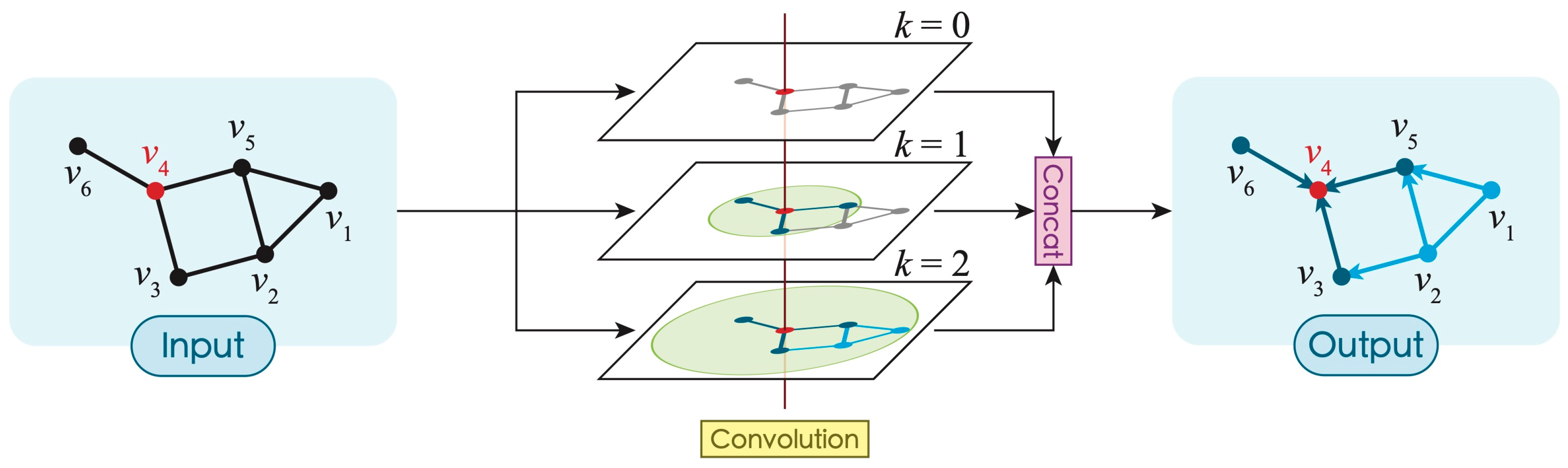
3.2.2. Structure for Extracting Multi-Scale Geographic Information
3.3. Loss Function
4. Experiments
4.1. Evaluation Metrics
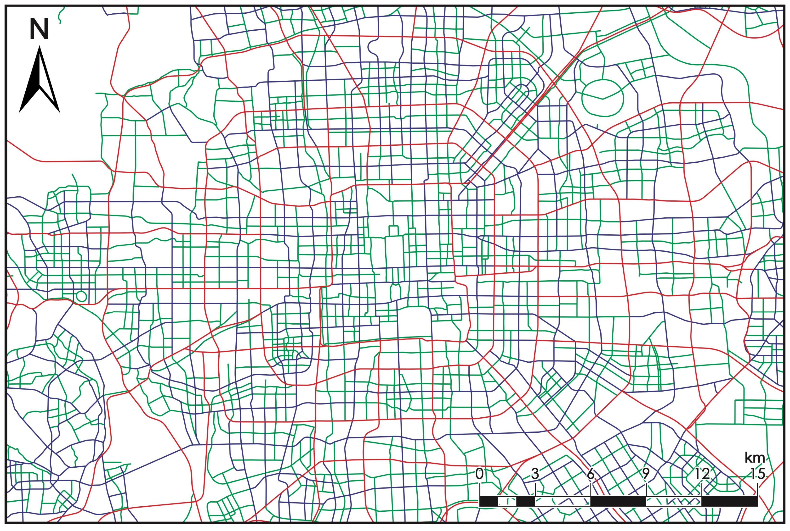
4.2. Road Simplification Experiment
4.2.1. Data Source
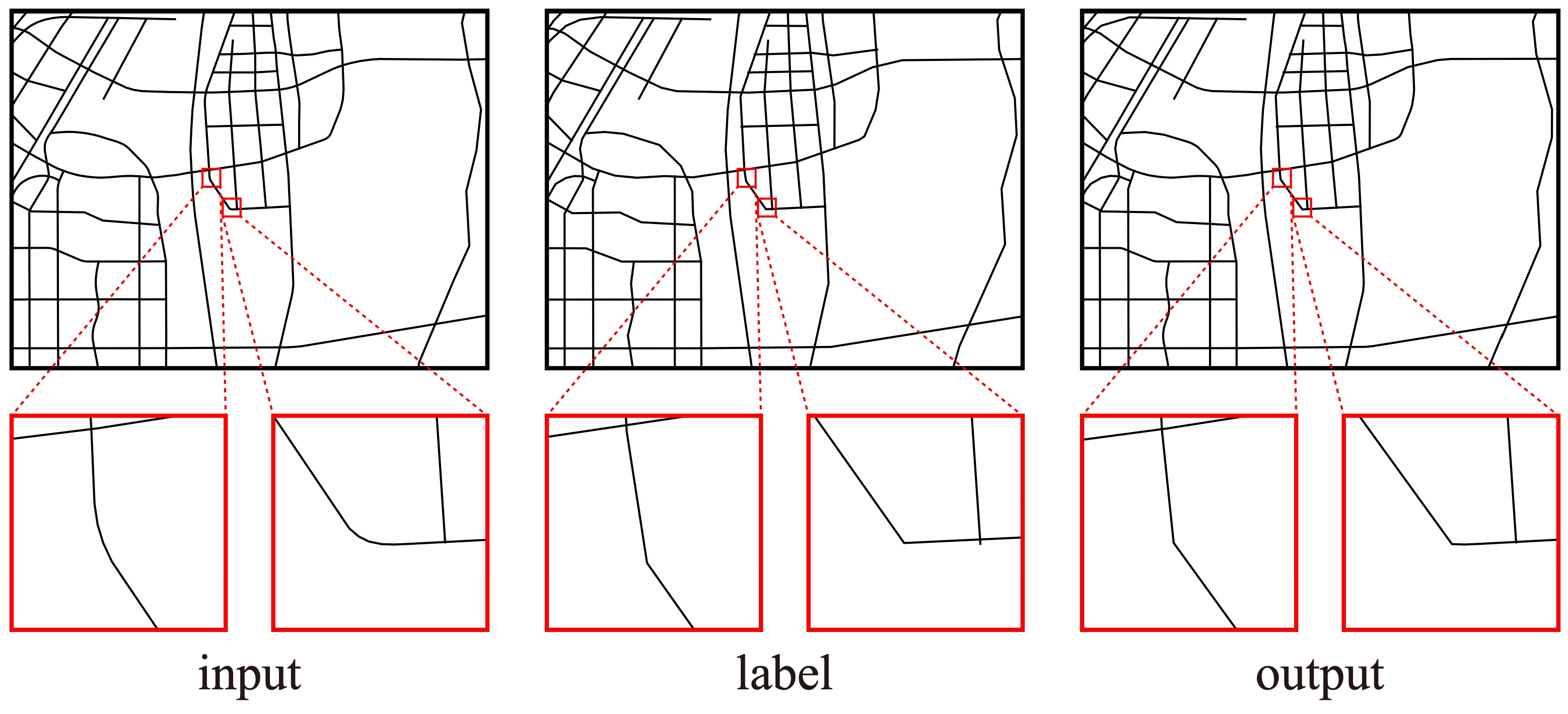
4.2.2. Result
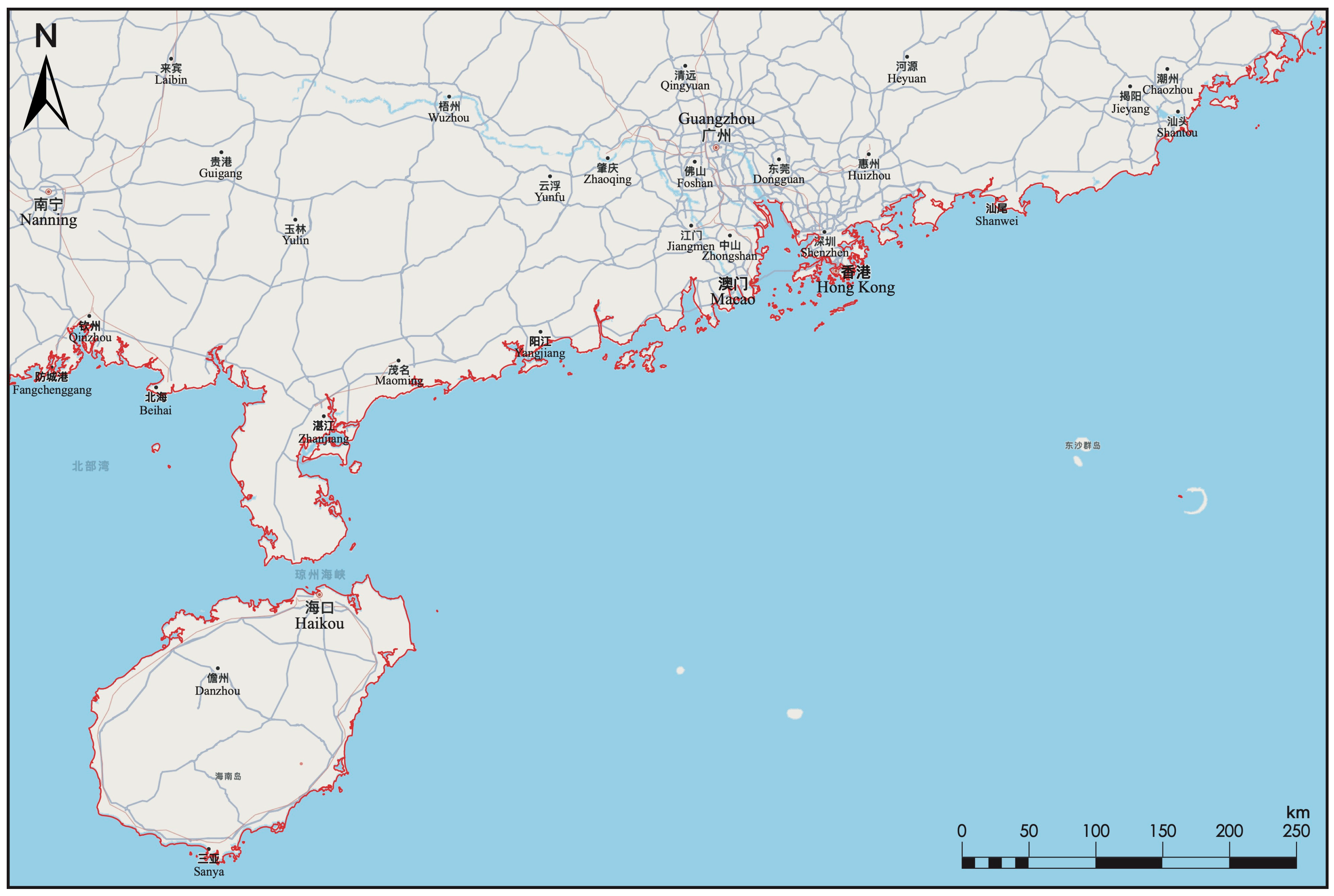
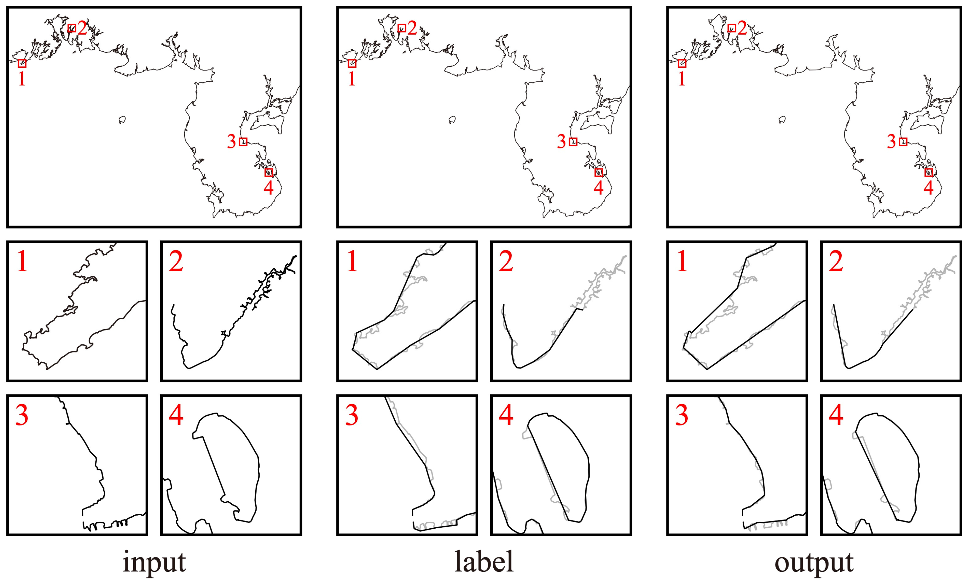
4.3. Coastline Simplification Experiment
4.3.1. Data Source and Processing
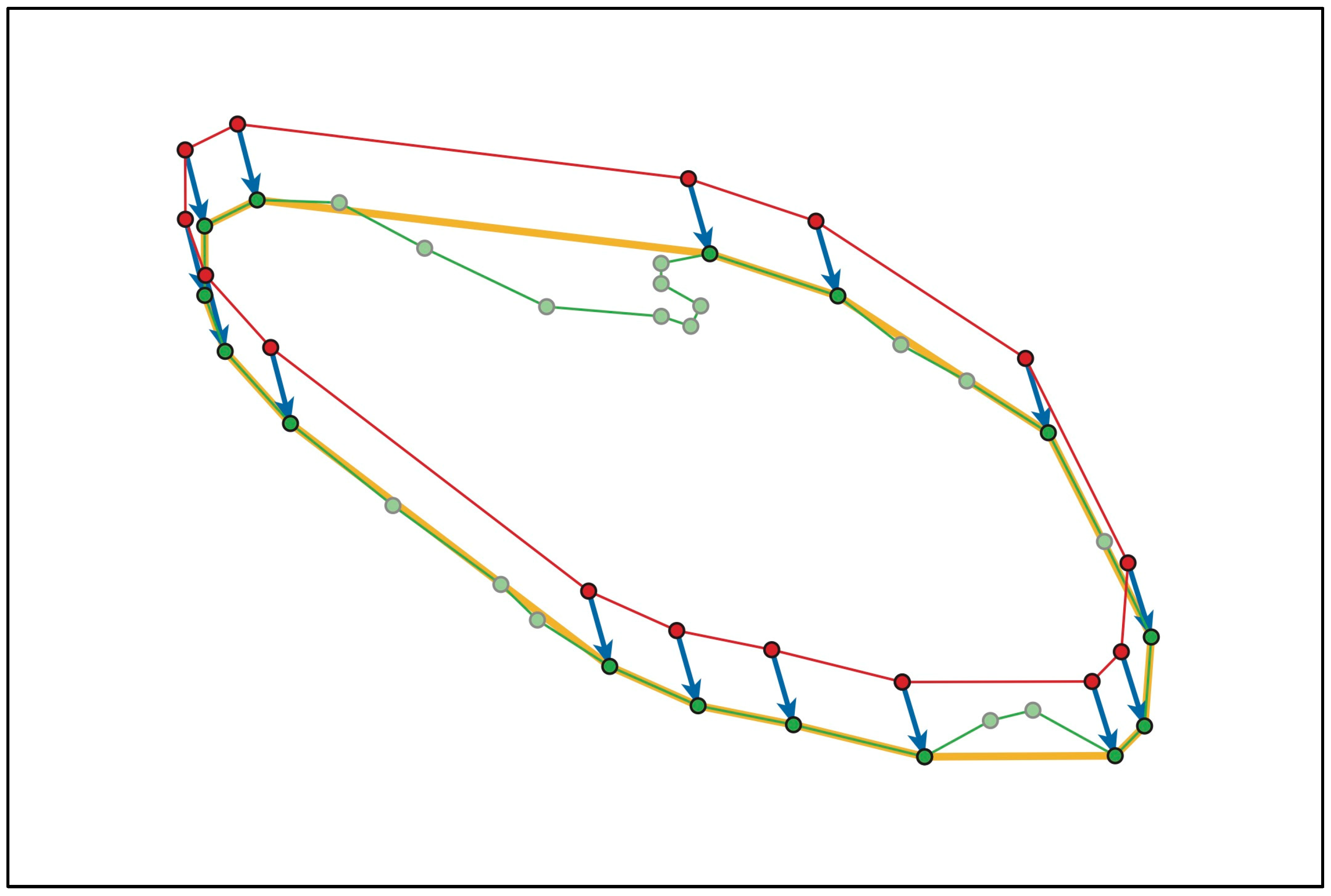
4.3.2. Result
5. Discussion
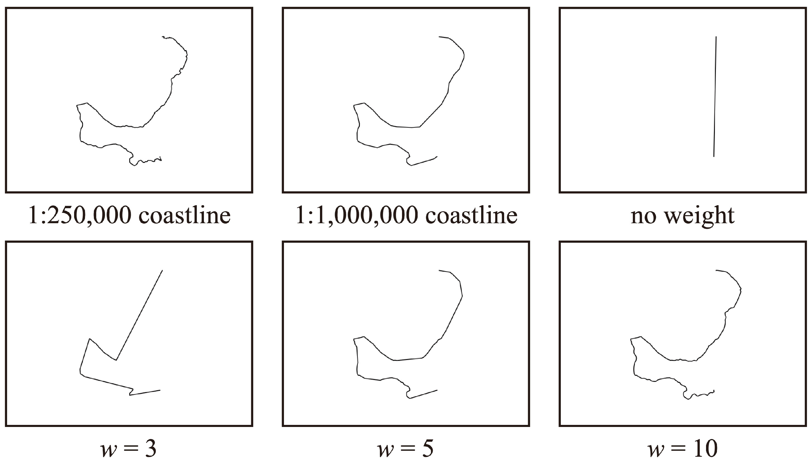
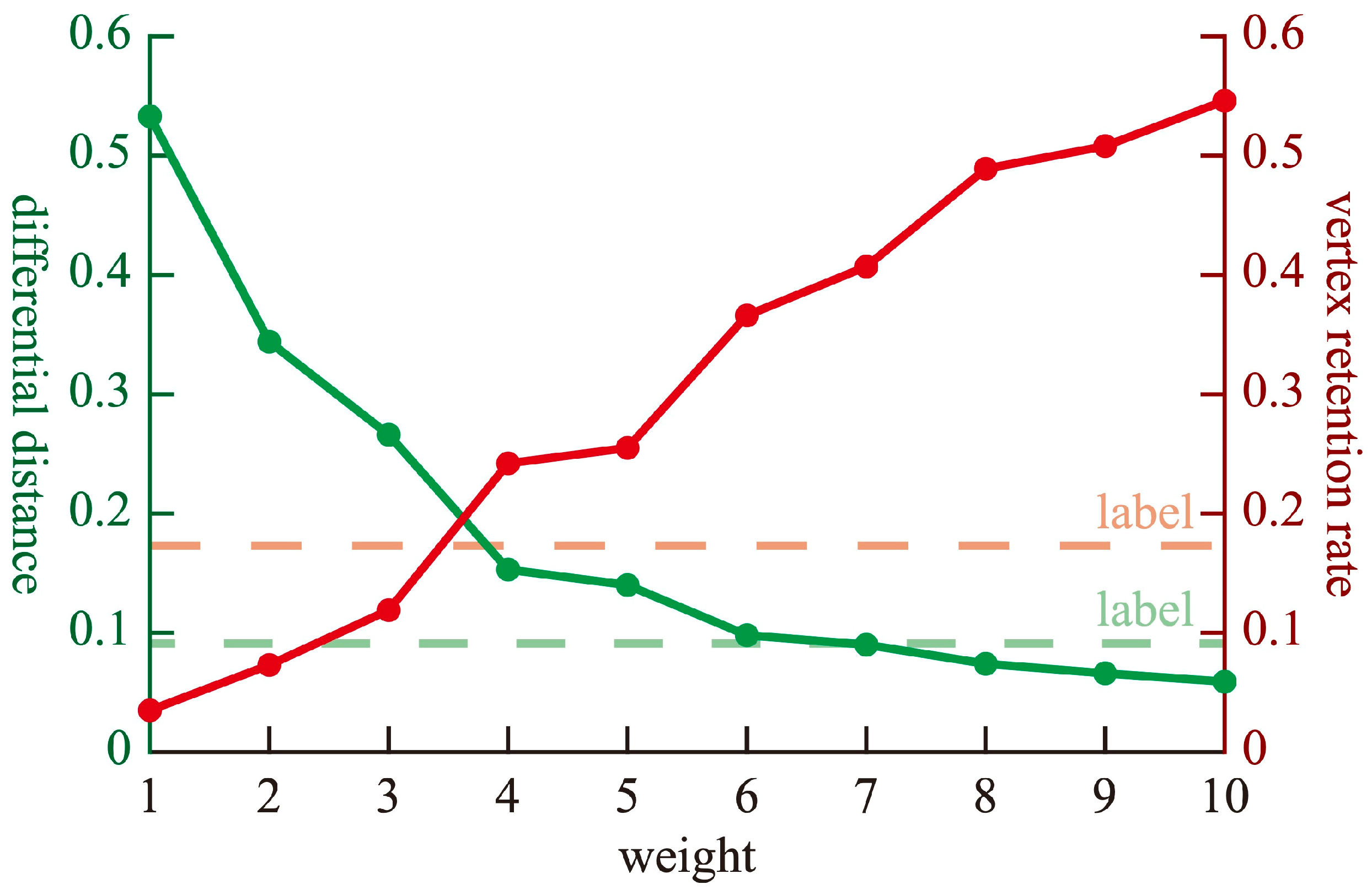
5.1. Parameter Discussion
5.2. Comparison with Existing Methods
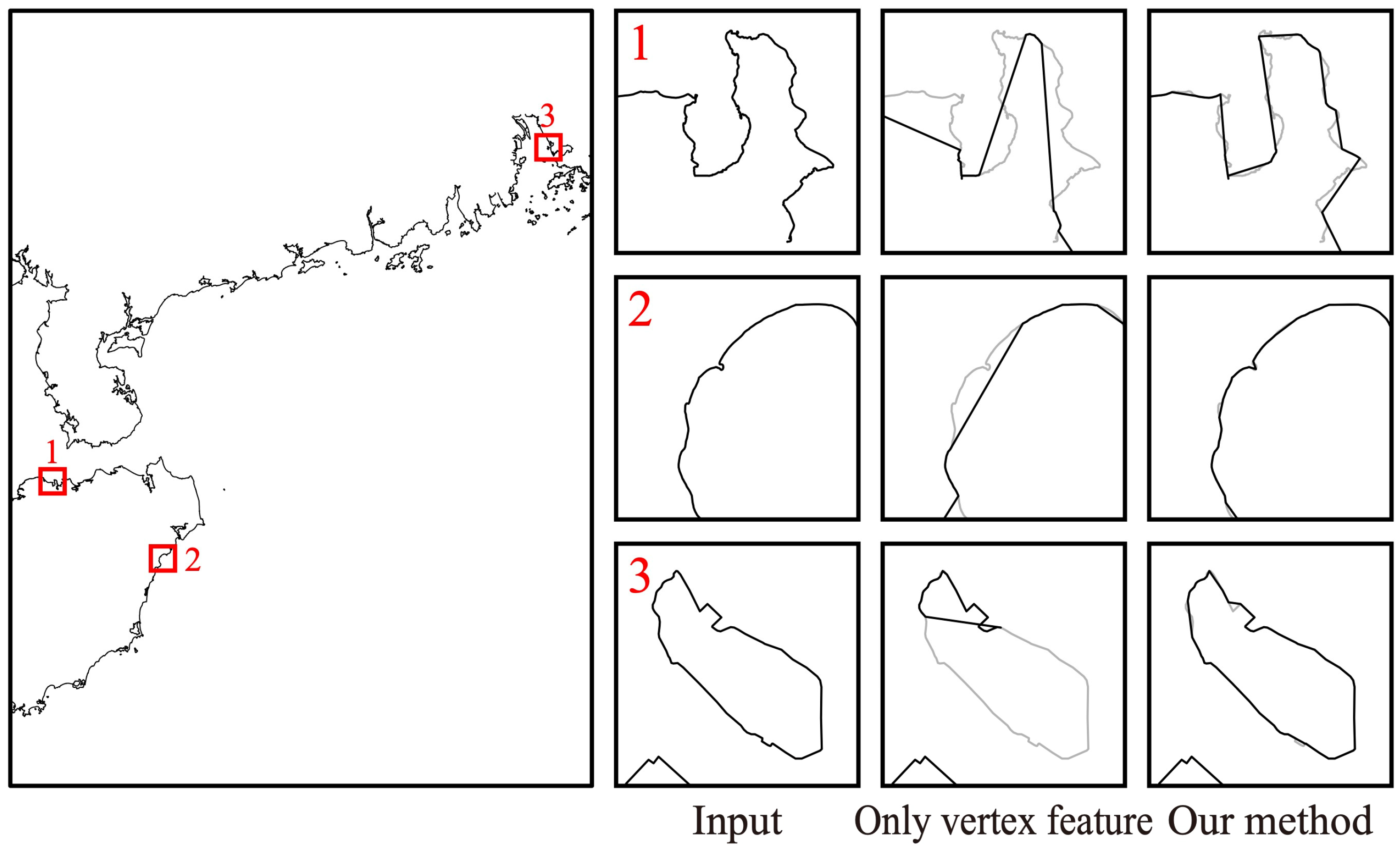
5.3. Ablation Experiment for Integrating Edge Features
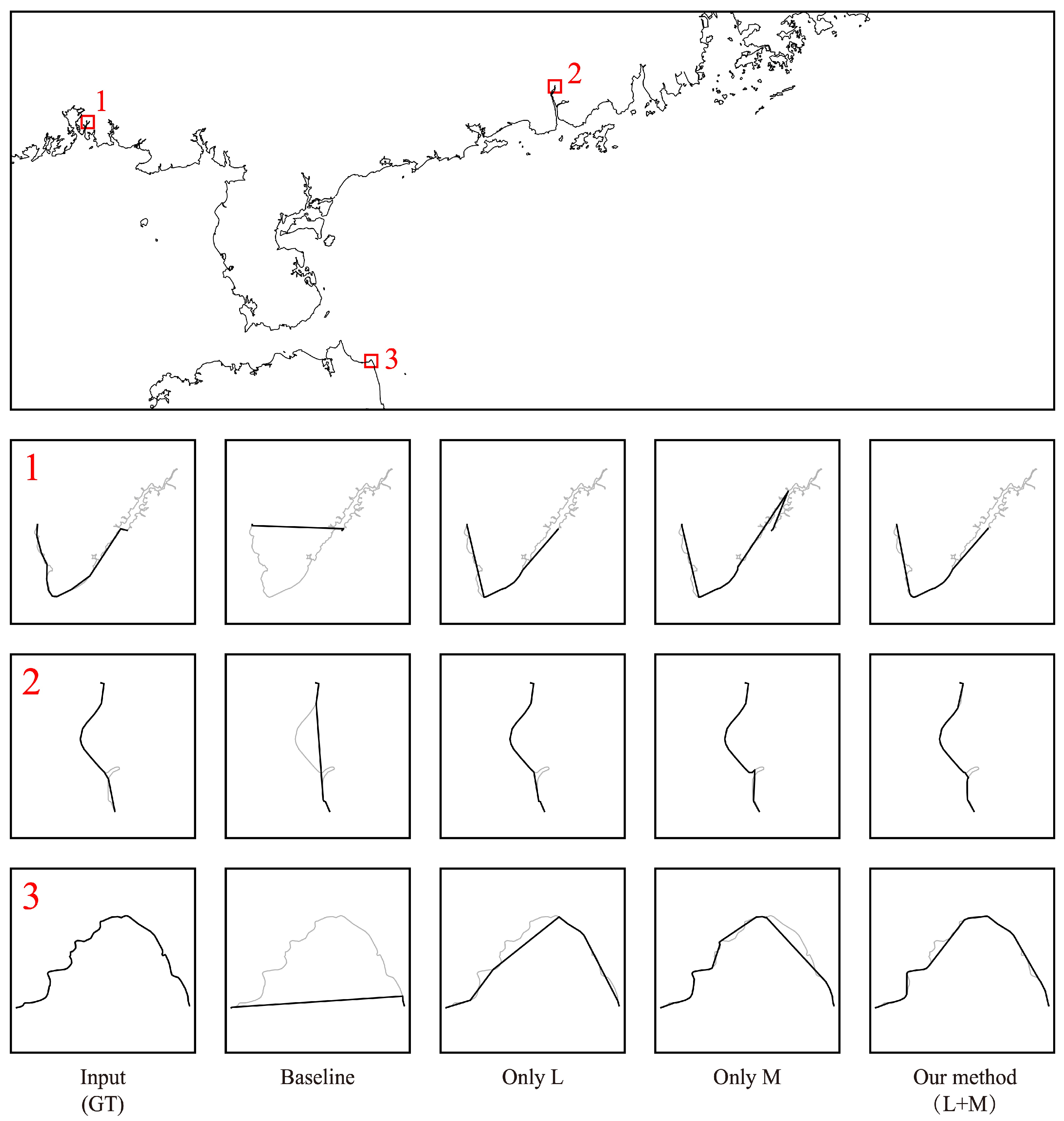
5.4. Ablation Experiment for the Architecture for Retaining Crucial Geographic Features
6. Conclusions
Author Contributions
Funding
Data Availability Statement
Acknowledgments
Conflicts of Interest
References
- Yin, H.M. A generalization of geographic conditions maps constrained by both spatial and semantic scales. Acta Geod. Cartogr. Sin. 2021, 50, 426. [Google Scholar]
- Lan, Q.P. Research on Multi-Scale Concatenated Update Methods for Map Data. Ph.D. thesis, Wuhan University, Wuhan, China, 2010. [Google Scholar]
- Shen, Y.L. Simplified Representation of Map Elements from Computer Vision Perspective. Ph.D. thesis, Wuhan University, Wuhan, China, 2019. [Google Scholar]
- Du, J.W.; Wu, F.; Xing, R.X.; Gong, X.R.; Yu, L.Y. Segmentation and sampling method for complex polyline generalization based on a generative adversarial network. Geocarto Int. 2021, 37, 4158–4180. [Google Scholar] [CrossRef]
- Wu, F.; Gong, X.Y.; Du, J.W. Overview of the Research Progress in Automated Map Generalization. Acta Geod. Cartogr. Sin. 2017, 46, 1645–1664. [Google Scholar]
- Li, J.; Ma, J.S.; Shen, J.; Yang, M.M.; Liu, L. Improvements of linear features simplification algorithm based on vertexes clustering. J. Geomat. Sci. Technol. 2013, 30, 525–529, 534. [Google Scholar]
- Douglas, D.H.; Peucker, T.K. Algorithms for the reduction of the number of points required to represent a digitized line or its caricature. Cartogr. Int. J. Geogr. Inf. Geovis. 1973, 10, 112–122. [Google Scholar] [CrossRef]
- Amiraghdam, A.; Diehl, A.; Pajarola, R. LOCALIS: Locally-adaptive Line Simplification for GPU-based Geographic Vector Data Visualization. Comput. Graph. Forum 2020, 39, 443–453. [Google Scholar] [CrossRef]
- Liu, B.; Liu, X.C.; Li, D.J.; Shi, Y.T.; Fernandez, G.; Wang, Y.D. A Vector Line Simplification Algorithm Based on the Douglas-Peucker Algorithm, Monotonic Chains and Dichotomy. ISPRS Int. J. Geo-Inf. 2020, 9, 251. [Google Scholar] [CrossRef]
- Wu, F.; Deng, H.Y. Using Genetic Algorithms for Solving Problems in Automated Line Simplification. Acta Geod. Cartogr. Sin. 2003, 32, 349–355. [Google Scholar]
- Jiang, B.; Nakos, B. Line Simplification Using Self-Organizing Maps. In Proceedings of the ISPRS Workshop on Spatial Analysis and Decision Making, Hong Kong, China, 3–5 December 2003. [Google Scholar]
- Yu, B.; Yin, H.T.; Zhu, Z.X. Spatio-Temporal Graph Convolutional Networks: A Deep Learning Framework for Traffic Forecasting. In Proceedings of the Twenty-Seventh International Joint Conference on Artificial Intelligence, Stockholm, Sweden, 13–19 July 2018; pp. 3634–3640. [Google Scholar]
- Yan, X.F.; Ai, T.H.; Yang, M.; Yin, H.M. A graph convolutional neural network for classification of building patterns using spatial vector data. ISPRS J. Photogramm. Remote Sens. 2019, 150, 259–273. [Google Scholar] [CrossRef]
- Zheng, C.Y.; Guo, Q.S.; Hu, H.K. The Simplification Model of Linear Objects Based on Ant Colony Optimization Algorithm. Acta Geod. Cartogr. Sin. 2011, 40, 635–638. [Google Scholar]
- Duan, P.X.; Qian, H.Z.; He, H.W.; Xie, L.M.; Luo, D.H. A Line Simplification Method Based on Support Vector Machine. Geomat. Inf. Sci. Wuhan Univ. 2020, 45, 744–752. [Google Scholar]
- Cheng, B.; Liu, Q.; Li, X.; Wang, Y. Building simplification using backpropagation neural networks: A combination of cartographers’ expertise and raster-based local perception. GISci. Remote Sens. 2013, 50, 527–542. [Google Scholar] [CrossRef]
- Zhang, Q.N.; Liao, K. Line Generalization Based on Structure Analysis. Acta Sci. Nat. Univ. Sunyatseni 2001, 40, 118–121. [Google Scholar]
- Qian, H.Z.; Wu, F.; Chen, B.; Zhang, J.H.; Wang, J.Y. Simplifying Line with Oblique Dividing Curve Method. Acta Geod. Cartogr. Sin. 2007, 36, 443–449+456. [Google Scholar]
- Visvalingam, M.; Whyatt, J.D. Line generalisation by repeated elimination of points. Cartogr. J. 1993, 30, 46–51. [Google Scholar] [CrossRef]
- Li, Z.L.; Openshaw, S. Algorithms for the Automated Line Generalization Based on Natural Principle of Objective Generalization. Int. J. Geogr. Inf. Syst. 1992, 6, 373–389. [Google Scholar] [CrossRef]
- Nakos, B.; Mitropoulos, V. Critical Points Detection Using the Length Ratio (LR) for Line Generalization. Cartographica 2003, 40, 35–51. [Google Scholar] [CrossRef]
- Teh, C.H.; Chin, R.T. On the Detection of Dominant Points on Digital Curves. IEEE Trans. Pattern Anal. Mach. Intell. 1989, 11, 859–872. [Google Scholar] [CrossRef]
- Chrobak, T.A. Numerical Method for Generalizing the Linear Elements of Large-Scale Maps, Based on the Example of Rivers. Cartogr. Int. J. Geogr. Inf. Geovis. 2000, 37, 49–56. [Google Scholar] [CrossRef]
- Zhu, K.P.; Wu, F.; Wang, H.L.; Zhu, Q. Improvement and Assessment of Li-Openshaw Algorithm. Acta Geod. Cartogr. Sin. 2007, 36, 450–456. [Google Scholar]
- Liu, H.M.; Fan, Z.D.; Xu, Z.; Deng, M. An Improved Local Length Ratio Method for Curve Simplification and Its Evaluation. Geogr. Geo-Inf. Sci. 2011, 27, 45–48. [Google Scholar]
- Deng, M.; Chen, J.; Li, Z.L.; Xu, Z. An Improved Local Measure Method for the Importance of Vertices in Curve Simplification. Geogr. Geo-Inf. Sci. 2009, 25, 40–43. [Google Scholar]
- Shen, Y.L.; Ai, T.H.; He, Y.K. A new approach to line simplification based on image processing: A case study of water area boundaries. ISPRS Int. J. Geo-Inf. 2018, 7, 41. [Google Scholar] [CrossRef]
- Wang, Z.S.; Müller, J.-C. Line Generalization Based on Analysis of Shape Characteristics. Cartogr. Geogr. Inf. Syst. 1998, 25, 3–15. [Google Scholar] [CrossRef]
- Li, J.H.; Wu, F.; Du, J.W.; Gong, X.Y.; Xing, R.X. Chart Depth Contour Simplification Based on Delaunay Triangulation. Geomat. Inf. Sci. Wuhan Univ. 2019, 44, 778–783. [Google Scholar]
- Ai, T.H.; Guo, R.Z.; Li, Y.L. A Binary Tree Representation of Curve Hierarchical Structure in Depth. Acta Geod. Cartogr. Sin. 2001, 30, 343–348. [Google Scholar]
- Huang, B.H.; Wu, F.; Zhai, R.J.; Gong, X.Y.; Li, J.H. The Line Feature Simplification Algorithm Preserving Curve Bend Feature. J. Geomat. Sci. Technol. 2014, 31, 533–537. [Google Scholar]
- Qian, H.Z.; He, H.W.; Wang, X.; Hu, H.M.; Liu, C. Line Feature Simplification Method Based on Bend Group Division. Geomat. Inf. Sci. Wuhan Univ. 2017, 42, 1096–1103. [Google Scholar]
- Ma, L. Features extraction of buildings and generalization using deep learning. In Proceedings of the 28th International Cartographic Conference, Washington, DC, USA, 2–7 July 2017. [Google Scholar]
- Kang, Y.; Gao, S.; Roth, R.E. Transferring multiscale map styles using generative adversarial networks. Int. J. Cartogr. 2019, 5, 115–141. [Google Scholar] [CrossRef]
- Courtial, A.; Ayedi, A.; Touya, G.; Zhang, X. Exploring the potential of deep learning segmentation for mountain roads generalisation. ISPRS Int. J. Geo-Inf. 2020, 9, 338. [Google Scholar] [CrossRef]
- Jiang, B.D.; Xu, S.F.; Li, Z.W. Polyline simplification using a region proposal network integrating raster and vector features. GISci. Remote Sens. 2023, 60, 2275427. [Google Scholar] [CrossRef]
- Yu, W.H.; Chen, Y.X. Data-driven polyline simplification using a stacked autoencoder-based deep neural network. Trans. GIS 2022, 26, 2302–2325. [Google Scholar] [CrossRef]
- Du, J.W.; Wu, F.; Zhu, L.; Liu, C.Y.; Wang, A.D. An ensemble learning simplification approach based on multiple machine-learning algorithms with the fusion using of raster and vector data and a use case of coastline simplification. Acta Geod. Cartogr. Sin. 2022, 51, 373–387. [Google Scholar]
- Guo, X.; Liu, J.N.; Wu, F.; Qian, H.Z. A Method for Intelligent Road Network Selection Based on Graph Neural Network. Data 2022, 7, 10. [Google Scholar] [CrossRef]
- Buffelli, D.; Vandin, F. The Impact of Global Structural Information in Graph Neural Networks Applications. ISPRS Int. J. Geo-Inf. 2023, 12, 336. [Google Scholar] [CrossRef]
- Defferrard, M.; Bresson, X.; Vandergheynst, P. Convolutional neural networks on graphs with fast localized spectral filtering. In Proceedings of the 30th International Conference on Neural Information Processing Systems, Barcelona, Spain, 5–10 December 2016. [Google Scholar]
- Raposo, P. Scale-specific automated line simplification by vertex clustering on a hexagonal tessellation. Cartogr. Geogr. Inf. Sci. 2013, 40, 427–443. [Google Scholar] [CrossRef]


| Method | Vertex Retention Rate | Differential Distance | Hausdorff Distance | Fréchet Distance |
|---|---|---|---|---|
| D–P | 0.23 | 0.11 | 1.08 | 1.11 |
| Hexagon clustering | 0.19 | 0.11 | 1.15 | 1.17 |
| Ternary bend groups | 0.24 | 0.10 | 1.12 | 1.14 |
| SVM | 0.23 | 0.26 | 1.59 | 1.61 |
| Our method | 0.26 | 0.18 | 1.36 | 1.39 |
| Method | Vertex Retention Rate | Differential Distance | Hausdorff Distance | Fréchet Distance |
|---|---|---|---|---|
| Only vertex feature | 0.24 | 1.06 | 3.65 | 3.68 |
| Our method | 0.26 | 0.18 | 1.36 | 1.39 |
| Method | Vertex Retention Rate | Differential Distance | Hausdorff Distance | Fréchet Distance |
|---|---|---|---|---|
| Baseline | 0.10 | 0.83 | 4.16 | 4.17 |
| Only L | 0.23 | 0.25 | 1.68 | 1.72 |
| Only M | 0.27 | 0.20 | 1.49 | 1.52 |
| Our method (M + L) | 0.26 | 0.18 | 1.36 | 1.39 |
Disclaimer/Publisher’s Note: The statements, opinions and data contained in all publications are solely those of the individual author(s) and contributor(s) and not of MDPI and/or the editor(s). MDPI and/or the editor(s) disclaim responsibility for any injury to people or property resulting from any ideas, methods, instructions or products referred to in the content. |
© 2025 by the authors. Published by MDPI on behalf of the International Society for Photogrammetry and Remote Sensing. Licensee MDPI, Basel, Switzerland. This article is an open access article distributed under the terms and conditions of the Creative Commons Attribution (CC BY) license (https://creativecommons.org/licenses/by/4.0/).
Share and Cite
Chen, S.; Hu, A.; Xu, Y.; Wang, H.; Xie, Z. VE-GCN: A Geography-Aware Approach for Polyline Simplification in Cartographic Generalization. ISPRS Int. J. Geo-Inf. 2025, 14, 64. https://doi.org/10.3390/ijgi14020064
Chen S, Hu A, Xu Y, Wang H, Xie Z. VE-GCN: A Geography-Aware Approach for Polyline Simplification in Cartographic Generalization. ISPRS International Journal of Geo-Information. 2025; 14(2):64. https://doi.org/10.3390/ijgi14020064
Chicago/Turabian StyleChen, Siqiong, Anna Hu, Yongyang Xu, Haitao Wang, and Zhong Xie. 2025. "VE-GCN: A Geography-Aware Approach for Polyline Simplification in Cartographic Generalization" ISPRS International Journal of Geo-Information 14, no. 2: 64. https://doi.org/10.3390/ijgi14020064
APA StyleChen, S., Hu, A., Xu, Y., Wang, H., & Xie, Z. (2025). VE-GCN: A Geography-Aware Approach for Polyline Simplification in Cartographic Generalization. ISPRS International Journal of Geo-Information, 14(2), 64. https://doi.org/10.3390/ijgi14020064