Abstract
The Traveling Salesman Problem (TSP) is a classical discrete combinatorial optimization problem that is widely applied in various domains, including robotics, transportation, networking, etc. Although existing studies have provided extensive discussions of the TSP, the issues of improving convergence and optimization capability are still open. In this study, we aim to address this issue by proposing a new algorithm named IDINFO (Improved version of the discretized INFO). The proposed IDINFO is an extension of the INFO (weighted mean of vectors) algorithm in discrete space with optimized searching strategies. It applies the multi-strategy search and a threshold-based 2-opt and 3-opt local search to improve the local searching ability and avoid the issue of local optima of the discretized INFO. We use the TSPLIB library to estimate the performance of the IDINFO for the TSP. Our algorithm outperforms the existing representative algorithms (e.g., PSM, GWO, DSMO, DJAYA, AGA, CNO_PSO, Neural-3-OPT, and LIH) when tested against multiple benchmark sets. Its effectiveness was also verified in the real world in solving the TSP in short-distance delivery.
1. Introduction
The Traveling Salesman Problem (TSP) is a classic combinatorial optimization problem that seeks the shortest possible route for a salesman to visit a set of cities exactly once and return to the origin city. As one of the most intensively studied problems in operations research and computer science, the TSP has profound implications across multiple domains, including logistics planning, integrated circuit design, and robotics [1,2]. In the field of geospatial science, the TSP has been widely applied to optimize logistics distribution, tourism route planning, navigation systems, and urban traffic management [3,4,5]. For instance, in urban scenarios, the TSP can be used to determine the shortest delivery routes for couriers, significantly reducing transportation costs and improving efficiency [6]. Moreover, with the integration of GIS technologies, TSP algorithms can leverage geospatial data, such as road networks and point-of-interest locations, to generate more accurate and practical routing solutions.
Mathematically, the TSP can be represented as a graph where cities correspond to nodes, and the travel distances between them correspond to weighted edges. The objective is to determine the Hamiltonian cycle with the minimum total weight. The optimization for the TSP has an NP-complete computational complexity, which was discussed in a massive number of studies [7,8]. According to the existing work, optimizations for the TSP can be classified as classic methods, artificial intelligence-based algorithms, and metaheuristic algorithms. Classic methods, e.g., Enumeration, Integer Programming (IP), Nearest Neighbor (NN), etc., are effective but suffer in terms of time and computing costs. The second kind of algorithm is proposed to solve the approximate solution of the TSP based on artificial intelligence, such as deep reinforcement learning (DRL) [9,10,11]. For small-scale instances, artificial intelligence-based methods are competitive. However, they struggle with medium and large instances due to significant computational costs and time overhead, which also create an opportunity for the metaheuristic algorithms. Metaheuristic algorithms have been particularly effective in solving large-scale TSP instances in geospatial applications, such as optimizing delivery routes in urban areas or planning tourist itineraries based on real-world geographic data. In the last two decades, metaheuristic algorithms have provided practical solutions for the TSP, whether small, medium, or large instances. They aimed to achieve approximate or optimal solutions within the actual execution time of the optimization problem with the advantages of low computational effort and high optimization efficiency. Most current metaheuristic algorithms are derived from Swarm Intelligence (SI) algorithms such as PSO (Particle Swarm Optimization) and SSA (Sparrow Search Algorithm) algorithms [12,13], which are limited in convergence efficiency and local optimum.
In this study, we propose a new metaheuristic algorithm, IDINFO, for the symmetric TSP based on the INFO (weighted mean of vectors) algorithm. The INFO algorithm is a physics-based metaheuristic algorithm that applies the weighted mean method to solid structures and updates the position of vectors through three core stages [14]. Compared with the existing metaheuristic algorithms and their improvement methods, e.g., GA, PSO, GWO, and SCA, it excels in both exploration and exploitation, showcasing superior performance and fast convergence time. The proposed IDINFO is an extension of the INFO algorithm in discrete space with optimized searching strategies. IDINFO applies a multi-strategy search and a threshold-based 2-opt and 3-opt local search to improve the local searching ability and avoid the issue of local optima. Moreover, IDINFO demonstrates its potential in solving real-world routing problems, such as optimizing delivery routes in urban road networks. We use the TSPLIB library to estimate the performance of the IDINFO. Our algorithm outperforms the existing representative algorithms (e.g., PSM, GWO, DSMO, CNO_PSO, Neural-3-OPT, and LIH) when tested against multiple benchmark sets. Additionally, we verify its effectiveness in solving the TSP in short-distance delivery. The contributions of this study are as follows:
- A discrete version of INFO was proposed to accomplish the challenges of applying INFO to the TSP by encoding the relevant variables and introducing several new operators;
- To address the low accuracy and efficiency in the discrete version of INFO, we improve its searching strategies by using a multi-strategy and threshold-based 2-opt and 3-opt local searching.
The remainder of this paper is organized as follows. Section 2 reviews the related work on the TSP, including classic methods, artificial intelligence-based algorithms, and metaheuristic algorithms. Section 3 introduces the proposed IDINFO algorithm, detailing its discrete encoding, operator definitions, and improved search strategies. Section 4 presents the experimental results, including parameter sensitivity analysis, performance evaluation on TSPLIB instances, and a real-world case study of short-distance delivery. Section 5 concludes the paper by summarizing the contributions, discussing limitations, and outlining future research directions.
2. Related Work
This section reviews the related work in solving the TSP using classic methods, artificial intelligence-based algorithms, and metaheuristic algorithms, respectively.
Classic Methods: Based on the previous work, classic methods include two types: exact algorithms and approximation algorithms. Exact algorithms, such as Branch and Bound (BnB) and Dynamic Programming (DP), have been widely utilized to find the optimal solution for the TSP. The variants of exact algorithms [15], such as Concorde and Gurobi, are noteworthy examples of exact TSP solvers [16]. Nevertheless, the computation time and cost of exact algorithms grow exponentially as the problem scale increases, thereby rendering it difficult to obtain optimal solutions within a limited computation time. Based on the existing study, the exact algorithms are not easy to calculate when the number of nodes exceeds 40 [17]. As a result, approximation algorithms, such as the Nearest Neighbor (NN) and Christofides algorithm [18], have emerged as an alternative, offering quality-assured approximate solutions in polynomial time [19]. In the minimization problem, the approximate solution obtained by the approximation algorithm in the worst case does not exceed a certain multiple of the optimal solution. This kind of method has certain application significance but loses some accuracy of TSP optimization.
Artificial intelligence-based algorithms: In the last decades, artificial intelligence-based algorithms for the TSP have demonstrated remarkable decision-making and learning capabilities. For example, Vinyals et al. [11] proposed the well-known Pointer Networks model, which successfully learned the approximate solutions of the TSP and performed well at around 20 nodes. Bello et al. [9] proposed a Neural Combinatorial Optimization (NCO) framework by integrating neural networks with DRL (Deep Reinforcement Learning) techniques, delivering approximate solutions for TSP instances of around 100 nodes. Furthermore, by introducing the reinforcement learning training, Ma et al. [10] presented the Graph Pointer Networks (GPNs) to solve small-scale TSPs and demonstrated its potential for the medium and large TSP, albeit with a training time of up to 30 min for one iteration for an instance of 50 nodes. Based on convolutional neural networks combined with long and short-term memory, Sultana et al. [20] proposed a non-Euclidean TSP network (NETSP) using randomly generated simple instances to solve various common TSP instances. However, only approximate solutions can be obtained for more than 42 nodes based on their method. Luo et al. [21] illustrated a new graph convolutional encoder and multi-headed attention decoder network (GCE-MAD Net) to obtain the solution with a higher quality. However, their method is still limited to small-scale instances of the TSP. Although previous studies have demonstrated the importance of artificial intelligence-based techniques for solving small-scale TSPs, they are associated with significant computational costs and time overhead, thereby limiting its scalability to medium and large instances. Consequently, the current artificial intelligence-based methods for the TSP are not particularly competitive when compared with metaheuristic algorithms.
Metaheuristic Algorithms: The metaheuristic algorithms focus on determining the approximate or optimal solutions for the optimization problem. They simulate natural and human intelligence while combining the exploration of the search space with the exploitation of the region around the obtained solution. Based on the inspiration sources of metaheuristic algorithms, they can be classified as evolutionary algorithms, swarm intelligence algorithms, and physics-based algorithms [22,23]. Evolutionary-based algorithms are inspired by biological evolution, which encompasses a range of methods such as Genetic Algorithm (GA), Memetic Algorithm (MA), and Differential Evolution algorithm (DE) [24,25,26], etc. Swarm-based approaches reflect the patterns of cooperation observed in natural systems, such as Swallow Swarm Optimization (SSO) [27], Whale Optimization Algorithm (WOA) [28], Sparrow Search Algorithm (SSA) [13], etc. Taking Particle Swarm Optimization (PSO) as an example, its basic principle is that individuals change their search patterns by learning from their own and team’s experiences [12,29]. Beyond that, Ant Colony Optimization (ACO) exhibits intelligent behavior by means of communication and collaboration between individuals using pheromones [30,31]. Although these algorithms have been verified with satisfactory accuracy, exhibiting outstanding performance and low computational overhead, the issues of slow convergence speed and low accuracy are still open [32]. Physics-based algorithms are derived from the laws of physical phenomena [33]. For example, the simulated annealing algorithm (SA) was proposed based on the similarity between the process of annealing solids in physics and general optimization problems [34]. At present, the potential of physics-based metaheuristic algorithms in TSPs has been largely overlooked [35].
3. Methodology
From the perspective of graph theory, the input of the TSP is a complete graph with weighted edges. There are two kinds of TSP variants: a symmetric one and an asymmetric one. The symmetric TSP indicates the distance from city u to city v is the same as that from city v to city u. This process can be described as an input with an undirected graph. Conversely, the asymmetric TSP has inputs with directed graphs. In this paper, the proposed IDINFO is used to solve the symmetric TSP. Given a connected graph G = (V, E), where V = {v1, v2, …, vn} represents the set of vertices (cities) and E = {eij} (i, j ∈ V) represents the set of weighted edges. The solution of the TSP is to determine a Hamiltonian cycle with the shortest length. Let dij denote the distance between vertex vi and vj and a decision variable xij is introduced as Equation (1). The objective function of the TSP can be expressed as Equation (2).
The proposed IDINFO for the TSP is derived from the INFO algorithm which includes three core stages: updating rule, vector combining, and local search. Since the TSP belongs to a discrete optimization problem, INFO cannot be directly applied to solve it. We propose a discretized INFO (DINFO) method, which constructs discrete encoding and operators tailored for the TSP, enabling INFO to perform searches in a discrete space. However, as the problem scale increases, DINFO still exhibits certain limitations in search efficiency and solution quality. To further enhance performance, we optimize the search strategy based on DINFO and propose an improved version, IDINFO. This method enhances local search capability and refines the solution update mechanism, thereby improving convergence speed and global search ability.
3.1. Constructing the DINFO
For the TSP, the position x of a vector can be considered as a Hamiltonian path comprising all vertices, i.e., the position of each vector represents a solution. Let the position of the ith vector be expressed as xi = (vi1, vi2, …, vin), where vi1, vi2, …, vin denotes the number of vertices n. The solution is encoded through a traversal of the city sequence, which means starting from vi1, passing through vi2, …, vin, and finally returning to vi1. The DINFO is obtained based on the following definitions.
Definition 1.
Addition between position and permutation sequence: Let xi = (vi1, vi2, …, vin) denote the position of the vector and the swap operator SO (vi1, vi2) be introduced, where vi1 and vi2 denote two city nodes. If the operation xi + SO (vi1, vi2) is performed, the positions of vi1 and vi2 in the solution sequence xi are exchanged. The sequence SS = (SO1, SO2, …, SOn) comprising multiple swap operators is defined as a permutation sequence. Accordingly, xi + SS indicates that the swappers in the permutation sequence SS act on xi in turn, resulting in a new position xj, as shown in Equation (3). It is pertinent to note that swappers in different orders may produce dissimilar solution sequences.
Definition 2.
Addition between two permutation sequences: The addition of two sequences SS1 and SS2 leads to the formation of a new permutation sequence new_SS that encompasses all the swappers of both sequences, as shown in Equation (4).
Definition 3.
Subtraction between two positions: In contrast to the addition operation of Definition 1, the subtraction of two positions is a permutation sequence, as shown in Equation (5).
Definition 4.
Multiplication between random number and permutation sequence: In DINFO, the new permutation sequence can be obtained by multiplication between the random number r and the permutation sequence SS = (SO1, SO2, …, SOn), where n denotes the length of SS. According to the numerical distribution of r, the results of the multiplication operation can be categorized as follows:
If r ∈ [0, 1], the result of the multiplication is the filtration of the permutation sequence based on the probability r and the retention of a rounded value of r × n swappers. Therefore, the sequence is not retained when r is 0. Analogously, if r < 0, the operation of (−r) × SS can be executed following the above-mentioned steps, followed by the inversion of the sequence using the reverse operator Fliplr to obtain the new sequence.
Definition 5.
Addition between two positions: The second and third stages of the algorithm involve the process of combining different vectors by probability. This combination operation can be expressed as follows:
where μ, η ∈ [0, 1]. Consistent with the operation in Definition 4, we obtain two position sequences pi and pj after screening. However, the merging of two positions may result in the revisiting of certain cities, thereby violating coding regulations. Therefore, we define the Correction operator, which modifies solutions that do not conform to coding rules and restores them to a reasonable and correct range. Specifically, the Correction operator retains only the city numbers of their first appearance, eliminates any duplicate city visits, and subsequently assigns the unpreserved positions, using a random sequence of unvisited city numbers, to obtain the new positions.
3.2. Improvements of the DINFO
Although DINFO enables INFO to be applied to the TSP and demonstrates a certain level of solution capability, it still faces challenges in large-scale TSP instances due to high computational overhead and limited convergence performance. As the problem size increases, the redundancy in DINFO operations leads to a significant rise in computation time, while its original update strategy tends to become trapped in local optima in the later stages of the search, restricting further solution improvement. Moreover, as the complexity of the problem increases, the accuracy of DINFO solutions gradually declines, limiting its applicability.
To address these issues, we propose an improved version, IDINFO, which optimizes the search strategy to enhance computational efficiency and solution quality. Specifically, we refine the vector update mechanism to accelerate convergence, introduce adaptive 2-opt and 3-opt algorithms to strengthen local search capabilities and adopt an improved random perturbation strategy to enhance global exploration. The following sections will elaborate on IDINFO’s optimization strategies in terms of update rules, local search, and other aspects.
3.2.1. Optimization of Updating Rule
The updating rule stage of DINFO is the same as the original version of INFO, which consists primarily of two components: the mean-based method (MeanRule) and the convergence acceleration (CA), performing a global search in the space. MeanRule combines the weighted mean of two vector sets, namely a set of random differential vectors and a set of vectors comprising the current best, better, and worst solutions, to enhance exploration capabilities. Further details can be found in the literature [14]. The form of CA can be represented in Equation (8), utilizing vector xi to move the current vector xj in the search space, facilitating movement towards potentially better directions and improving the convergence speed. Here, f(x) denotes the objective function of the optimization problem, and randn represents a random value following a normal distribution. The updating rules stage results in the generation of two new vectors, and , as expressed in Equation (4). The parameter in Equation (9) denotes the lth vector in the gth iteration, representing the current vector with l being a member of the interval [1, NP]. NP refers to the total number of vectors. Parameters , and denote distinct random vectors, and xbs, xws, and xbt represent the best, worst, and better solutions, respectively, among all vectors in the population. xbt is randomly selected from the top five solutions. R indicates a normally distributed random value and σ is the vector scaling rate.
Although INFO possesses commendable performance capabilities, its fundamental principles give rise to unavoidable drawbacks in the form of high computational efforts and significant time overheads. In this study, we optimized the convergence acceleration CA of INFO, which is shown in Equation (10).
where f(x) is the objective function. It represents the total distance length of the city sequence traversing x in the algorithm to solve the TSP with a large value resulting in R assuming a very small value in most cases. In accordance with Definition 4, when the random number takes a very small value, the permutation sequence retention length approaches 0, which means that the CA increases the computational effort, but hardly works. To mitigate this computational burden, without impinging on performance, we optimize the first stage of the algorithm by rounding off CA, thereby reducing running times and improving algorithmic speed.
3.2.2. Multi-Strategy Local Search
The process of vector combining in DINFO is also the same as INFO, which involves the merging of vectors , , and the current vector . However, the space around is not fully explored during this process. To address this limitation and improve the local search capability in the second stage, we propose a multi-strategy local search method. This method employs three simple and commonly used search operators, namely exchange, invert, and relocate, as shown in Equation (11), where r represents a random number. The resulting vector generated by this exploration is denoted as . Given that the invert operation alters the connections of only two chains, whereas the exchange and relocate operators modify a greater number of chains, it is evident that they introduce more substantial local adjustments, thereby increasing the likelihood of discovering superior outcomes during the search process. Consequently, the probabilities associated with three operations are unequal, with values assigned as, for instance, 0.4, 0.2, and 0.4. To optimize efficiency, only one operation occurs at a time, and the probability reflects the percentage of times each operation is performed.
Figure 1 indicates a detailed illustration of the specific operations involved in the search process using five nodes. The exchange operator, which is based on the sequence length of the vector, generates two random numbers as the position indexes of the two nodes and swaps the nodes in the two positions. The invert operator, on the other hand, reverses the subsequence between two random positions. Similarly, the relocate operator inserts the node in the first position behind the node in the second position. Finally, the fitness values of the new vectors and are compared, and a decision is made on whether to keep or drop .
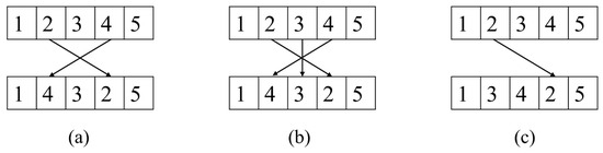
Figure 1.
Illustration of operators, (a) exchange operator, (b) invert operator, (c) relocate operator.
3.2.3. Local Search Improvement
The same as for INFO, the local search stage of DINFO is used to prevent the algorithm from succumbing to local optima. In the local search stage, MeanRule and the global best position xbs are used to promote the exploitation and search for the convergence of the global optimal. During this process, a novel vector can be produced around xbs, as shown in Equation (12). Additionally, a new solution xrnd is proposed, calculated as described by Equations (13) and (14). This involves combining the average solutions xavg of random vector groups xa, xb, xc, along with xbs and xbt, to facilitate a better search of the solution space. In the following equations, rand and Φ denote random numbers from the range [0, 1], v1 and v2 are constants that can increase the influence of xbs on .
In the above stage, INFO fuses together the average of three random differential vectors, the current best and the better solution in proportion to obtain xrnd to facilitate the mining of the optimal solution. This procedure is easy to operate and effective in scenarios with real spaces, such as continuous optimization functions. But for the TSP, it is difficult to perfectly fuse the five vectors together while sustaining the advantages of their respective solutions. More often, the vectors resulting from the fusion are not well associated with them. Moreover, this stage does not sufficiently deter the algorithm from succumbing to local optima. So, we propose an approach to replace the vector fusion operation by utilizing a threshold-based 2-opt local search on the current globally optimal solution. The 2-opt algorithm, originally introduced by Croes for solving the TSP, has been widely adopted for path-planning tasks [36]. The fundamental concept of this algorithm is to randomly select two links, remove them from the original route, and reconnect the remaining segments iteratively to improve the overall path until no better solution can be found. Therefore, in this paper, the computation of xrnd is improved as follows:
where Thd is the threshold. If a better solution cannot be found after multiple attempts and the cumulative number of attempts reaches the threshold, the 2-opt algorithm terminates the search. It has a time complexity of O(n2), which increases with repeated calls and iterations. By setting a threshold, 2-opt can avoid becoming stuck in an invalid search for an extended period, thereby reducing complexity and significantly shortening search time.
Apart from that, this paper proposes a threshold-based 3-opt local search approach for the new vector to a deep search to further enhance the algorithm’s ability to avoid local optima, as presented in Equation (16). Unlike the 2-opt method, the 3-opt algorithm randomly eliminates three non-adjacent links and offers seven distinct reconnection techniques to link the remaining segments [37]. The optimal reconnection type is determined through comparison, whereas the 2-opt only has one connection method. Previous research has demonstrated that the 3-opt approach is more efficient and effective than the 2-opt in identifying the optimal solution [38]. The time complexity of the 3-opt algorithm is O(n3). Similarly, the setting of the threshold Thd can enable the 3-opt to improve the ability of the IDINFO algorithm to find the optimal solution and improve the solution accuracy while reducing the time consumption caused by invalid local search.
4. Experiments and Discussions
In this section, we thoroughly validate the performance of the proposed IDINFO algorithm. Firstly, we discuss the influence of the algorithm parameters on performance. Then, we use instances from the TSPLIB standard test library as well as automatically generated instances to validate the efficacy of IDINFO. We showcase its performance across datasets of varying sizes, city distributions, and distance metrics. Additionally, we provide a detailed comparison between our proposed algorithm and other metaheuristic and artificial intelligence-based methods. Finally, we present two application case studies under different scenarios.
In the results, the number in the instance name indicates the number of cities. For example, the TSPLIB instance ulysses16 corresponds to a real-world dataset with 16 cities. These instances are primarily derived from real-world applications, with each city represented by a coordinate. Each city in the dataset is depicted as a coordinate point. The distance matrix is either computed based on Euclidean distances derived from the coordinates or directly obtained from the TSPLIB dataset. This matrix plays a critical role in calculating the total route length, which is the optimization target in the TSP. Any optimization method in the experiment considers the total route length as the fitness value in the TSP, where the minimum route length is assumed to be the optimal solution. The objective function of the TSP is to find the shortest route.
Additionally, any instances named as “TSP” indicate that the cities are automatically generated, and the number following represents the number of cities. Unlike the TSPLIB instances, the distance metric for these random instances is based on Manhattan distances rather than Euclidean distances. This variation is intended to test the algorithm’s ability to handle different types of distance metrics.
All experiments are conducted on a computer with 16.0 GB of RAM and a 2.10 GHz processor, using MATLAB 2016b on the Windows 10 operating system.
4.1. Effectiveness Verification
To verify the best performance of IDINFO, the algorithm parameters need to be determined. We discuss the method of parameter selection to prove the feasibility and effectiveness of the algorithm. In addition, we examine the performance of IDINF on datasets with different characteristics, estimating the ability of IDINFO with different measures of the number of cities, city distribution, and distance metrics.
4.1.1. Parameters Analysis
To demonstrate the effectiveness of the IDINFO, 18 classical examples from the TSP standard library [39] are selected in the experiments with the number of cities varying from 14 to 76. Meanwhile, we analyze the impact of two important parameters, i.e., the number of vectors and the number of iterations, on the performance of DINFO and the IDINFO and evaluate the algorithm’s stability based on the standard deviation (Std). Using the typical eil51 dataset as an example, the experimental results are averaged over 10 runs. Table 1 and Figure 2 present the effect of different population sizes (10–200) on the stability of DINFO and IDINFO under a fixed maximum iteration count of 1000. The experimental results show that when the population size is small (e.g., 10 and 50), the optimization performance is poor, and the results fluctuate significantly. The standard deviations for DINFO and IDINFO are 1.634/1.455 (population size = 10) and 1.353/1.212 (population size = 50), indicating unstable convergence. As the population size increases, the optimization performance improves, and fluctuations decrease. When the population size reaches 100 or more, the standard deviation stabilizes at 0.951 for DINFO and 0.889 for IDINFO.

Table 1.
Influence of vector population size on DINFO and IDINFO.
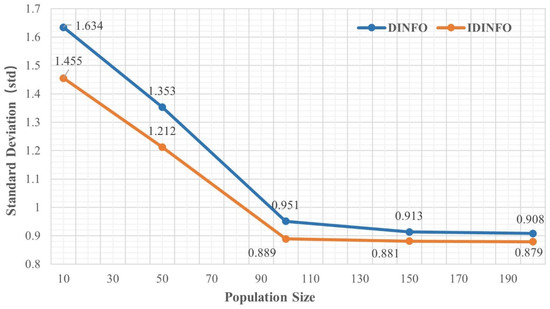
Figure 2.
Standard deviation under different population sizes.
Similarly, Table 2 and Figure 3 illustrate the effect of different iteration counts (100–2000) on optimization performance when the population size is fixed at 100. The results indicate that with fewer iterations (e.g., 100 and 500), the optimization performance is poor, and the standard deviation is high (DINFO: 1.844 and 1.379; IDINFO: 1.532 and 1.221), showing that the algorithm has not yet converged. As the number of iterations increases, the optimization results improve, and the standard deviation gradually decreases. When the iteration count reaches 1000 or more, the standard deviations for DINFO and IDINFO stabilize at 0.958 and 0.832, respectively, indicating convergence.
Table 2.
Influence of total iteration on DINFO and IDINFO.
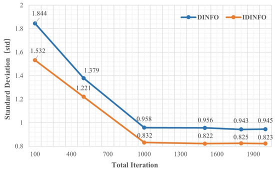
Figure 3.
Standard deviation under different iteration counts.
Overall, setting the number of vectors to ≥100 and the iteration count to ≥1000 effectively ensures both optimization performance and result stability. Therefore, we adopt this parameter configuration in subsequent experiments to balance performance and computational cost.
We introduce the threshold-based 2-opt and 3-opt local search algorithms to the IDINFO. The size of the threshold affects the search capability of the IDINFO.
To confirm the threshold properly, we adjust its value and analyze IDINFO’s optimization effectiveness and convergence time. In the tests, both 2-opt and 3-opt share the same threshold setting. In this testing, thresholds of the 2-opt and 3-opt local search algorithms are set the same. We summarize the average results from 10 runs to evaluate the effect of the threshold on the average route length (Average Solution) and convergence time (Convergence Time), as shown in Figure 4. The blue line represents the Average Solution, while the red line represents the Convergence Time. From Figure 4, it is observed that as the threshold increases, the route length gradually improves and reaches 433.06 at a threshold of 20, indicating that increasing the threshold enhances search quality. However, when the threshold further increases to 30 and 40, the improvement becomes negligible (432.56 and 432.38, respectively), suggesting that an excessively high threshold does not significantly enhance performance. On the other hand, the convergence time increases significantly with a higher threshold. It grows from 23.62 s at a threshold of 5 to 29.21 s, 36.98 s, 60.47 s, and 84.77 s at thresholds of 10, 20, 30, and 40, respectively. Particularly, when the threshold exceeds 20, the computational cost rises sharply while the optimization gain saturates.
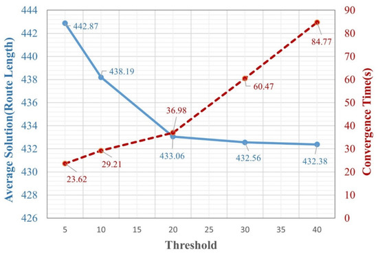
Figure 4.
The Influence of Threshold on 2-opt and 3-opt in IDINFO.
Considering both optimization performance and computational cost, we set the threshold for 2-opt and 3-opt local search to 20 in subsequent experiments to balance search efficiency and computational overhead.
4.1.2. Performance Estimation for the IDINFO
In this section, we first select 18 small-scale datasets (with fewer than 100 cities) and 11 medium-scale datasets (with 100 to 200 cities) from the TSPLIB to validate indicators such as solution accuracy and speed. As a classic dataset, TSPLIB is widely recognized as a benchmark for TSP research and provides a basis for horizontal comparison of algorithm performance. The instances in TSPLIB not only vary in scale but also cover various city distribution patterns, such as uniform and clustered distributions. For example, the rat99 and eil76 datasets exhibit typical uniform distributions, while d198 and pr439 exhibit typical clustered distributions. Additionally, there are irregularly distributed datasets (such as stt70) and grid-based distributions (such as ts225).
Using 18 distinct data sets, we test the DINFO and IDINFO through 30 repeated operations. The minimum value obtained from this process is regarded as the optimal solution for DINFO and IDINFO. Table 3 documents the optimal solution (Best), the average solution (Average) (the mean of 30 experiments), and their respective deviation rates from the TSPLIB public optimal solution (Opt). Here, the deviation rate of the optimal solution (Best_DR) is calculated based on Equation (17). Table 3 highlights results that reach the TSPLIB public optimal solution, with such results being bolded. The variation process of the deviation ratio of the solution with the problem size is shown in Figure 5a, while Figure 5b demonstrates the variation of convergence time on TSP instances.
Table 3.
Comparison of DINFO and IDINFO on some TSP instances.
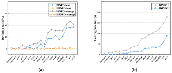
Figure 5.
Testing results of DINFO and IDINFO using TSP instances: (a) the deviation ratio of solutions on the TSP instances, (b) convergence time on the TSP instances.
In Table 3, DINFO reaches the optimal in five small instances, i.e., burma14, ulysses16, gr17, gr21, and ulysses22, which indicates that DINFO is effective in solving small TSP instances. In Figure 5a, we can find that the problem size scales up, and the deviation rate of the best solution of DINFO considerably increases, from 0.80% to 36.94%. Meanwhile, the deviation rate of the average solution is more obvious, from 0.28% to 46.61%, which indicates the susceptibility of DINFO to fall into local optima, thereby decreasing the accuracy of the solutions after the scale becomes larger. Similarly, the convergence time of DINFO is almost multiplied with the instance scale increasing, as shown in Figure 5b. In comparison, IDINFO achieved optimal solutions across all instances (see Table 3). The Average_DR of IDINFO on the first 10 instances is 0, indicating that it can accurately find the optimal solution in scenarios with no more than 31 city nodes. The average solution serves as a measure of the algorithm’s stability. Table 3 and Figure 5 reveal that all the average solution deviation rates of IDINFO are less than 1.65%, which is significantly smaller than DINFO. Although the introduction of 2-opt and 3-opt local search operations has relatively high time complexity, the performance of IDINFO consumes time level is still very low, as shown in Figure 5b. The convergence time of IDINFO is substantially shortened compared with DINFO. In most instances, we can obtain results within 60 s using IDINFO (see Figure 5b).
We also examine the capabilities of the IDINFO algorithm in solving larger-scale TSPs by selecting 12 instances from the TSPLIB library. The number of cities in these instances ranges from 76 to 200. The experimental results of 30 test statistics are presented in Table 4.
Table 4.
Results of IDINFO on middle-scale TSP instances.
Based on the results shown in Table 4, we find that although IDINFO can only obtain approximate solutions for middle-scale instances, the deviation from the publicly optimal solutions is very small, with most deviation of best solutions less than 0.5% and most deviation of average solutions not exceeding 2%. Additionally, the convergence time of IDINFO increases with the increase in instance size, but the rise is not significant and acceptable (see Table 3).
In addition to the Euclidean distance metric, Manhattan Distance is also an important measure for evaluating the performance of TSP solvers. Unlike Euclidean distance, Manhattan Distance is calculated based on a city grid structure, making it suitable for real-world road systems with a grid-like layout, such as urban traffic networks. The formula for Manhattan Distance is |x1 − x2| + |y1 − y2|, meaning the distance between cities 1 and 2 is the sum of the absolute differences between their x and y coordinates. This metric, compared to Euclidean distance, better reflects traffic constraints unique to certain areas, especially in applications such as city traffic simulation and warehouse delivery.
To evaluate the performance of IDINFO under the Manhattan distance metric, we followed the approach in reference [40] and generated city datasets with scales 20, 50, 100, 200, and 500 using random coordinates. For each scale, we generate 30 datasets and test the performance of DINFO and IDINFO over multiple iterations, recording the optimal solution, average solution, and convergence time. The results are shown in Table 5.
Table 5.
Comparison of DINFO and IDINFO under the Manhattan distance metric.
In small- to medium-sized datasets (e.g., TSP20 and TSP50), IDINFO accurately solves the optimal solution. In larger datasets (e.g., TSP200 and TSP500), IDINFO provides significantly better optimal solutions compared to DINFO. For example, in the TSP200 case, the optimal solution for IDINFO is 14.43, while for DINFO it is 58.91. The average solutions of IDINFO show higher stability in most datasets, especially for larger problems, where the gap between the average and optimal solutions is small. For example, in TSP500, IDINFO’s average solution is 24.60, significantly lower than DINFO’s 204.90, indicating that IDINFO provides more stable and better solutions.
Additionally, IDINFO consistently outperforms DINFO in convergence time, especially for smaller instances. In TSP20, IDINFO’s convergence time is 5.37 s, while DINFO takes 20.15 s, showcasing a clear advantage for IDINFO. However, in TSP500, IDINFO’s convergence time (513.02 s) is slightly longer than DINFO’s (510.44 s), suggesting that IDINFO may still face computational cost issues for large-scale problems, warranting further optimization.
Overall, our results indicate that under different city distributions and distance metrics, the IDINFO algorithm performs well in solving small- to medium-scale TSPs (with up to 200 cities) and has the potential to solve larger-scale optimization problems.
4.2. Comparison and Analysis
There are many advanced methods to solve the TSP, and most of them can be classified into the following two categories: metaheuristic algorithms and artificial intelligence-based algorithms (see Section 2). In order to comprehensively verify the ability of our method to solve the TSP, we select five metaheuristic algorithms and five artificial intelligence algorithms to compare effects. These methods have all been popular in recent years or significantly improved. We test the effectiveness of these methods and IDINFO in solving data sets with different numbers and distribution of cities.
4.2.1. Comparison with the Typical Metaheuristic Algorithms
In this section, we present a comparison of the results obtained by our improved algorithm IDINFO with PSM (Producer Scrounger Method), GWO (Grey Wolf Optimization), and DSMO (Discrete Spider Monkey Optimization) for solving the TSP. PSM divides the group into three types of members based on their swarming behavior and models their roles and interactions. It has been shown to outperform other common methods in solving benchmark TSPs [41]. GWO is a relatively new algorithm that develops a strict social hierarchy as a search strategy [42]. DSMO was proposed in 2020 and uses the interaction of grouping and reorganization to improve the solution [43]. Table 6 compares the best solution Best and the average solution Average of IDINFO with these algorithms tested on 10 TSP cases. In Table 6, the best is bolded, and the worst is underlined. Table 6 ends with statistics on the mean solutions of the algorithm (Avg) and the number of times they obtained the best and worst.
Table 6.
Comparison of IDINFO with PSM, GWO, and DSMO on some TSP instances.
Based on the findings presented in Table 7, it can be observed that the PSM algorithm performs poorly on 5 and 9 out of 10 instances, respectively, and has the worst overall performance among all algorithms. GWO algorithm performs similarly to PSM in terms of the best solution index. It achieves the best on only two small instances and performs poorly on five instances. However, it performs better than PSM in terms of the average solution, only performing poorly on the gr96 problem. As a new method, the DSMO algorithm performs well and competes fiercely with the proposed IDINFO algorithm. In terms of the best solution, the two algorithms, i.e., DSMO and IDINFO, perform best on eight and nine instances, respectively. But the best solution of IDINFO on kroa100 is slightly worse than DSMO by 2%. Meanwhile, DSMO is 2% and 9% worse than IDINFO on eil76 and gr96, respectively. This indicates that the gap between the two algorithms is small, yet our proposed IDINFO algorithm shines forth with superiority. On the other hand, the average solution of IDINFO in all instances is best, which is far superior to the DSMO algorithm. Among them, DSMO has only a little advantage in three instances (see Table 6). For the selected 10 instances, the average solution Avg of IDINFO is 4059.59, which is lower than the average values of the above three algorithms, 5174.32, 4858.30, and 4115.50. Additionally, when comparing the average best solutions of all instances, IDINFO shows a lower Avg (4032.44), second only to DSMO, with a difference of 1%.
Table 7.
Comparison of IDINFO with DSMO, DJAYA, and AGA on TSP instances.
To provide a clearer and more intuitive comparison of algorithm performance, we also calculate the deviation rate of the best and average solutions from the open optimal solution. This is achieved using the same method as Equation (17), and the results are presented in Figure 6. The axes in Figure 6 represent the deviation rate (%), with the center indicating a smaller deviation rate. The radar chain area highlights the overall performance of the algorithm. It is evident that IDINFO occupies the smallest area with high accuracy and optimal performance, as shown in Figure 6.
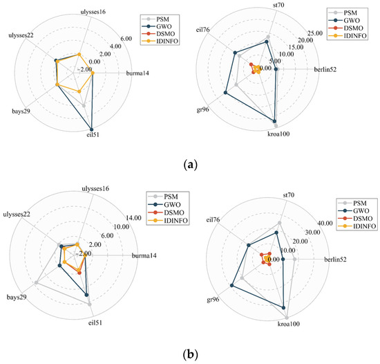
Figure 6.
Radar chart. (a) Deviation rate of the best solutions and (b) deviation rate of the average solutions.
The aforementioned comparison has primarily focused on small-scale data sets. To further investigate the performance of IDINFO, we conduct a comparative analysis with DSMO, DJAYA (Discrete JAYA), and AGA (Active Genetic Algorithm) algorithms on medium-sized instances. The results obtained from DSMO are consistent with those reported in Reference [43]. DJAYA is a novel discrete meta-heuristic algorithm that exhibits strong competitiveness and robustness in solving TSPs, surpassing even the latest algorithms [44]. AGA, on the other hand, is a cutting-edge genetic optimization algorithm that offers a superior solution to other methods in solving complex problems, with great accuracy and robustness [45]. It is noteworthy that the experimental results of DJAYA and AGA only present the average tour costs, which are obtained from 20 and 25 repeated tests, respectively. This is similar to our approach, which also takes an average of 20 repeated tests. As such, any potential error in this regard is negligible.
Table 7 presents a comparison of the average tour cost of the four algorithms across 22 TSP instances. The optimal values (i.e., minimum cost) of the four algorithms are highlighted, and the horizontal line representation algorithm is not tested in this dataset. Notably, the DSMO algorithm is tested on a lot of instances, reaching 493 points. While DSMO performs comparably to IDINFO on small-scale datasets, such as eil51 and berlin52, our method outperforms DSMO in all instances. As the data size increases, the gap between DSMO and the proposed method becomes even more pronounced, as observed in pr124 and pr439. The DJAYA algorithm is tested on 10 TSP use cases, with the maximum number of points being 225. Compared with DJAYA, IDINFO performs only slightly worse on berlin52 and ch150, with the gap being less than 0.6%. In the remaining eight instances, our method outperforms DJAYA. On the other hand, except for the eil76 dataset, the AGA algorithm exhibits a significant gap with our method in all other results, with the average tour cost being up to 8.3% higher than IDINFO. Therefore, based on the test results across different small- and medium-sized TSP instances, IDINFO is superior to the other three algorithms in terms of average value and exhibits excellent comprehensive performance.
4.2.2. Comparison with Artificial Intelligence-Based Methods
In recent years, artificial intelligence-based methods have emerged as a prominent technology with applications in solving the TSP. In this section, we present a comparison between the IDINFO algorithm and several typical intelligence-based methods, including CNO_PSO, Neural-3-OPT, LIH (learning improvement heuristics), AM (Attention model), and UTSP for solving the TSP. Specifically, the CNO_PSO algorithm is proposed to solve the TSP based on continuous Hopfield Neural Network (HNN) and PSO algorithm [46]. It performed well in small-scale TSP instances. Neural-3-OPT is an iterative improvement method that uses deep reinforcement learning to automatically learn effective 3-opt local search for solving the TSP [47]. It achieved the most advanced performance among existing neural network-based methods on real and randomly generated TSP instances. Wu et al. [48] propose a deep reinforcement learning framework for directly learning improvement heuristics (LIH) for the routing problem. Experimental results demonstrate that LIH learns more effective and generalizable strategies, thereby significantly surpassing certain advanced DL-based approaches in solving the TSP. AM [40] (Attention Model) is a network model based on the attention mechanism in Transformer, combined with the REINFORCE method for training, which significantly improves the performance of learning-based algorithms for combinatorial optimization problems such as the TSP. UTSP [49] is an unsupervised learning framework that uses Graph Neural Networks (GNN) to generate heatmaps and employs local search to generate the final prediction. It significantly enhances parameter efficiency, data efficiency, and training speed and can directly handle large-scale TSP instances.
Table 8 presents a comparison of the best solutions obtained by IDINFO, CNO_PSO, Neural-3-OPT, LIH, AM, and UTSP algorithms in 21 TSP cases. The algorithm results of CNO_PSO, Neural-3-OPT, LIH, AM, and UTSP are sourced from the literature. The horizontal line in Table 8 indicates that the algorithm is not tested under that instance, and no results are obtained.
Table 8.
Comparison of IDINFO with CNO_PSO, Neural-3-OPT, LIH, AM, and UTSP on TSP instances.
As shown in Table 8, CNO-PSO focuses on small-scale instances with city nodes not exceeding 48. In comparison, the IDINFO algorithm generates higher-quality optimal solutions, especially for the ulysses22 and att48 datasets. On these two datasets, the CNO-PSO computation yields the best route lengths, 22% and 34% higher than the IDINFO algorithm, indicating significant differences. On the other hand, the Neural-3-OPT algorithm is tested on nine larger-scale datasets, and IDINFO still demonstrates better solutions for most instances, slightly inferior only to Neural-3-OPT on the eil101 instance. For 51 to 280 city nodes, the route length of IDINFO is at least 7.14 shorter than that of Neural-3-OPT, with a maximum reduction of 1934.24. The LIH algorithm is extensively tested on datasets with up to 299 nodes and performs exceptionally well. However, it only outperforms the IDINFO algorithm on the rd100 instance while falling short on the remaining 20 instances. Additionally, AM and UTSP also perform weaker than IDINFO on medium and small-scale datasets. For datasets with city sizes under 200, IDINFO outperforms both AM and UTSP. However, we tested the performance of these algorithms on large-scale datasets, and the results show that IDINFO outperforms AM on pr439 but performs worse than UTSP on d493. This indicates that IDINFO may need further improvement for large-scale datasets.
Overall, the testing results of IDINFO are superior to other algorithms in most instances, showcasing its best overall performance.
4.3. The Application of IDINFO in Short-Distance Delivery Scenarios
To further validate the practicality and effectiveness of the IDINFO algorithm in realistic urban spatial scenarios, we applied both the DINFO and the IDINFO to the urban road network to solve the TSP in short-distance delivery scenarios.
We evaluate IDINFO in two experimental areas with different road network complexities to validate its path optimization capability in short-distance delivery scenarios and its adaptability in road environments affected by obstacles. Both experimental areas are based on road data from the OSM (OpenStreetMap) platform, with 20 randomly selected delivery points for couriers (indicated by yellow circles in the figures). The shortest paths are calculated using the Dijkstra algorithm [50], and a cost matrix is constructed as the data basis for algorithm testing. Experimental Area 1 covers 4.6487 km2, with 772 road nodes and 1088 road segments, as shown in Figure 7. Experimental Area 2 covers 9.4326 km2, with 1364 road nodes and 2236 road segments, as shown in Figure 8. To further assess the adaptability of IDINFO in road environments affected by obstacles, 10 obstacle points are specifically set in Experimental Area 2 to simulate road closures or temporary construction scenarios that may occur during actual delivery processes (indicated by red triangles in Figure 8).
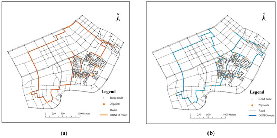
Figure 7.
Route planning results in Experimental Area 1, (a) the best route of IDINFO, and (b) the best route of DINFO.
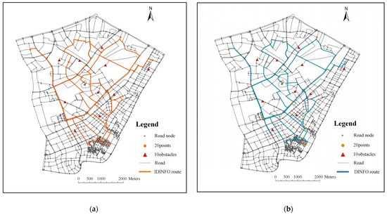
Figure 8.
Route planning results in Experimental Area 2 with obstacles, (a) the best route of IDINFO, and (b) the best route of DINFO.
Using the shortest route length as the goal, Figure 7 shows the routes planned by DINFO and IDINFO based on the urban road network. The route lengths planned by IDINFO and DINFO were 11,334.20 m and 12,307.66 m, respectively, with convergence times of 2.11 s and 13.13 s. The route planned by IDINFO was 973.46 m shorter than DINFO, with a time consumption of 11.02 s less than DINFO. Additionally, Figure 8 shows the routes planned by DINFO and IDINFO in larger and more complex scenarios considering obstacles. The route lengths planned by IDINFO and DINFO are 51,817.36 m and 53,731.43 m, respectively, with convergence times of 14.27 s and 41.9 s. The route planned by IDINFO is 1914.07 m shorter than DINFO, with a time consumption of 27.63 s less than DINFO.
This application of the IDINFO algorithm indicates that it can be successfully applied in real space to quickly and effectively find the optimal route for the TSP. The experimental results show that IDINFO can not only significantly optimize path planning in standard short-distance distribution tasks but also maintain high solution efficiency and path quality in road environments interfered by obstacles, further proving its practicability in urban logistics, intelligent scheduling and other geoinformatics practical applications.
5. Conclusions
In this paper, we present a novel algorithm, IDINFO, for solving TSPs. IDINFO introduces several improvements to the original INFO, including redefined operators, optimized updating rule stage, and multi-strategy local search. Additionally, IDINFO incorporates threshold-based 2-opt and 3-opt local search techniques. We evaluate IDINFO using abundant instances with different features. Results show that it significantly reduces time consumption, improves solution accuracy and optimization speed, and performs well on small and medium-sized instances. Compared to popular metaheuristic algorithms such as PSM, GWO, DSMO, DJAYA, AGA, and artificial intelligence-based methods such as CNO_PSO, Neural-3-OPT, LIH, AM, and UTSP, IDINFO demonstrates superior performance. However, it still needs to be improved for large-scale datasets. In addition, this paper gives the specific application of IDINFO. Future work will focus on two aspects: one is to optimize the IDINFO algorithm to enhance its ability to solve large-scale TSPs while maintaining the accuracy of the solution, and the other is to explore more use cases of IDINFO to solve specific geographical problems.
Author Contributions
Conceptualization, Yichun Su and Zhao Yan; methodology, Zhao Yan; software, Xue Yang; validation, Yichun Su, Zhao Yan, and Yunbo Ran; formal analysis, Yunbo Ran; investigation, Yichun Su; resources, Yunbo Ran; data curation, Zhao Yan; writing—original draft preparation, Zhao Yan and Yunbo Ran; writing—review and editing, Yichun Su and Xue Yang; visualization, Zhao Yan; supervision, Xue Yang, Yunfei Zhang; project administration, Xue Yang, Yunfei Zhang; funding acquisition, Xue Yang. All authors have read and agreed to the published version of the manuscript.
Funding
This work was funded by the National Natural Science Foundation of China (No.42271449).
Data Availability Statement
The data used in this study can be made available by contacting the corresponding author.
Acknowledgments
The authors would like to sincerely thank the anonymous reviewers for their constructive comments and valuable suggestions to improve the quality of this article.
Conflicts of Interest
The authors declare no conflicts of interest.
Abbreviations
The following abbreviations are used in this manuscript:
| IDINFO | Improved version of the discretized INFO |
| INFO | Weighted mean of vectors |
| TSP | Traveling salesman problem |
| PSM | Producer scrounger method |
| GWO | Grey wolf optimization |
| DSMO | Discrete spider monkey optimization |
| DJAYA | Discrete JAYA |
| AGA | Active genetic algorithm |
| PSO | Particle swarm optimization |
| CNO_PSO | Collective neurodynamic optimization PSO |
| LIH | Learning improvement heuristics |
| IP | Integer programming |
| NN | Nearest neighbor |
| DRL | Deep reinforcement learning |
| SI | Swarm intelligence |
| SSA | Sparrow search algorithm |
| SCA | Sine cosine algorithm |
| BnB | Branch and bound |
| DP | Dynamic programming |
| NCO | Neural combinatorial optimization |
| GPNs | Graph pointer networks |
| NETSP | Non-Euclidean TSP network |
| GCE-MAD Net | Graph convolutional encoder and multi-headed attention decoder network |
| GA | Genetic algorithm |
| MA | Memetic algorithm |
| DE | Differential evolution |
| SSO | Swallow swarm optimization |
| WOA | Whale optimization algorithm |
| SSA | Swallow search algorithm |
| ACO | Ant colony optimization |
| SA | Simulated annealing |
| HNN | Hopfield neural network |
References
- Hou, T.; Su, C.; Chang, H. An Integrated Multi-Objective Immune Algorithm for Optimizing the Wire Bonding Process of Integrated Circuits. J. Intell. Manuf. 2008, 19, 361–374. [Google Scholar] [CrossRef]
- Hua, X.; Hu, X.; Yuan, W. Research Optimization on Logistics Distribution Center Location Based on Adaptive Particle Swarm Algorithm. Optik 2016, 127, 8443–8450. [Google Scholar] [CrossRef]
- Liang, H.; Wang, S.; Li, H.; Zhou, L.; Zhang, X.; Wang, S. BiGNN: Bipartite graph neural network with attention mechanism for solving multiple traveling salesman problems in urban logistics. Int. J. Appl. Earth Obs. Geoinf. 2024, 129, 103863. [Google Scholar] [CrossRef]
- Farrag, T.A.; Askr, H.; Elhosseini, M.A.; Hassanien, A.E.; Farag, M.A. Intelligent Parcel Delivery Scheduling Using Truck-Drones to Cut down Time and Cost. Drones 2024, 8, 477. [Google Scholar] [CrossRef]
- Yan, J.; Zlatanova, S.; Lee, J.B.; Liu, Q. Indoor traveling salesman problem (itsp) path planning. ISPRS Int. J. Geo-Inf. 2021, 10, 616. [Google Scholar] [CrossRef]
- Rinaldi, M.; Primatesta, S.; Bugaj, M.; Rostáš, J.; Guglieri, G. Development of heuristic approaches for last-mile delivery TSP with a truck and multiple drones. Drones 2023, 7, 407. [Google Scholar] [CrossRef]
- Cheikhrouhou, O.; Khoufi, I. A Comprehensive Survey on the Multiple Traveling Salesman Problem: Applications, Approaches, and Taxonomy. Comput. Sci. Rev. 2021, 40, 100369. [Google Scholar] [CrossRef]
- Pop, P.C.; Cosma, O.; Sabo, C.; Sitar, C.P. A Comprehensive Survey on the Generalized Traveling Salesman Problem. Eur. J. Oper. Res. 2023, 314, 819–835. [Google Scholar] [CrossRef]
- Bello, I.; Pham, H.; Le, Q.V.; Norouzi, M.; Bengio, S. Neural Combinatorial Optimization with Reinforcement Learning. arXiv 2016, arXiv:1611.09940. [Google Scholar] [CrossRef]
- Ma, Q.; Ge, S.; He, D.; Thaker, D.; Drori, I. Combinatorial Optimization by Graph Pointer Networks and Hierarchical Reinforcement Learning. arXiv 2019, arXiv:1911.04936. [Google Scholar] [CrossRef]
- Vinyals, O.; Fortunato, M.; Jaitly, N. Pointer Networks. In Advances in Neural Information Processing Systems; Cortes, C., Lawrence, N., Lee, D., Sugiyama, M., Garnett, R., Eds.; Curran Associates, Inc.: New York, NY, USA, 2015; Volume 28. [Google Scholar] [CrossRef]
- Clerc, M. Discrete Particle Swarm Optimization, illustrated by the Traveling Salesman Problem. In New Optimization Techniques in Engineering; Onwubolu, G.C., Babu, B.V., Eds.; Springer: Berlin/Heidelberg, Germany, 2004; pp. 219–239. [Google Scholar] [CrossRef]
- Li, W.; Zhang, M.; Zhang, J.; Qin, T.; Wei, W.; Yang, J. A Multimixed Strategy Improved Sparrow Search Algorithm and Its Application in TSP. Math. Probl. Eng. 2022, 2022, 8171164. [Google Scholar] [CrossRef]
- Ahmadianfar, I.; Heidari, A.A.; Noshadian, S.; Chen, H.; Gandomi, A.H. INFO: An Efficient Optimization Algorithm Based on Weighted Mean of Vectors. Expert Syst. Appl. 2022, 195, 116516. [Google Scholar] [CrossRef]
- Blum, C.; Roli, A. Metaheuristics in Combinatorial Optimization: Overview and Conceptual Comparison. ACM Comput. Surv. 2003, 35, 268–308. [Google Scholar] [CrossRef]
- Applegate, D.; Cook, W.; Rohe, A. Chained Lin-Kernighan for Large Traveling Salesman Problems. INFORMS J. Comput. 2003, 15, 82–92. [Google Scholar] [CrossRef]
- Li, Y.; Ma, K.; Zhang, J. An Efficient Multicore Based Parallel Computing Approach for TSP Problems. In Proceedings of the 2013 Ninth International Conference on Semantics, Knowledge and Grids, Beijing, China, 3–4 October 2013; pp. 98–104. [Google Scholar] [CrossRef]
- Christofides, N. Worst-Case Analysis of a New Heuristic for the Travelling Salesman Problem. Oper. Res. Forum 2022, 3, 20. [Google Scholar] [CrossRef]
- Johnson, D.S. Local Optimization and the Traveling Salesman Problem. In Automata, Languages and Programming; Paterson, M.S., Ed.; Springer: Berlin/Heidelberg, Germany, 1990; pp. 446–461. [Google Scholar]
- Sultana, N.; Chan, J.; Sarwar, T.; Qin, A.K. Learning to Optimise General TSP Instances. Int. J. Mach. Learn. Cybern. 2022, 13, 2213–2228. [Google Scholar] [CrossRef]
- Luo, J.; Li, C.; Fan, Q.; Liu, Y. A Graph Convolutional Encoder and Multi-Head Attention Decoder Network for TSP via Reinforcement Learning. Eng. Appl. Artif. Intell. 2022, 112, 104848. [Google Scholar] [CrossRef]
- Dokeroglu, T.; Sevinc, E.; Kucukyilmaz, T.; Cosar, A. A Survey on New Generation Metaheuristic Algorithms. Comput. Ind. Eng. 2019, 137, 106040. [Google Scholar] [CrossRef]
- Wang, Y.; Gao, S.; Yu, Y.; Cai, Z.; Wang, Z. A Gravitational Search Algorithm with Hierarchy and Distributed Framework. Knowl. Based Syst. 2021, 218, 106877. [Google Scholar] [CrossRef]
- Derviş, K.; Selçuk, Ö. A Simple and Global Optimization Algorithm for Engineering Problems: Differential Evolution Algorithm. Turk. J. Electr. Eng. Comput. Sci. 2004, 12, 53–60. [Google Scholar]
- Qu, L.; Sun, R. A Synergetic Approach to Genetic Algorithms for Solving the Traveling Salesman Problem. Inf. Sci. 1999, 117, 267–283. [Google Scholar] [CrossRef]
- Seo, W.; Park, M.; Kim, D.-W.; Lee, J. Effective Memetic Algorithm for Multilabel Feature Selection Using Hybridization-Based Communication. Expert Syst. Appl. 2022, 201, 117064. [Google Scholar] [CrossRef]
- Bouzidi, S.; Riffi, M.E. Discrete Swallow Swarm Optimization Algorithm for Travelling Salesman Problem. In Proceedings of the 2017 International Conference on Smart Digital Environment, Rabat, Morocco, 21–23 July 2017; pp. 80–84. [Google Scholar] [CrossRef]
- Ahmed, O.M.; Kahramanli, H. Meta-Heuristic Solution Approaches for Traveling Salesperson Problem. Int. J. Appl. Math. Electron. Comput. 2018, 6, 21–26. [Google Scholar]
- Deng, W.; Zhang, L.; Zhou, X.; Zhou, Y.; Sun, Y.; Zhu, W.; Chen, H.; Deng, W.; Chen, H.; Zhao, H. Multi-Strategy Particle Swarm and Ant Colony Hybrid Optimization for Airport Taxiway Planning Problem. Inf. Sci. 2022, 612, 576–593. [Google Scholar] [CrossRef]
- Raghavendran Dr, C.V.; Satish, G.; Penumathsa, S.V. Intelligent Routing Techniques for Mobile Ad hoc Networks using Swarm Intelligence. Int. J. Intell. Syst. Appl. 2012, 5, 81–89. [Google Scholar] [CrossRef]
- Yang, J.; Shi, X.; Marchese, M.; Liang, Y. An Ant Colony Optimization Method for Generalized TSP Problem. Prog. Nat. Sci. 2008, 18, 1417–1422. [Google Scholar] [CrossRef]
- Zhang, H.; Zhang, K.; Zhou, Y.; Ma, L.; Zhang, Z. An Immune Algorithm for Solving the Optimization Problem of Locating the Battery Swapping stations. Knowl. -Based Syst. 2022, 248, 108883. [Google Scholar] [CrossRef]
- Mirjalili, S. SCA: A Sine Cosine Algorithm for Solving Optimization Problems. Knowl. -Based Syst. 2016, 96, 120–133. [Google Scholar] [CrossRef]
- Lee, J.; Perkins, D. A Simulated Annealing Algorithm with a Dual Perturbation Method for Clustering. Pattern Recognit. 2021, 112, 107713. [Google Scholar] [CrossRef]
- Tzanetos, A.; Dounias, G. Nature Inspired Optimization Algorithms or Simply Variations of Metaheuristics? Artif. Intell. Rev. 2021, 54, 1841–1862. [Google Scholar] [CrossRef]
- Croes, G.A. A Method for Solving Traveling-Salesman Problems. Oper. Res. 1958, 6, 791–812. [Google Scholar] [CrossRef]
- Gülcü, Ş.; Mahi, M.; Baykan, Ö.K.; Kodaz, H. A Parallel Cooperative Hybrid Method Based on Ant Colony Optimization and 3-Opt Algorithm for Solving Traveling Salesman Problem. Soft Comput. 2018, 22, 1669–1685. [Google Scholar] [CrossRef]
- Helsgaun, K. An Effective Implementation of the Lin–Kernighan Traveling Salesman Heuristic. Eur. J. Oper. Res. 2000, 126, 106–130. [Google Scholar] [CrossRef]
- Reinelt, G. TSPLIB—A Traveling Salesman Problem Library. INFORMS J. Comput. 1991, 3, 376–384. [Google Scholar] [CrossRef]
- Kool, W.; Van Hoof, H.; Welling, M. Attention, learn to solve routing problems! arXiv 2018, arXiv:1803.08475. [Google Scholar]
- Akhand MA, H.; Hossain, F. Producer-Scrounger Method to Solve Traveling Salesman Problem. I.J. Intell. Syst. Appl. 2015, 7, 29–36. [Google Scholar] [CrossRef]
- Sopto, D.S.; Ayon, S.I.; Akhand MA, H.; Siddique, N. Modified Grey Wolf Optimization to Solve Traveling Salesman Problem. In Proceedings of the 2018 International Conference on Innovation in Engineering and Technology (ICIET), Dhaka, Bangladesh, 27–28 December 2018; pp. 1–4. [Google Scholar] [CrossRef]
- Akhand, M.A.H.; Ayon, S.I.; Shahriyar, S.A.; Siddique, N.; Adeli, H. Discrete Spider Monkey Optimization for Travelling Salesman Problem. Appl. Soft Comput. 2020, 86, 105887. [Google Scholar] [CrossRef]
- Gunduz, M.; Aslan, M. DJAYA: A Discrete Jaya Algorithm for Solving Traveling Salesman Problem. Appl. Soft Comput. 2021, 105, 107275. [Google Scholar] [CrossRef]
- Jain, R.; Singh, K.P.; Meena, A.; Rana, K.B.; Meena, M.L.; Dangayach, G.S.; Gao, X.-Z. Application of Proposed Hybrid Active Genetic Algorithm for Optimization of Traveling Salesman Problem. Soft Comput. 2023, 27, 4975–4985. [Google Scholar] [CrossRef]
- Zhong, J.; Feng, Y.; Tang, S.; Xiong, J.; Dai, X.; Zhang, N. A Collaborative Neurodynamic Optimization Algorithm to Traveling Salesman Problem. Complex Intell. Syst. 2023, 9, 1809–1821. [Google Scholar] [CrossRef]
- Sui, J.; Ding, S.; Liu, R.; Xu, L.; Bu, D. Learning 3-opt Heuristics for Traveling Salesman Problem via Deep Reinforcement Learning. In Proceedings of the 13th Asian Conference on Machine Learning, Virtual, 17–19 November 2021; Balasubramanian, V.N., Tsang, I., Eds.; Volume 157, pp. 1301–1316, PMLR. [Google Scholar] [CrossRef]
- Wu, Y.; Song, W.; Cao, Z.; Zhang, J.; Lim, A. Learning Improvement Heuristics for Solving Routing Problems. IEEE Trans. Neural Netw. Learn. Syst. 2022, 33, 5057–5069. [Google Scholar] [CrossRef] [PubMed]
- Min, Y.; Bai, Y.; Gomes, C.P. Unsupervised learning for solving the travelling salesman problem. Adv. Neural Inf. Process. Syst. 2024, 36, 47264–47278. [Google Scholar]
- Dijkstra, E.W. A Note on Two Problems in Connexion with Graphs. Numer. Math. 1959, 1, 269–271. [Google Scholar] [CrossRef]


Disclaimer/Publisher’s Note: The statements, opinions and data contained in all publications are solely those of the individual author(s) and contributor(s) and not of MDPI and/or the editor(s). MDPI and/or the editor(s) disclaim responsibility for any injury to people or property resulting from any ideas, methods, instructions or products referred to in the content. |
© 2025 by the authors. Published by MDPI on behalf of the International Society for Photogrammetry and Remote Sensing. Licensee MDPI, Basel, Switzerland. This article is an open access article distributed under the terms and conditions of the Creative Commons Attribution (CC BY) license (https://creativecommons.org/licenses/by/4.0/).