Geographic Distribution of Lung and Bronchus Cancer Mortality and Elevation in the United States: Exploratory Spatial Data Analysis and Spatial Statistics

Abstract

Lung and bronchus cancer, collectively called lung cancer, remains one of the most lethal malignancies worldwide, with its incidence and mortality rates continuing to pose significant public health challenges. Numerous studies have explored various risk factors for lung cancer, including smoking, environmental pollutants, genetic predispositions, and occupational hazards. However, emerging research suggests that elevation above sea level may also influence lung and bronchus cancer prevalence and outcomes. We analyzed elevation data for 2662 contiguous U.S. counties to determine if there is a significant relationship between lung cancer and elevation. Moreover, we employed hierarchical multiple regression and a complex sample general linear model (CSGLM) to enhance the understanding of the factors influencing lung and bronchus cancer, with a particular focus on elevation. Using Local Moran’s I cluster analysis, we identified statistically significant hot spots and cold spots for the mortality rate related to lung cancer. In the hierarchical regression model, a significant correlation between lung cancer and elevation remained evident. This suggests that the risk of mortality from lung and bronchus cancer increases with decreasing elevation (R² = 0.601). Furthermore, within the CSGLM framework, an R² value of 0.763 highlighted a strong link between lung cancer mortality and elevation. This relationship remained significant even after accounting for complex sample designs and applying weight adjustments. This geographic correlation has not been documented in previous studies. Further research is necessary to elucidate the precise mechanisms through which elevation influences lung cancer biology.

1. Introduction

Lung-bronchus cancer, collectively known as lung cancer, remains one of the most prevalent and deadly forms of cancer worldwide. According to the World Health Organization (WHO), lung cancer is the leading cause of cancer mortality, accounting for approximately 1.8 million deaths annually, which represents about 18% of all cancer deaths [1]. According to projections by the American Cancer Society, in 2023, the United States sees approximately 238,340 new cases of lung and bronchus cancer, with an estimated 127,070 deaths resulting from the disease. Data from 2017–2019 indicates that about 6.1 percent of men and women will receive a prognosis of lung and bronchus cancer in their lifetime [2,3]. The high mortality rate is primarily due to the disease’s typically late diagnosis and its aggressive nature.

The largest risk factor for lung cancer is tobacco smoking, responsible for about 85–90% of lung cancer cases. Other significant risk factors include exposure to radon gas, asbestos, and other carcinogens, as well as genetic predispositions and environmental pollutants [4]. Although lung cancer is closely linked to cigarette smoking, only approximately 15% of smokers develop the disease, and 10–15% of lung cancer cases occur in nonsmokers [5,6]. Such discrepancies in findings may be caused by various confounding factors and methodological challenges. For instance, differences in population genetics, lifestyle factors, smoking prevalence, healthcare access, and environmental exposures can all influence lung cancer risk and outcomes [7]. Moreover, data quality and differences in study design can also impact the results and their interpretation.

Elevation, an often-overlooked environmental factor, has gained increasing attention for its potential role in shaping cancer outcomes. Previous studies have suggested that the interplay between elevation and environmental factors, such as air quality, oxygen availability, and ultraviolet (UV) radiation exposure, may contribute to variations in lung-bronchus cancer death rates [8,9]. However, the specific mechanisms underlying these associations remain inadequately explored, underscoring the need for further research.

In addition, elevation is associated with unique environmental characteristics, including reduced oxygen levels (hypoxia), lower barometric pressure, and decreased air pollution. Hypoxia, which is a hallmark of high-elevation environments, may have biological effects that influence cancer development and progression. Research suggests that hypoxic conditions at higher elevations can alter tumor metabolism, angiogenesis, and cellular signaling pathways, potentially inhibiting the growth and spread of cancers, including lung cancer [9,10,11]. Additionally, higher elevations are often characterized by cleaner air with lower levels of particulate matter (PM2.5) and other air pollutants, which are established risk factors for lung cancer [12]. These environmental factors collectively create conditions that may protect against the incidence and severity of lung cancer in populations residing at higher elevations.

Nevertheless, the differences in lung cancer mortality rates across regions in the United States, along with the link between lung cancer and elevation, are still not fully understood. The relationship between geographic location and negative health outcomes is complex and multifaceted. Recent studies have begun to shed light on this prominent issue, investigating the disparities in various health outcomes, including lung cancer, across different geographic areas [13,14,15].

Moreover, in survey research, particularly when dealing with complex survey data, the application of statistical techniques such as stratification, clustering, and weighting is crucial for obtaining accurate, representative, and reliable results. These methods address the intricacies of survey designs and help mitigate biases, ensuring that the findings reflect the true characteristics of the population under study. Nevertheless, many researchers often handle these surveys as though they were unweighted simple random samples, which can lead to biased variance estimates and a higher risk of Type I errors [16,17,18]. In complex survey data, the combined use of stratification, clustering, and weighting addresses various challenges, including improved precision and accuracy. These methods are indispensable techniques in the analysis of complex survey data. They ensure that survey estimates are precise, unbiased, and representative of the population, thereby enhancing the reliability and validity of the survey findings [16,17,18]. Software packages such as SPSS 22 and Stata 17 now feature modules that can adjust variance estimates for general linear models, logistic regressions, and ordinal regressions when dealing with complex sample designs [19,20].

Applying spatial regression in health studies is crucial for understanding and addressing geographic variations in health outcomes. Traditional regression models often fail to account for spatial dependencies, where health outcomes in one area may be influenced by those in neighboring regions. Spatial regression techniques correct for this spatial autocorrelation, leading to more accurate and unbiased estimates [21]. This is essential for identifying regional health disparities and environmental impacts on health, which can inform targeted public health interventions and resource allocation [22]. By incorporating spatial regression, health studies can better capture the complex spatial patterns inherent in health data, leading to an improved understanding and more effective interventions [23].

2. Materials and Methods

2.1. Lung-Bronchus Cancer Mortality Data

This study examines the hypothesis that elevation significantly contributes to lung and bronchus cancer mortality by considering the impact of related risk factors. To test this hypothesis, data on age-adjusted lung and bronchus cancer mortality rates from 2016–2020 were gathered from State Cancer Profiles. Mortality data were sourced from the National Vital Statistics System public data file, and death rates were calculated by the National Cancer Institute using the SEER Stat. These death rates (deaths per 100,000 population per year) are adjusted to the 2010 US Standard population. Figure 1 presents lung and bronchus cancer mortality rates across 2662 contiguous counties from 2016 to 2020.

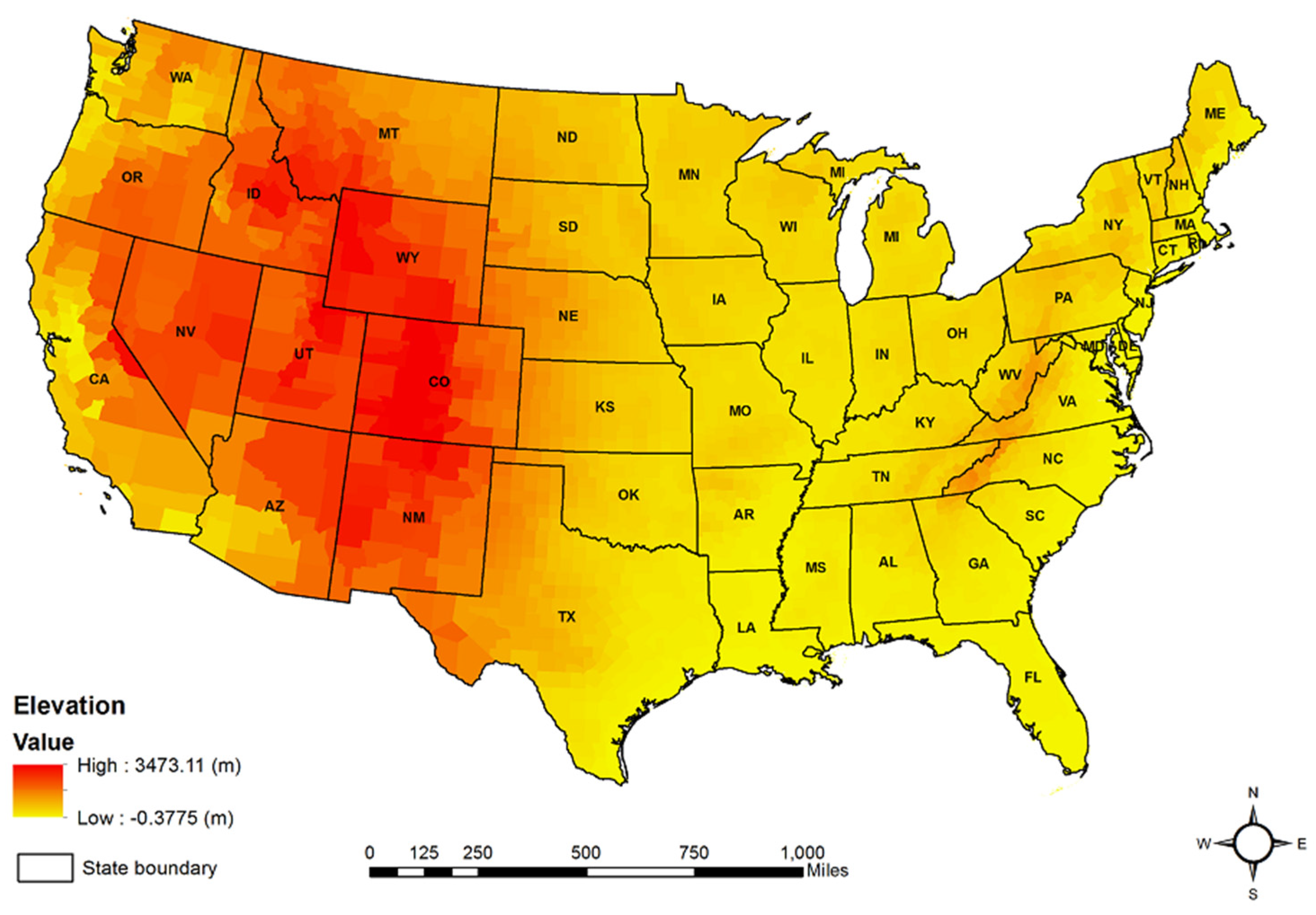
2.2. Mean County Elevation Data

County elevation data for 3141 administrative areas within the U.S. was created by the U.S. Geological Survey [24]. The mean elevation for each county was accurately calculated using the 100 m spatial resolution of the USGS dataset. Zonal statistics within the ArcGIS 10.5 were utilized to compute the mean elevation for each county, minimizing variations in topography. This method is more reliable, even for large counties, although challenges are more pronounced when considering entire states [25] or using elevation values from the county centers [26]. The analysis included data from 3064 contiguous counties. County boundaries from the U.S. Census Bureau were used to obtain the mean county elevations in meters and the area in square miles for each county, as illustrated in Figure 2.

2.3. Potential Confounders

To improve the reliability of our analyses, we accounted for several confounding factors as detailed by other lung-bronchus cancer studies [27,28,29]. These include: (1) health behavior factors like the percentage of adult smokers, insufficient sleep, adult obesity, the food environment index, physical inactivity, and alcohol impairment; (2) clinical care factors, such as the proportion of uninsured individuals, the ratio of primary care physicians to the population, and rates of preventable hospitalizations; (3) social and economic factors, including the percentage of the population with a college education, unemployment rates, household income at the 80th percentile, and the number of membership associations per 10,000 people; (4) physical environmental factors, such as the average daily PM2.5 concentration; and (5) demographic factors, including the percentage of individuals aged 65 and older, the proportion of African American residents, the percentage of female residents, and the proportion of the population living in rural areas. Due to the limited availability of variables related to mental health conditions in the SMART BRFSS, we had to source data on potential confounding factors from various other datasets [30].

For health behaviors, such as the percentage of adult smokers and obesity rates, data were obtained from both the BRFSS and the CDC Diabetes Interactive Atlas. Clinical care information, including the ratio of uninsured adults and the ratio of primary care physicians, was retrieved from the Small Area Health Insurance Estimates (SAHIE) and the American Medical Association (AMA). Data on preventable hospital stays was sourced from the Dartmouth Atlas of Health Care. Additionally, information on the percentage of individuals holding a college degree was gathered from the American Community Survey (ACS), while data on social associations came from the County Business Patterns. Lastly, demographic factors such as the percentage of adults aged 65 and older, the percentage of African Americans, the percentage of females, and the percentage of rural residents were all obtained from Census Population Estimates [30]. Most of these covariates from different database sources used ACS 5-year estimates from 2010–2014 and Census Population Estimates in 2014 to be consistent with the time frame of the SMART BRFSS and lung-bronchus cancer mortality data.

2.4. Model Analysis

This study was conducted in three steps to examine the variations in the relationship between lung-bronchus cancer mortality rates and elevation over different geographic areas. In the initial stage, we evaluated the skewness of dependent variables before data analysis to ascertain if any variables needed transformation, concluding that no transformation was required (Skewness = 0.585). In the second stage, we integrated elevation with potential confounding factors on lung-bronchus cancer into a stepwise regression model. In addition, multicollinearity in our predictors was evaluated using the variance inflation factor (VIF) [31]. Our primary objective was to investigate the relationship between lung-bronchus cancer mortality rates and elevation, so we employed a hierarchical multiple regression model. Firstly, the model included only the elevation. In the next step, we added potential confounding factors in a second regression model to ensure that their inclusion did not alter the significance of elevation in affecting the lung-bronchus cancer mortality rate. In the final stage, it is critical to analyze all BRFSS data, including SMART data, using statistical methods that account for the complex sampling design and weighting adjustments. This step is vital to avoid incorrect variance estimates and to reduce the likelihood of Type I errors (false positives) [19,20]. To accomplish this, we utilized the Complex Samples General Linear Model (CSGLM) in SPSS 22. This approach adjusts variance estimates for GLM within complex sample designs [14].

2.5. Local Mortan’s I Analysis

Local Moran’s I is a powerful tool used in spatial statistics to identify clusters or outliers of spatial data. Unlike the global Moran’s I, which provides a single measure of spatial autocorrelation for an entire dataset, Local Moran’s I focuses on individual locations, revealing the local patterns of spatial association. This local indicator of spatial association (LISA) is instrumental in pinpointing specific areas of high or low values that deviate significantly from the overall spatial pattern [32]. The Local Moran’s I helps in identifying local clusters (high-high or low-low) and spatial outliers (high-low or low-high). Spatial analysis software, such as ArcGIS, GeoDa, and R, provides tools for computing Local Moran’s I and visualizing the results through cluster maps. These visualizations are crucial for interpreting the spatial patterns and making informed decisions based on the analysis [33].

3. Results

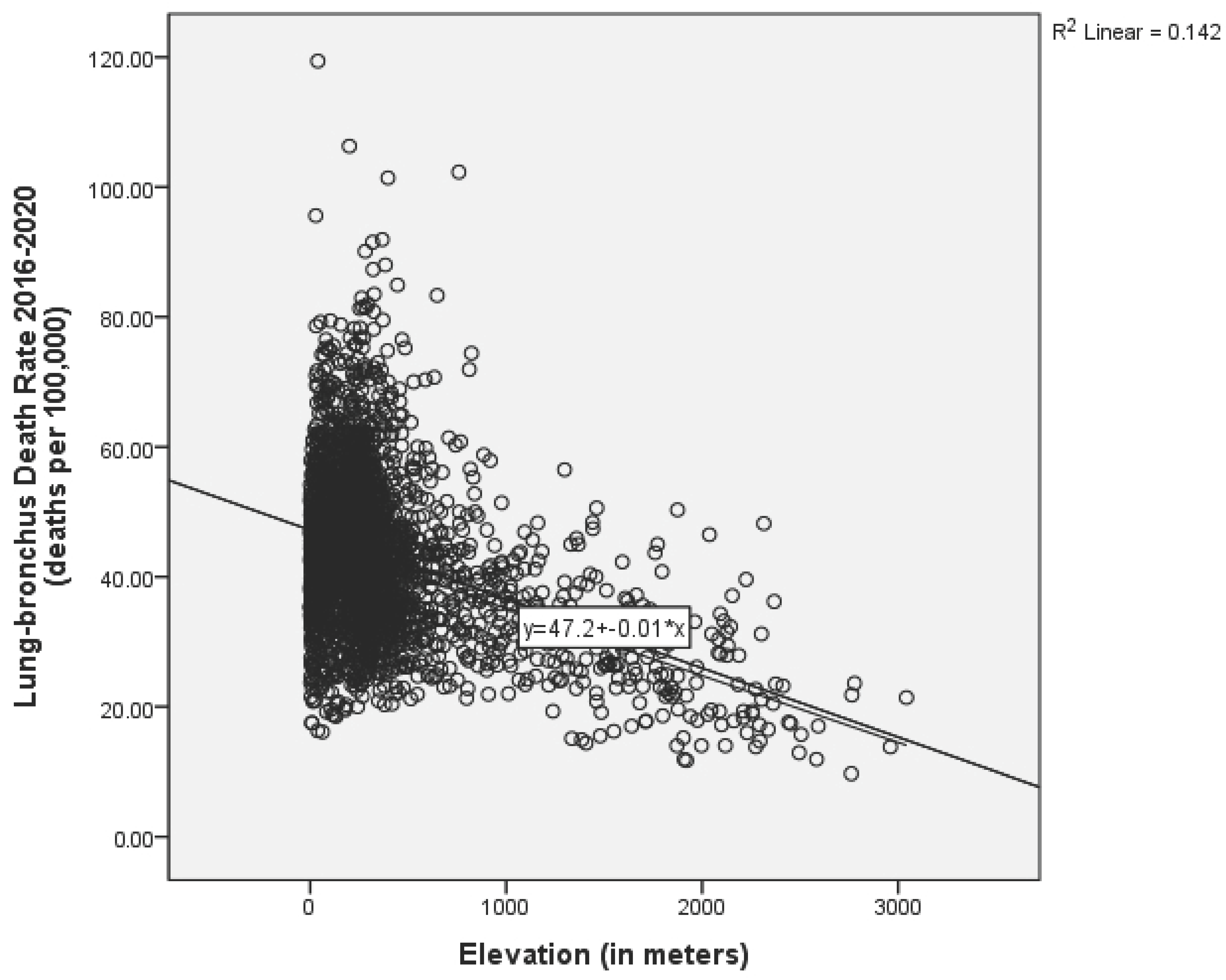
3.1. Descriptive and Bivariate Statistics

Table 1. Descriptive and bivariate statistics for dependent and independent variables.

	N	Mean	SD	Bivariate
Dependent variable:
Lung-Bronchus cancer death rate	2662	43.095	12.320	1.000 **
Independent variables:
Health behaviors:
% adult smoking	2662	18.601	3.645	0.647 **
% insufficient sleep	2662	33.460	3.962	0.439 **
% adult obesity	2662	31.181	4.469	0.566 **
Food environment index	2662	7.052	1.098	−0.290 **
% physically inactive	2662	27.403	5.490	0.637 **
% alcohol impaired		30.827	12.965	−0.018
Clinical care:
% uninsured	2662	16.955	5.103	0.110 **
Primary care physician ratio	2662	56.298	32.420	−0.300 **
Preventable hospital stays	2662	63.482	24.646	0.573 **
Social economic environment:
% of college education	2662	56.034	11.167	−0.469 **
% unemployment	2662	6.460	2.121	0.355 **
80th percentile income	2662	88,987.691	20,137.157	−0.504 **
Association rate	2662	13.094	5.291	0.019
Physical environment:
Average daily PM2.5	2662	11.700	1.524	0.297 **
Elevation	2662	373.160	439.119	−0.382 **
Demographics:
% 65 and over	2662	17.248	4.109	0.108 **
% African American	2662	9.874	14.725	0.136 **
% Female	2662	50.133	1.980	0.006
% Rural	2662	53.824	29.558	0.368 **

Abbreviation: SD, Standard Deviation; ** Significant at p > 0.05.

provides the mean, standard deviations (SD), and bivariate statistics of both dependent and independent variables. For dependent variables, average age-adjusted lung and bronchus cancer mortality rate (deaths per 100,000) in 2662 contiguous counties was 43.095 with a SD of 12.320. The mean county elevation was 373.160 m with a SD of 439.119 m. For health behavior factors, on average, 18.60% of a county’s adult participants were smokers with a SD of 3.64%. Also, on average, 33.46% and 31.18% of adult participants in the counties had insufficient sleep and obesity, with a SD of 3.96% and 4.46%, respectively. Moreover, the percentage of physically inactive and the percentage of alcohol impaired were, on average, 27.40% and 30.82%, with a SD of 5.49% and 12.96%, respectively. For clinical factors, on average, the percentage of uninsured and the number of primary care physicians per 100,000 patients were 16.95% and 56.29 physicians with a SD of 5.10% and 32.42 physicians, respectively. Also, preventable hospital stays, on average, were 63.48 hospital stays per 1000 patients with a SD of 24.64. For socioeconomic factors, the percentage of adults with a college education and the percentage of unemployed adults, on average, were 56.03% and 6.46% with a SD of 11.16% and 2.12%, respectively. Moreover, the mean county association rate was 13.83 membership associations per 100,000 population with a SD of 6.78. For demographic factors, the proportion of a county’s population aged 65 and above was, on average, 17.24% with a SD of 4.10%. The African American population, on average, accounted for 9.87% of a county’s population, with a SD of 14.72%. The variations in these independent variables indicate that lung-bronchus cancer mortality occurred in counties with heterogeneous behavioral, socio-demographic, and environmental characteristics. Furthermore, Figure 3 presents a scatter plot of lung-bronchus cancer death rates with elevation to show the possible association between two variables.

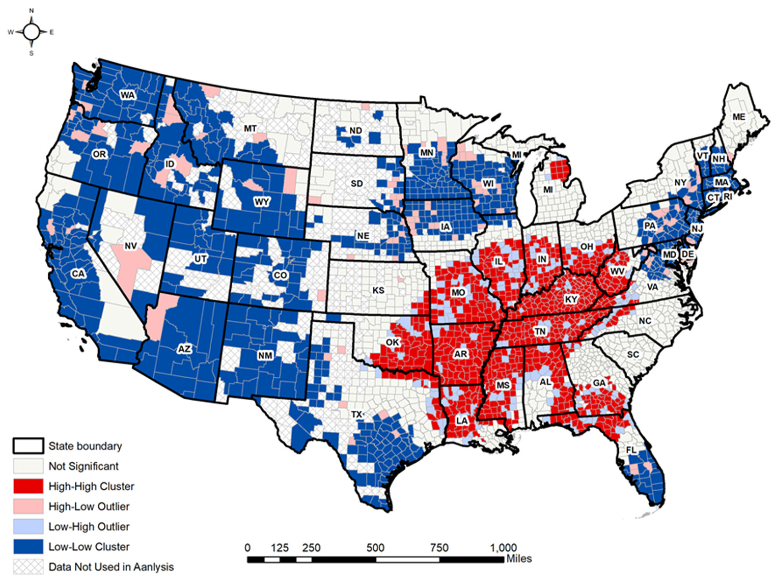
3.2. Local Moran’s I Analyses

Figure 4 illustrates the spatial distribution of local Moran’s I for lung-bronchus cancer mortality rates across the 48 contiguous states in the U.S. The high-high clusters, which represent areas with higher lung-bronchus cancer mortality, are mainly concentrated in the southeastern and central regions, including states like Alabama, Arkansas, Georgia, Kentucky, Louisiana, Mississippi, Missouri, Oklahoma, and Tennessee. These areas also report relatively lower levels of elevation. In contrast, the low-low clusters, or areas with lower lung-bronchus cancer mortality rates, are largely located in the Western and Midwestern parts of the country, especially in states such as Arizona, Colorado, Idaho, New Mexico, Utah, and Wyoming, which are placed at a relatively higher elevation. Additionally, the global Moran’s I test shows a value of 0.469 with a z-score of 109.355 and a p-value of less than 0.001, confirming that there is a statistically significant spatial clustering of lung-bronchus cancer death rates at the county level across the United States.

3.3. Hierarchical Regression Analyses

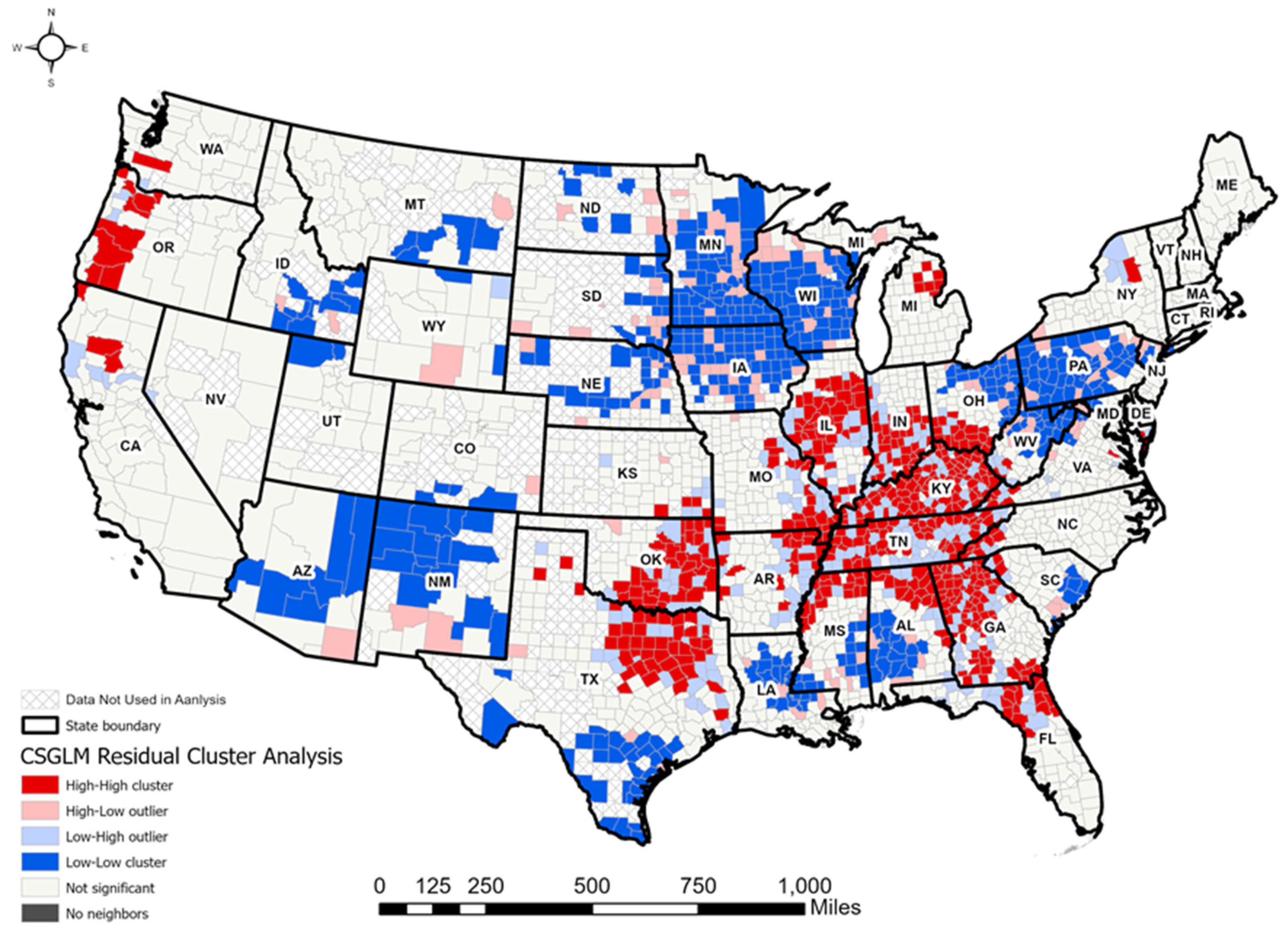
Model 1 demonstrated that the regression model only with the elevation factor was statistically significant, as indicated by an F-value of (1.2660) = 453.826 and a p-value of less than 0.001. As shown in

Table 2. Hierarchical regression models.

	Coefficient	S.E	t-Value	p-Value	95% C.I		VIF
Model 1—AIC: 13,077.853					Lower Bound	Upper Bound
Constant	47.093	0.290	162.550	0.000	46.525	47.661
Elevation	−0.011	0.001	−21.303	0.000 **	−0.012	−0.010	1.000
Model 2—AIC: 10,962.824
Constant	21.553	5.634	3.822	0.000	10.485	32.580
Health behaviors:
% adult smoking	0.793	0.077	10.284	0.000 **	0.642	0.944	3.444
% insufficient sleep	0.190	0.074	2.571	0.010 **	0.045	0.335	3.742
% adult obesity	0.087	0.060	1.457	0.145	−0.030	0.205	3.131
Food environment index	−1.209	0.245	−4.937	0.000 **	−1.689	−0.729	3.152
% physically inactive	0.389	0.052	7.554	0.000 **	0.288	0.490	3.486
% alcohol impaired	−0.014	0.012	−0.015	0.239	−0.037	0.009	1.036
Clinical care:
% uninsured	−0.310	0.045	−6.879	0.000 **	−0.399	−0.222	2.312
Primary care physician ratio	0.000	0.006	0.038	0.970	−0.011	0.012	1.625
Preventable hospital stays	0.077	0.008	9.182	0.000 **	0.061	0.094	1.879
Social economic environment:
% of college education	−0.046	0.026	1.791	0.073	−0.096	0.004	3.539
% unemployment	0.229	0.105	0.039	0.030 **	0.022	0.425	2.174
80th percentile income	−6.504 × 10−5	0.000	−4.467	0.000 **	0.000	0.000	3.747
Association rate	−0.096	0.058	−2.542	0.011 **	−0.170	−0.022	1.744
Physical environment:
Average daily PM2.5	0.503	0.127	3.945	0.000 **	0.253	0.752	1.644
Elevation	−0.006	0.000	−14.398	0.000 **	−0.007	−0.005	1.622
Demographics:
% 65 and over	0.119	0.053	2.232	0.026 **	0.014	0.224	2.096
% African American	−0.168	0.017	10.004	0.000 **	−0.201	−0.135	2.669
% Female	−0.013	0.088	−0.145	0.885	−0.185	0.159	1.312
% Rural	0.023	0.008	2.986	0.003 **	0.008	0.037	2.172

Abbreviation: SE, Standard Error; ** Significant at p > 0.05.

, the Akaike Information Criterion (AIC) value for the model was 13,077.853, which provides an estimate of model fit while penalizing complexity. A lower AIC value generally indicates a better-fitting model when comparing multiple models. Also, there was a significant relationship between elevation and lung-bronchus cancer mortality rate (β = −0.011; p = 0.000).

In Model 2, the subsequent hierarchical regression analysis included 19 variables and revealed that the overall model was statistically significant, with an F-value of (19.2642) = 209.227 and a p-value of less than 0.001. Results are further checked for multicollinearity among explanatory variables based on the variance inflation factor (VIF < 5), and all nineteen variables are included in the OLS model. Model 2, which incorporated all 19 independent variables, resulted in a significantly lower AIC value of 10,962.824. Since AIC penalizes model complexity while assessing fit, the lower AIC value in Model 2 suggests that incorporating additional predictors improves model performance compared to using elevation alone. Also, the regression analysis indicated that several variables were significantly associated with lung-bronchus cancer mortality rates, including elevation, percent of adult smokers, percent of insufficient sleep, food environment index, physical inactivity rate, percent of uninsured individuals, preventable hospital stays, percent of unemployment, 80th percentile income, association rate, average daily density of PM2.5, percent aged 65 and older, percent of African American individuals, and percent of rural residents, as illustrated in Table 2.

The results indicate that as the percentage of people residing at high elevation increases, the rate of mortality from lung-bronchus cancer decreases. Even after controlling for other potential confounding factors that might influence this relationship, elevation remained a significant predictor of lung-bronchus cancer mortality rates.

Moreover, the model residuals were spatially autocorrelated (Moran’s I = 0.113; z = 26.261; p < 0.001), meaning that the county-level lung-bronchus cancer death rates were spatially dependent across the 48 states. In addition, the residuals from the OLS model indicated that the lung-bronchus cancer death rates were underestimated primarily in the counties of southern states, including Kentucky, Georgia, Texas, and Oklahoma; and counties of western states, including Wyoming, Colorado, and Oregon (Figure 5).

3.4. CSGLM Analyses

The Complex Samples General Linear Model (CSGLM) technique is used to build on previous quantitative research exploring the link between lung-bronchus cancer mortality rates and elevation. This method considers complex sampling designs and adjusts for weights to provide accurate estimates of the key factors influencing lung-bronchus cancer mortality rates [10,24]. Model 3 in

Table 3. CSGLM regression models.

	Coefficient	S.E	t-Value	p-Value	95% C.I
Model 3—AIC: 11,225.379					Lower Bound	Upper Bound
Constant	35.512	9.082	3.577	0.000	16.045	54.980
Health behaviors:
% adult smoking	0.952	0.098	9.731	0.000 **	0.760	1.144
% insufficient sleep	−0.142	0.082	−1.739	0.082	−0.302	0.018
% adult obesity	0.297	0.118	2.507	0.012 **	0.065	0.529
Food environment index	−1.287	0.405	−3.175	0.002 **	−2.082	−0.492
% physically inactive	0.216	0.080	2.714	0.007 **	0.060	0.372
% alcohol impaired	0.060	0.019	3.209	0.001 **	0.024	0.097
Clinical care:
% uninsured	−0.340	0.088	−3.841	0.001 **	−0.513	−0.166
Primary care physician ratio	−1.099 × 10−5	0.007	−0.002	0.999	−0.013	0.013
Preventable hospital stays	0.092	0.014	6.769	0.000 **	0.065	0.118
Social economic environment:
% of college education	−0.015	0.038	−0.386	0.699	−0.089	0.060
% unemployment	0.058	0.165	0.350	0.726	−0.266	0.381
80th percentile income	−2.010 × 10−5	1.793 × 10−5	−1.121	0.262	−5.526 × 10−5	1.506 × 10−5
Association rate	−0.055	0.063	−0.872	0.384	−0.178	0.068
Physical environment:
Average daily PM2.5	0.450	0.147	3.055	0.002 **	0.161	0.738
Elevation	−0.004	0.001	−6.106	0.000 **	−0.005	−0.002
Demographics:
% 65 and over	0.213	0.065	3.288	0.001 **	0.086	0.340
% African American	−0.060	0.029	−2.090	0.037 **	−0.117	−0.004
% Female	−0.393	0.208	−1.890	0.059	−0.800	0.015
% Rural	0.045	0.009	5.177	0.000 **	0.028	0.062

Abbreviation: SE, Standard Error; ** Significant at p > 0.05.

shows the results of the CSGLM regression, indicating that Model 3, the CSGLM, resulted in a slightly higher AIC value of 11,225.379 than Model 2. Out of the 19 independent variables analyzed, 12 were found to be significantly associated with lung-bronchus cancer mortality rates, with p-values below 0.05.

The study’s findings indicate that lung-bronchus cancer mortality rates vary greatly across different counties and are associated with numerous factors, such as health behaviors, clinical care, socioeconomic conditions, physical environment, and demographic factors. The percentage of adult smokers, adult obesity rates, food environmental index, physical inactivity rate, and percent of alcohol impairment are all health behavior variables that have a strong positive correlation with lung-bronchus cancer mortality. In terms of clinical care, there is a significant negative association between the ratio of uninsured individuals and the mortality rate from lung-bronchus cancer. Moreover, physical environmental factors, particularly elevation, are inversely related to lung-bronchus cancer mortality rates, suggesting that a higher elevation is associated with reduced mortality. In contrast, for another physical environmental factor, average daily PM2.5 is positively associated with the cancer mortality rate. Finally, among the demographic variables, the percentage of the population aged 65 and older and the proportion of rural residents have a positive correlation with lung-bronchus cancer mortality, whereas the percentage of African Americans has a negative correlation with mortality rates. Overall, the CSGLM study’s results demonstrate that lung-bronchus cancer prevalence varies significantly across counties, influenced by a complex array of factors, including elevation.

Moreover, the model residuals from the CSGLM are spatially clustered (Moran’s I = 0.175; z = 40.537; p < 0.001), indicating that the lung-bronchus cancer death rates at the county level were spatially clustered across the 48 contiguous states. Furthermore, the residuals from the model show that the lung-bronchus cancer death rates are underestimated mainly in the counties of Southern states such as Kentucky, Georgia, Alabama, Oklahoma, Texas, and Tennessee as illustrated in Figure 6.

4. Discussion

Elevation has been shown to have an inverse relationship with lung-bronchus cancer mortality rates, where higher elevations are associated with lower death rates from this cancer type. One possible explanation for this phenomenon is the reduced oxygen levels at higher elevations, which may lead to lower atmospheric pressure and a decrease in the proliferation of cancer cells. Hypoxia, a condition that occurs when the body or a region of the body is deprived of an adequate oxygen supply, can inhibit the growth of tumors due to reduced oxygen levels essential for cancer cell survival and growth. This idea is supported by studies that suggest that living at higher elevations may expose individuals to chronic hypoxia, which could suppress tumor growth and reduce cancer incidence and mortality [34,35].

However, it is essential to consider that while elevation may play an important role in reducing lung-bronchus cancer mortality rates, this relationship is likely influenced by a complex interplay of other factors such as socioeconomic status, access to healthcare, and regional health behaviors. For instance, higher elevations are often associated with rural settings, where population density is lower, and lifestyle factors such as reduced exposure to pollution or smoking may also contribute to lower cancer rates. Additionally, the physical environment, including cleaner air and lower levels of industrial pollutants at higher elevations, might further influence these mortality rates [34,36]. After adjusting for these confounding factors, it was found that counties with a higher elevation showed relatively lower lung-bronchus cancer mortality rates. This study is the first to explore the connection between elevation and the variation in lung-bronchus cancer death rates across different geographic regions. The results indicate a need for further research to comprehensively understand the role of elevation in decreasing lung-bronchus cancer death rates.

The study identified the southeastern and central United States, including states such as Alabama, Arkansas, Georgia, Kentucky, Louisiana, Mississippi, Missouri, Oklahoma, and Tennessee, as regions with the highest concentration of high lung-bronchus cancer death rates. Conversely, regions with lower rates of lung-bronchus death rates, referred to as cold spots, are primarily located in the Midwest and Western U.S, including Arizona, Colorado, Idaho, New Mexico, Utah, and Wyoming. Prior research consistently highlights that the southeastern region of the United States, also referred to as the “Stroke Belt” or the “Diabetes Belt”, is identified as the least healthy region in the country, with its residents experiencing higher risks of various chronic diseases such as obesity [37,38], cardiovascular disease [37,39], and diabetes [40]. The poor health outcomes in the southeastern United States may be linked to unhealthy behaviors, socioeconomic challenges, limited access to healthcare, and higher premature mortality [41,42].

Moreover, this research builds upon previous studies examining the link between elevation and lung-bronchus cancer death rates. It demonstrates that using the Complex Samples General Linear Model (CSGLM) offers a more accurate representation of the data compared to the Ordinary Least Squares (OLS) method, as it considers complex sample designs and incorporates stratification, clustering, and weight adjustments. Higher AIC in the CSGLM model may be attributed to the model’s adjustments for the complex survey design. These adjustments improve the representativeness of the estimates, but can introduce additional model complexity, leading to a higher AIC. Additionally, CSGLM allows for a more flexible distributional assumption than OLS, which may contribute to differences in model fit metrics. Despite the slightly higher AIC, CSGLM might be preferable when addressing survey design effects and ensuring unbiased inference.

Furthermore, while prior studies have explored indirect relationships between elevation and lung cancer through factors such as oxygen availability, atmospheric pressure, and environmental exposures [9,12,43], a focused investigation into this direct association remains scarce. This gap in literature underscores the significance of our study, as it systematically evaluates how elevation influences lung and bronchus cancer mortality rates across geographic regions. Recent studies suggest that variations in atmospheric oxygen levels, air pollution concentrations, and socio-economic factors across different geographic regions and elevations have been proposed as environmental determinants of lung cancer risk [36,44,45]. While Grant (2016) [9] and similar studies have provided valuable insights into these mechanisms, they do not directly assess the geographic distribution of lung and bronchus cancer mortality in relation to elevation. Our study builds upon this foundation by applying rigorous statistical models to examine this specific association while accounting for confounding factors such as demographics, socioeconomic conditions, and healthcare access. We believe that our findings will help bridge this research gap, encouraging further exploration of environmental influences on lung and bronchus cancer mortality.

Finally, to enhance the depth of our analytical discussion and to provide concrete examples regarding the policy implications of elevation in public health, we need to include key considerations that influence the feasibility and effectiveness of incorporating elevation into public health policy. Economic factors, including the cost of living, play a significant role in determining whether policies encouraging population movement to or from high-altitude regions are feasible. Studies have shown that higher-elevation areas often have higher costs for heating, transportation, and food due to increased energy demands and logistical challenges in supplying goods and services [46,47]. Also, the availability and quality of infrastructure, particularly healthcare facilities, are critical when considering public health interventions related to elevation. High-altitude regions often have limited access to healthcare services, emergency medical responses, and specialized treatments for altitude-related conditions such as chronic hypoxia and altitude sickness [36]. These additions can provide a more comprehensive framework for considering elevation in public health policies while addressing the broader socioeconomic and infrastructural landscape.

This study’s approach to exploring the connection between elevation and lung-bronchus cancer death rates has some limitations. First, the analysis relied on aggregated data at the county level, which does not capture variations in elevation and lung-bronchus cancer death rates within individual counties. This could result in ecological fallacies, where incorrect assumptions about individuals are made based on group-level data. To strengthen the validity of these findings, future research should utilize individual-level data or data from countries outside the United States [14,30]. Additionally, another limitation lies in the sensitivity or uncertainty of hotspot analysis, especially regarding how spatial relationships are defined and measured. Lastly, this study may have overlooked certain key variables such as UV radiation intensity, cancer screening prevalence, and accessibility of targeted therapy, and we recognize that their inclusion in future research could enrich the explanatory power of our models.

5. Conclusions

This study revealed that the association between elevation and lung-bronchus cancer mortality rates vary across different regions in the United States. Our analysis demonstrated that elevation is significantly related to lung-bronchus cancer death rates in U.S. counties, even after controlling for 18 confounding variables. These variables include (1) health behaviors, such as percent of adult smokers, percent of insufficient sleep, percent of adults with obesity, food environment index, percent of adults who are physically inactive, and percent with alcohol-impairment; (2) clinical care variables including percent of uninsured individuals, ratio of primary care physicians to the population, and preventable hospital stays; (3) social and economic variables, such as percent of population with a college degree, percent of unemployment, ratio of household of income at the 80th percentile, and number of membership associations per 10,000; (4) physical environmental variables, including the average daily density of PM2.5 and (5) demographic variables, including percent aged 65 and older, percent of African American individuals, percent of females, and percent of rural residents.

The findings indicate that addressing elevation could be a protective strategy for reducing lung-bronchus cancer death rates. However, it is also clear that lung-bronchus cancer is significantly associated with other confounding variables, including the percentage of adult smokers and preventable hospital stays. While this study highlights the influence of elevation on lung-bronchus cancer, it is not the sole contributing factor. Health policies must consider the role of elevation alongside other social and environmental variables in different communities to more effectively address lung-bronchus cancer mortality. Future research should aim to identify and understand the complex mechanisms through which elevation influences lung-bronchus cancer.

References

1. WHO. Cancer. 2021. Available online: https://www.who.int/news-room/fact-sheets/detail/cancer (accessed on 11 June 2023).
2. American Cancer Society. Cancer Facts and Figures 2023; American Cancer Society: Atlanta, GA, USA, 2023. [Google Scholar]
3. NIH. Cancer Stat Facts: Lung and Bronchus Cancer. 2023. Available online: https://seer.cancer.gov/statfacts/html/lungb.html (accessed on 11 June 2023).
4. American Cancer Society. Lung Cancer Risk Factors. 2021. Available online: https://www.cancer.org/cancer/lung-cancer/causes-risks-prevention/risk-factors.html (accessed on 11 June 2023).
5. Samet, J.M.; Avila-Tang, E.; Boffetta, P.; Hannan, L.M.; Olivo-Marston, S.; Thun, M.J.; Rudin, C.M. Lung cancer in never smokers: Clinical epidemiology and environmental risk factors. Clin. Cancer Res. 2009, 15, 5626–5645. [Google Scholar] [CrossRef] [PubMed]
6. Kuśnierczyk, P. Genetic differences between smokers and never-smokers with lung cancer. Front. Immunol. 2023, 14, 1063716. [Google Scholar] [CrossRef]
7. Zhu, X.; Lu, Y.; Shen, T.; Dong, W. Socioeconomic status and lung cancer risk: A meta-analysis. Transl. Lung Cancer Res. 2019, 8, 412–428. [Google Scholar]
8. Beall, C.M. Adaptation to High Altitude: Phenotypes and Genotypes. Annu. Rev. Anthropol. 2014, 43, 251–272. [Google Scholar]
9. Grant, W.B. Role of solar UVB and vitamin D in reducing cancer risk and increasing survival. Anticancer Res. 2016, 36, 1357–1370. [Google Scholar]
10. Ward, M.P.; Milledge, J.S.; West, J.B. High Altitude Medicine and Physiology; CRC Press: Boca Raton, FL, USA, 2000. [Google Scholar]
11. Beall, C.M. Two routes to functional adaptation: Tibetan and Andean high-altitude natives. Proc. Natl. Acad. Sci. USA 2007, 104, 8655–8660. [Google Scholar]
12. Turner, M.C.; Krewski, D.; Pope, C.A.; Chen, Y.; Gapstur, S.M.; Thun, M.J. Long-term ambient fine particulate matter air pollution and lung cancer in a large cohort of never-smokers. Am. J. Respir. Crit. Care Med. 2011, 184, 1374–1381. [Google Scholar]
13. Baciu, A.; Negussie, Y.; Geller, A. The State of Health Disparities in the United States; National Academies Press (US): Washington, DC, USA, 2017. [Google Scholar]
14. Ha, H. Spatial variations in the associations of mental distress with sleep insufficiency in the United States: A county-level spatial analysis. Int. J. Environ. Health Res. 2023, 34, 911–922. [Google Scholar] [CrossRef]
15. Ha, H.; Tu, W. An ecological study on the spatially varying relationship between county-level suicide rates and altitude in the United States. Int. J. Environ. Res. Public Health 2018, 15, 671. [Google Scholar] [CrossRef]
16. Bethlehem, J. Applied Survey Methods: A Statistical Perspective; Wiley: Hoboken, NJ, USA, 2009. [Google Scholar]
17. Heeringa, S.G.; West, B.T.; Berglund, P.A. Applied Survey Data Analysis; Chapman and Hall: London, UK; CRC: Boca Raton, FL, USA, 2017. [Google Scholar]
18. Lohr, S.L. Sampling: Design and Analysis; Chapman and Hall: London, UK; CRC: Boca Raton, FL, USA, 2019. [Google Scholar]
19. Campbell, R.T.; Berbaum, M.L. Analysis of Data from Complex Survey in a Handbook of Survey Research; Marsden, P.V., Ed.; Emerald: Leeds, UK, 2010; pp. 221–262. [Google Scholar]
20. Sturgis, P. Analyzing Complex Survey Data: Clustering, Stratification and Weights. In Social Research Update; 43 Autumn Issue; University of Surrey: Surrey, UK, 2004. [Google Scholar]
21. Anselin, L. Spatial Econometrics: Methods and Models; Kluwer Academic Publishers: Norwell, MA, USA, 1988. [Google Scholar]
22. Cromley, E.K.; McLafferty, S.L. GIS and Public Health; Guilford Press: New York, NY, USA, 2011. [Google Scholar]
23. Pfeiffer, D.U.; Robinson, T.P.; Stevenson, M.; Stevens, K.B.; Rogers, D.J.; Clements, A.C.A. Spatial Analysis in Epidemiology; Oxford University Press: Oxford, UK, 2008. [Google Scholar]
24. U.S. Geological Survey. 100-Meter Resolution Elevation of the Conterminous United States. 2012. Available online: https://apps.nationalmap.gov/downloader/ (accessed on 10 September 2017).
25. Huber, R.S.; Kim, T.; Kim, N.; Kuykendall, M.D.; Sherwood, S.N.; Renshaw, P.F.; Kondo, D.G. Association between altitude and regional variation of ADHD in youth. J. Atten. Disord. 2015, 22, 1299–1306. [Google Scholar] [CrossRef]
26. Brenner, B.; Cheng, D.; Clark, S.; Camargo, C.A., Jr. Positive association between altitude and suicide in 2584 U.S. counties. High Alt. Med. Biol. 2011, 12, 31–35. [Google Scholar] [PubMed]
27. de Groot, P.M.; Wu, C.C.; Carter, B.W.; Munden, R.F. The epidemiology of lung cancer. Transl. Lung Cancer Res. 2018, 7, 220–233. [Google Scholar] [CrossRef] [PubMed]
28. Siegel, R.L.; Miller, K.D.; Fuchs, H.E.; Jemal, A. Cancer statistics, 2023. CA Cancer J. Clin. 2023, 73, 17–48. [Google Scholar] [CrossRef] [PubMed]
29. Turner, M.C.; Andersen, Z.J.; Baccarelli, A.; Diver, W.R.; Gapstur, S.M.; Pope, C.A.; Prada, D.; Samet, J.M.; Thurston, G.D.; Cohen, A. Outdoor air pollution and cancer: An overview of the current evidence and public health recommendations. CA Cancer J. Clin. 2020, 70, 460–479. [Google Scholar] [CrossRef]
30. Ha, H. Using geographically weighted regression for social inequality analysis: Association between mentally unhealthy days (MUDs) and socioeconomic status (SES) in U.S. counties. Int. J. Environ. Health Res. 2018, 29, 140–153. [Google Scholar] [CrossRef]
31. Rogerson, P.A. Statistical Methods for Geography, 2nd ed.; Sage: London, UK, 2006. [Google Scholar]
32. Anselin, L. Local Indicators of Spatial Association—LISA. Geogr. Anal. 1995, 27, 93–115. [Google Scholar]
33. Ord, J.K.; Getis, A. Local Spatial Autocorrelation Statistics: Distributional Issues and an Application. Geogr. Anal. 1995, 27, 286–306. [Google Scholar]
34. Burtscher, J.; Mallet, R.T.; Burtscher, M.; Millet, G.P. Hypoxia and brain aging: Neurodegeneration or neuroprotection? Ageing Res. Rev. 2021, 68, 101343. [Google Scholar]
35. Moore, L.G.; Niermeyer, S.; Zamudio, S. Human adaptation to high altitude: Regional and life-cycle perspectives. Am. J. Biol. Anthropol. 1998, 41, 25–64. [Google Scholar] [CrossRef]
36. West, J.B. High-Altitude Medicine and Physiology; CRC Press: Boca Raton, FL, USA, 2012. [Google Scholar]
37. Akil, L.; Ahmad, H.A. Relationships between Obesity and Cardiovascular Diseases in Four Southern States and Colorado. J. Health Care Poor Underserved 2011, 22, 61–72. [Google Scholar] [CrossRef]
38. CDC. Adult Obesity Prevalence Maps. 2024. Available online: https://www.cdc.gov/obesity/data-and-statistics/adult-obesity-prevalence-maps.html (accessed on 20 August 2024).
39. Casper, M.L.; Barnett, E.; Williams, G.I.; Halverson, J.A.; Braham, V.E.; Greenlund, K.J. Atlas of Stroke Mortality: Racial, Ethnic, and Geographic Disparities in the United States; Centers for Disease Control and Prevention: Atlanta, GA, USA, 2003. [Google Scholar]
40. Barker, L.E.; Kirtland, K.A.; Gregg, E.W.; Geiss, L.S.; Thompson, T.J. Geographic distribution of diagnosed diabetes in the U.S.: A diabetes belt. Am. J. Prev. Med. 2011, 40, 434–439. [Google Scholar] [PubMed]
41. Adler, N.E.; Newman, K. Socioeconomic disparities in health: Pathways and policies. Health Aff. 2002, 21, 60–76. [Google Scholar] [CrossRef]
42. Williams, D.R.; Jackson, P.B. Social sources of racial disparities in health. Health Aff. 2005, 24, 325–334. [Google Scholar] [CrossRef]
43. Thiersch, M.; Swenson, E.R. High altitude and cancer mortality. High Alt. Med. Biol. 2018, 19, 116–123. [Google Scholar]
44. Yousefi, J. Geographical disparities in lung cancer in Canada: A Review. Curr. Oncol. Rep. 2024, 26, 221–235. [Google Scholar]
45. Zhu, Y.; McKeon, T.P.; Tam, V.; Vachani, A.; Penning, T.M.; Hwang, T. Geographic differences in lung cancer incidence: A study of a major metropolitan area within southeastern Pennsylvania. Int. J. Environ. Res. Public Health 2020, 17, 9498. [Google Scholar] [CrossRef]
46. Ullah, E.I.; Khan, S.; Baig, S.U.; Khan, S.; Hronec, M.; Waheed, F. Effects of altitude on socio-economic conditions and environmental sustainability of farm households in North Pakistan (A Case Study of Namli Maira, Hazara Division). Glob. Bus. Rev. 2024. published online. [Google Scholar] [CrossRef]
47. Ye, V.Y.; Becker, C.M. The Z-axis: Elevation gradient effects in Urban America. Reg. Sci. Urban Econ. 2018, 70, 312–329. [Google Scholar] [CrossRef]
Figure 1. County-level lung-bronchus cancer death rate across 3064 contiguous U.S. counties.
Ijgi 14 00141 g001
Figure 2. Mean county elevation across 3064 contiguous U.S. counties.
Ijgi 14 00141 g002
Figure 3. A scatter plot of elevation and lung-bronchus cancer death rate with a reference line.
Ijgi 14 00141 g003
Figure 4. County-level local Moran’s I of lung-bronchus cancer death rate in the contiguous US states.
Ijgi 14 00141 g004
Figure 5. Cluster analysis on the residuals of OLS model for lung-bronchus cancer death rate.
Ijgi 14 00141 g005
Figure 6. Cluster analysis on the residuals of CSGLM model for lung-bronchus cancer death rate.
Ijgi 14 00141 g006