
Spatiotemporal Analysis of Urban Vitality and Its Drivers from a Human Mobility Perspective


Abstract
:1. Introduction
- RQ 1: How can multi-source big data be integrated to construct a robust model of urban vitality that accounts for both the physical environment and human movement?
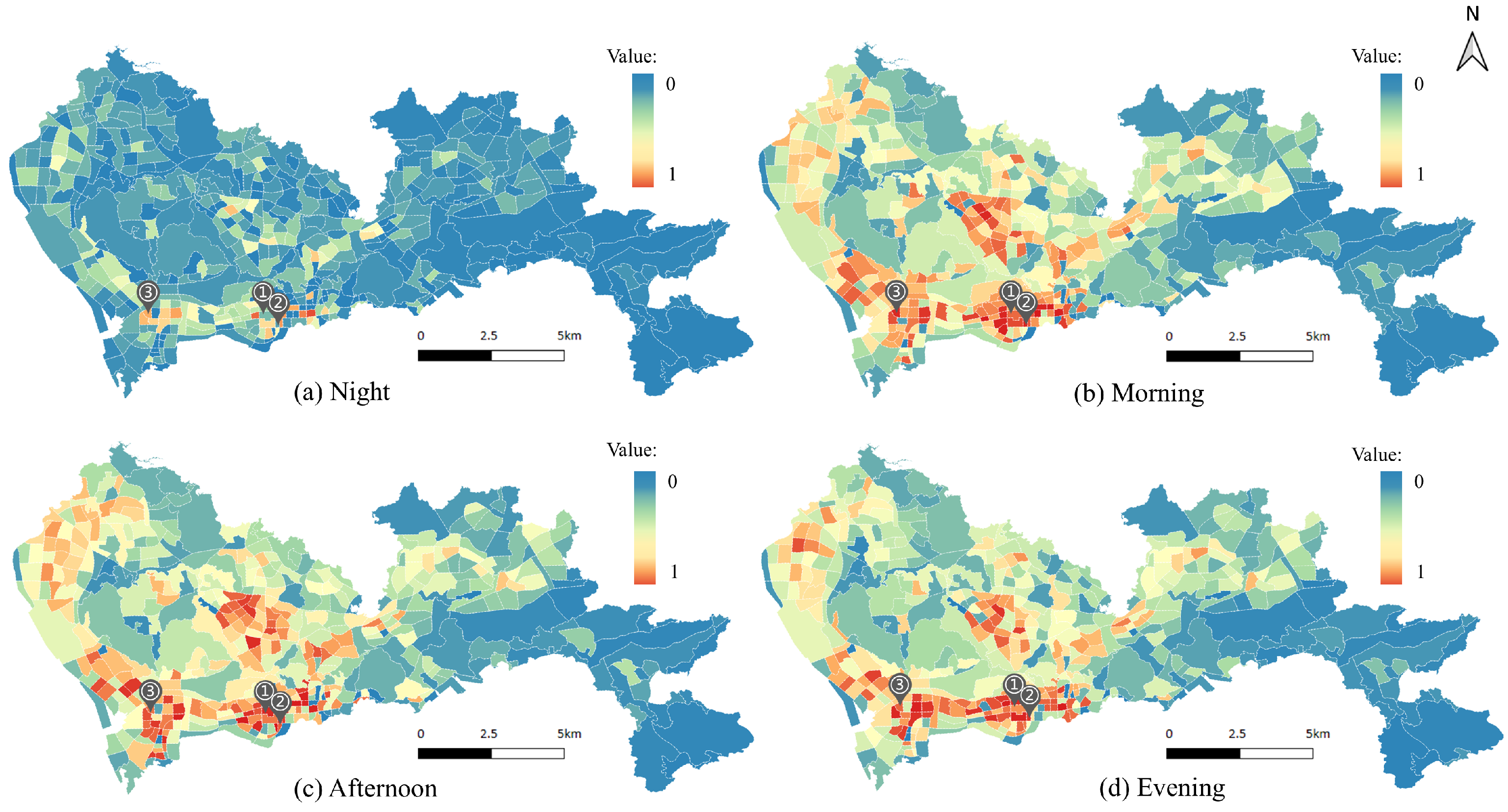
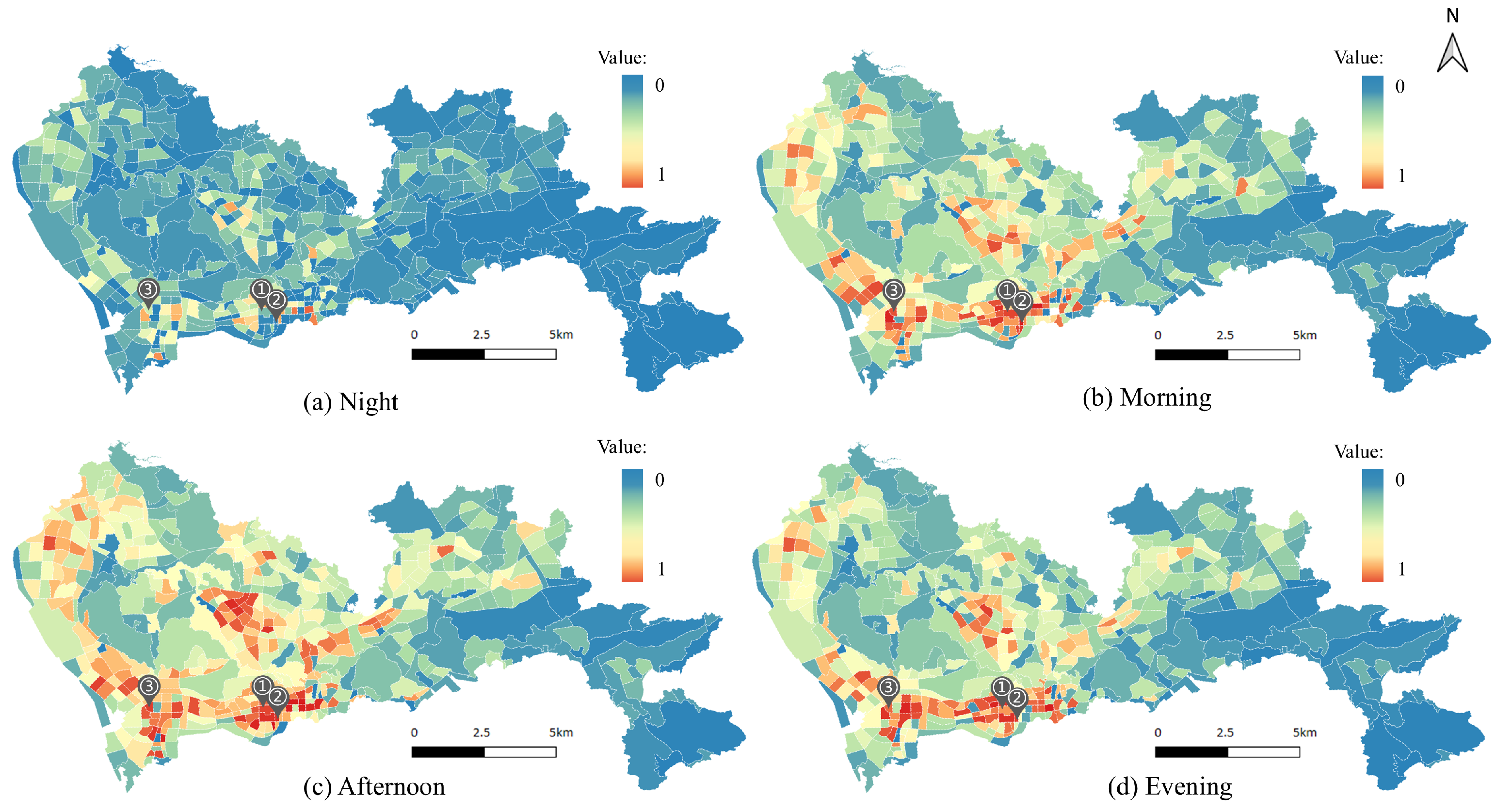
- RQ 2: What distinct spatiotemporal patterns of urban vitality emerge in Shenzhen during weekdays and weekends, and at different times of the day?
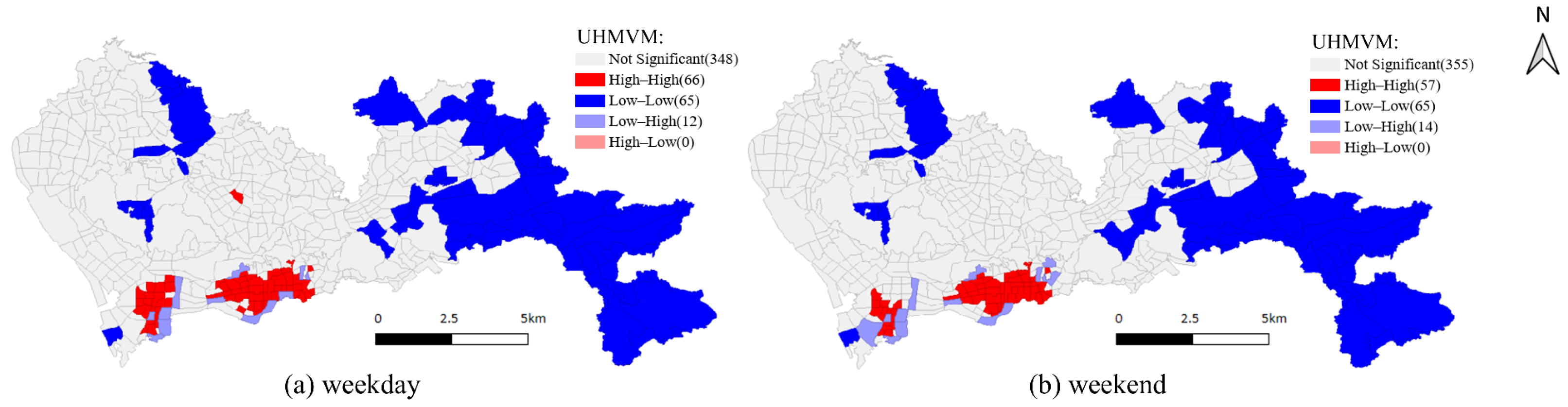
- RQ 3: What areas exhibit significant clustering of high or low vitality, and how do these patterns change over time?
- RQ 4: How do socioeconomic, built environment, and urban landscape factors jointly explain the observed variation in vitality, and what local or nonlinear effects can be identified through advanced modeling techniques?
2. Related Work
2.1. Urban Vitality and Measurement Approaches
2.2. Spatiotemporal Analysis of Urban Vitality
2.3. Influencing Factors of Urban Vitality
3. Study Area and Dataset
3.1. Study Area
3.2. Dataset
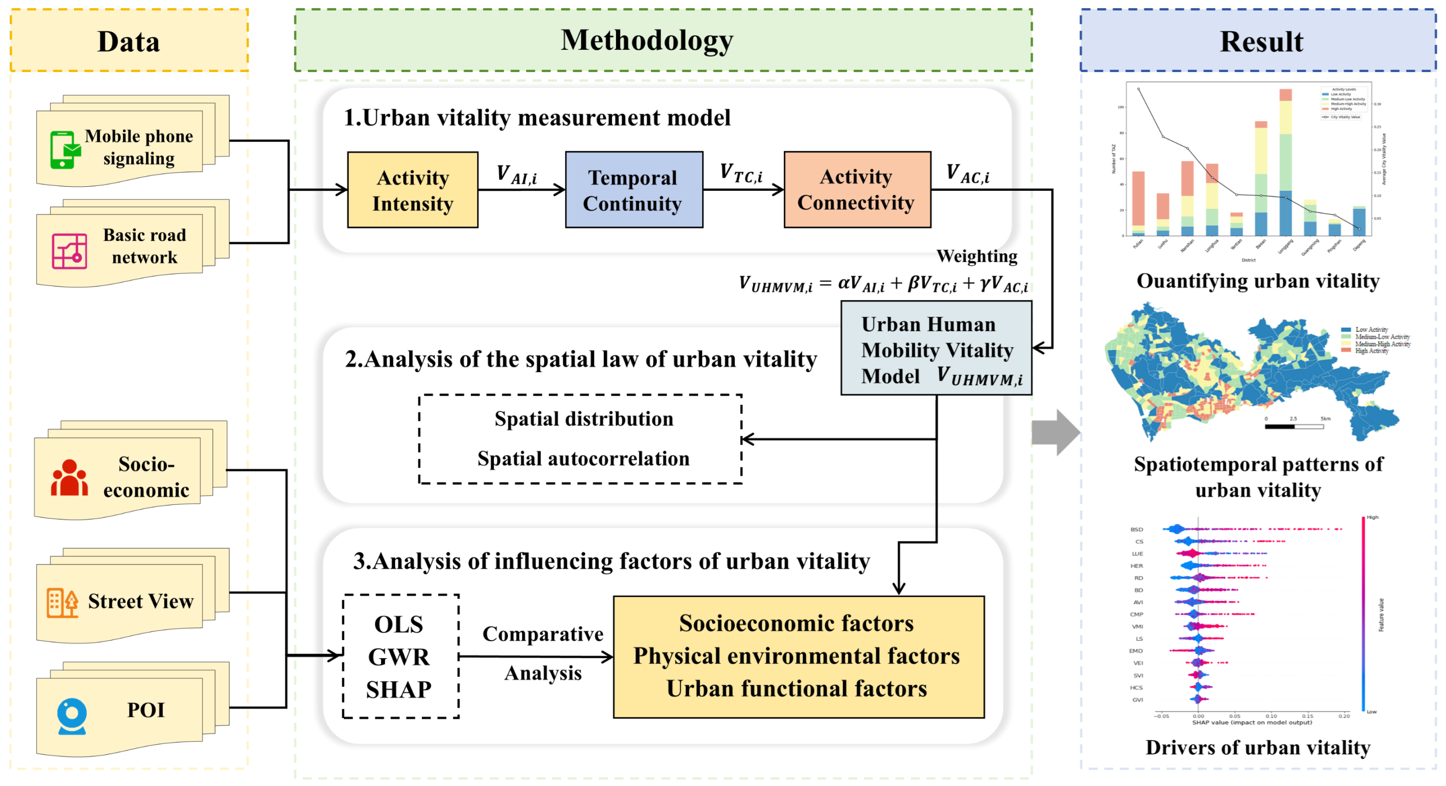
4. Methodology
4.1. Urban Vitality Measure Model
4.1.1. Activity Intensity
4.1.2. Temporal Continuity
4.1.3. Activity Connectivity
4.1.4. Urban Human Mobility Vitality Model
4.2. Vitality Spatial Analysis Model
4.3. Influencing Factors Analysis Model
4.3.1. Indicator System
4.3.2. Linear Regression Model
4.3.3. Geographically Weighted Regression Model
4.3.4. SHAP Model
5. Results
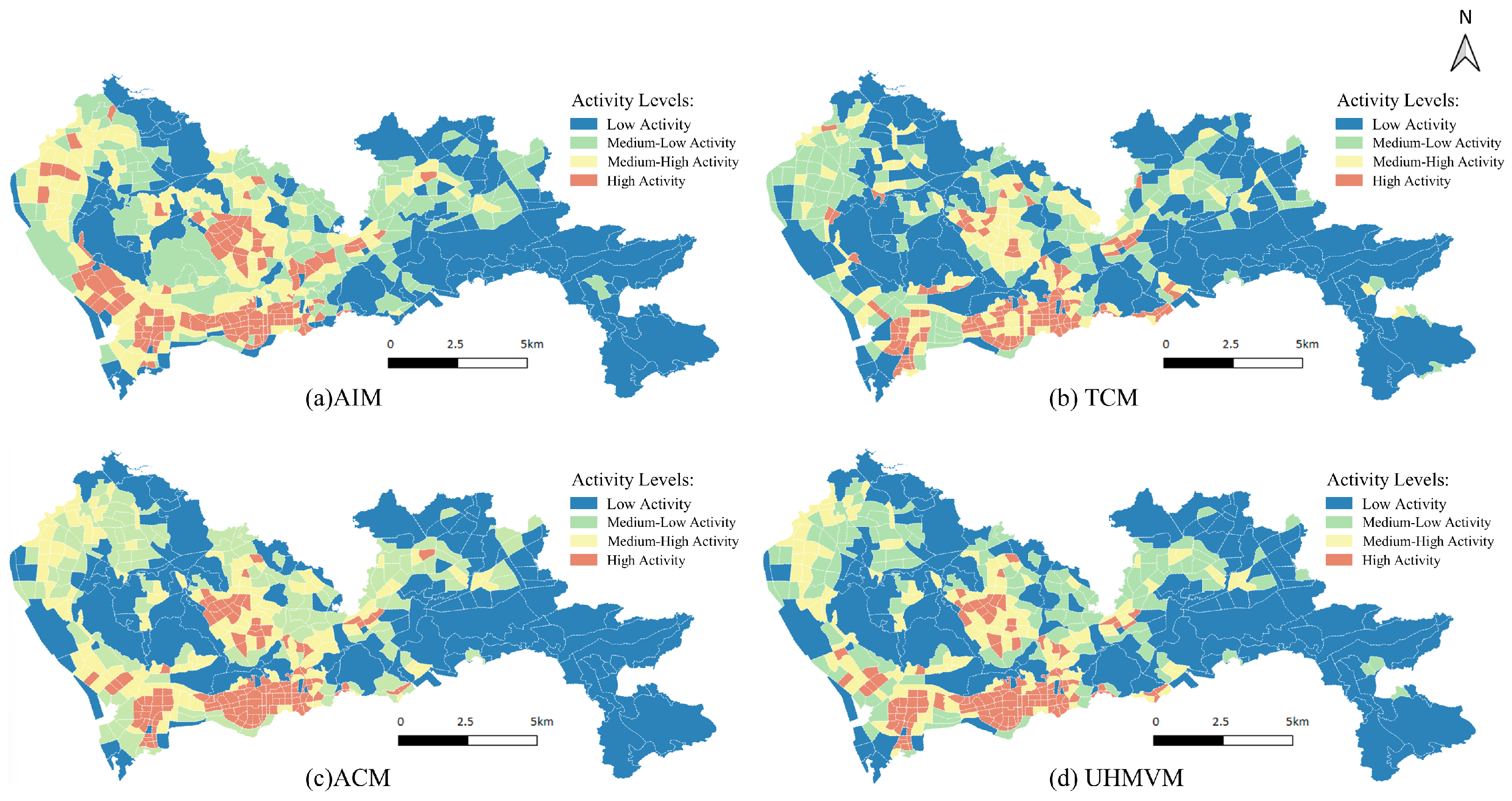
5.1. Urban Vitality Measure and Spatial Distribution
- Low-vitality area: Vitality values in the lowest 25% of all TAZs, indicating relatively weak vitality.
- Medium-low-vitality area: Vitality values between 25% and 50%, representing a moderately low level of vitality.
- Medium-high-vitality area: Vitality values between 50% and 75%, indicating a relatively high level of vitality.
- High-vitality area: Vitality values in the top 25%, showing extremely strong vitality levels.
5.2. Analysis of Spatial Autocorrelation of Urban Vitality
5.3. Analysis of Influencing Factors of Urban Vitality
5.3.1. Regression Analysis
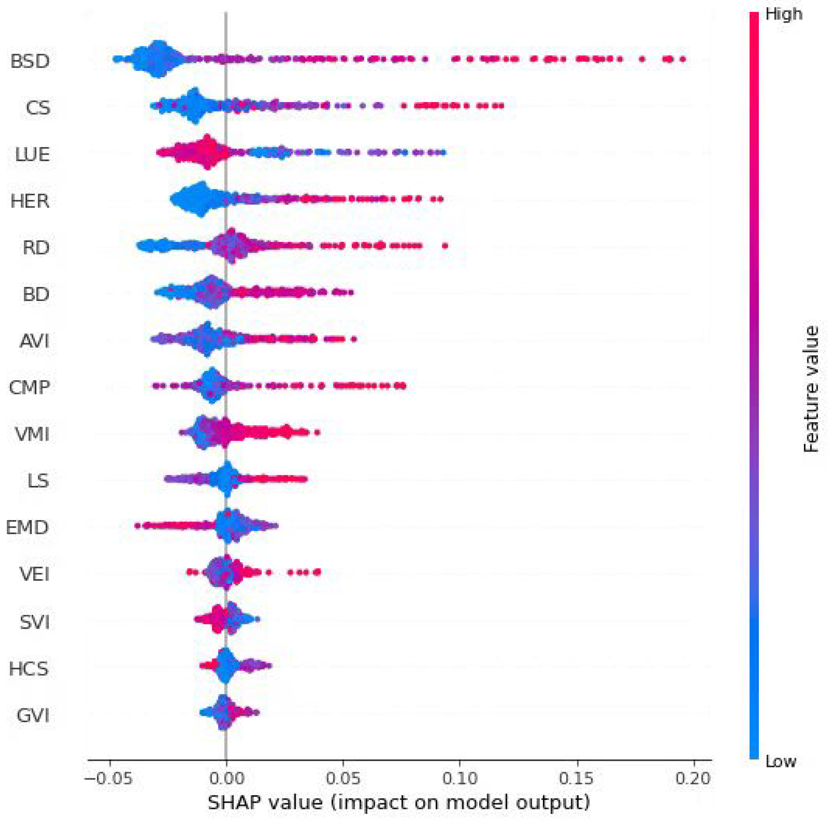
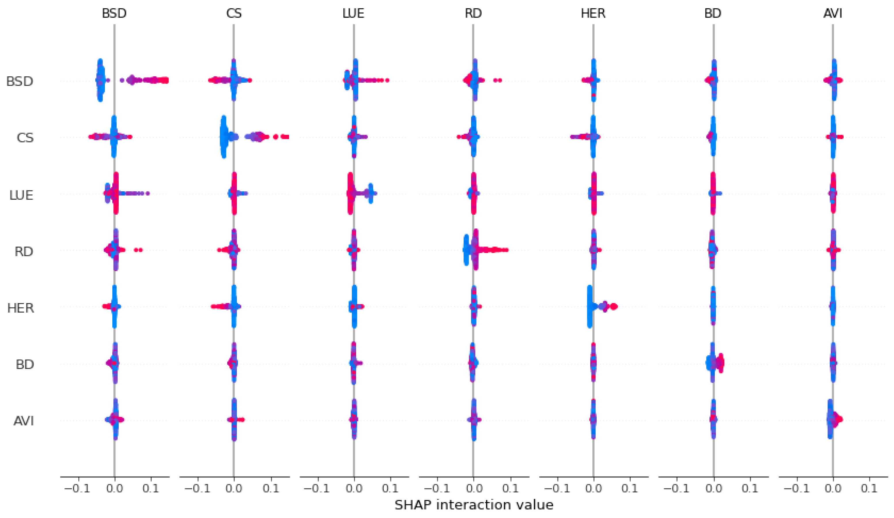
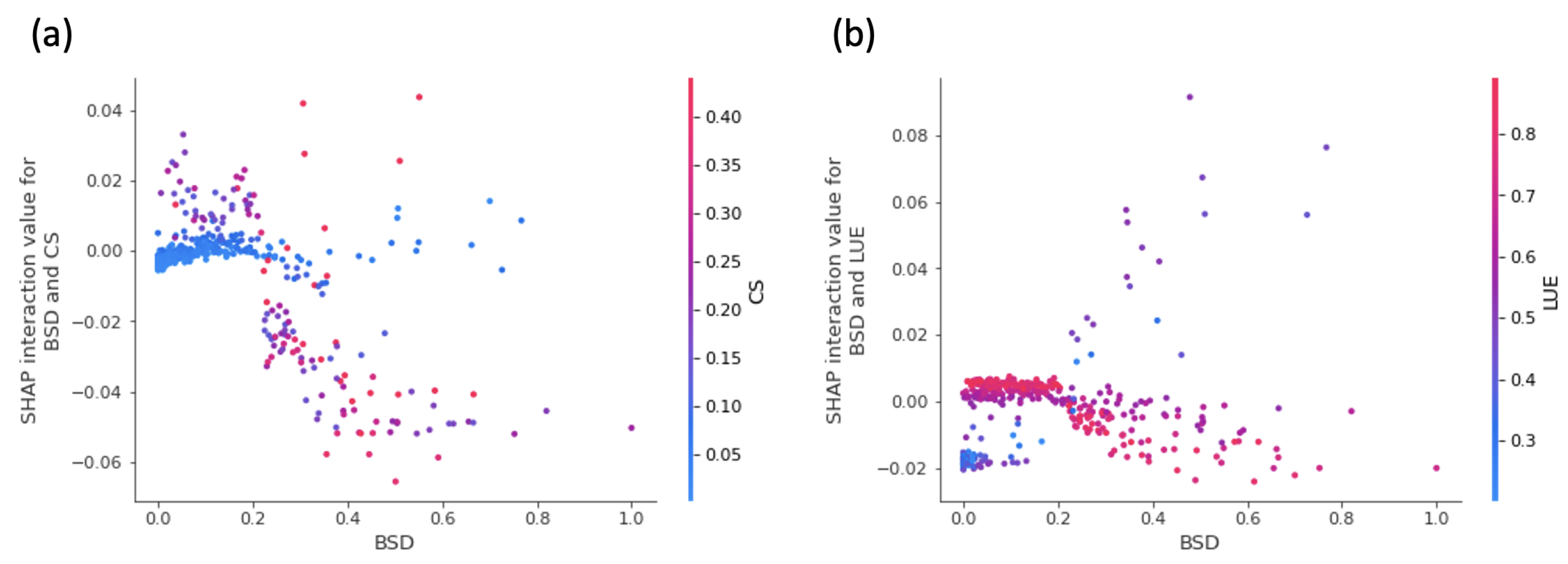
5.3.2. Nonlinear and Feature Importance Analysis
- Socioeconomic Variables: EMD initially boosts vitality at lower-to-moderate levels, reflecting the benefits of economic and social clustering. However, after a threshold, high congestion probably suppresses vibrancy. Similarly, the HER shows a strong positive association up to a point but plateaus once the area is saturated with educated populations.
- Built Environment Variables: RD and BSD both exhibit upward trends in their SHAP values until they reach levels that risk oversaturation or congestion. CS consistently demonstrate a positive relationship, suggesting minimal diminishing returns within the observed range.
- Urban Landscape Variables: Indicators such as the GVI and SVI show more nuanced patterns. At moderate levels, greenery and open skies can support leisure activity, yet exceedingly high values correlate with reduced commercial intensity. This highlights the challenge of balancing environmental quality with robust economic and social functions.
5.3.3. Comparative Analysis of Linear and Nonlinear Models
6. Discussion
6.1. Spatiotemporal Patterns of Urban Vitality
6.2. Drivers of Urban Vitality
6.3. Policy and Planning Imptlications
7. Conclusions
Author Contributions
Funding
Data Availability Statement
Conflicts of Interest
References
- Jacobs, J. Dark Age Ahead: Author of the Death and Life of Great American Cities; Random House of Canada: Toronto, ON, Canada, 2010. [Google Scholar]
- Kim, Y.L. Urban Vitality Measurement Through Big Data and Internet of Things Technologies. ISPRS Int. J. Geo-Inf. 2025, 14, 14. [Google Scholar] [CrossRef]
- Liu, S.; Ge, J.; Ye, X.; Wu, C.; Bai, M. Urban vitality assessment at the neighborhood scale with geo-data: A review toward implementation. J. Geogr. Sci. 2023, 33, 1482–1504. [Google Scholar] [CrossRef]
- Zhao, T.; Liang, X.; Tu, W.; Huang, Z.; Biljecki, F. Sensing urban soundscapes from street view imagery. Comput. Environ. Urban Syst. 2023, 99, 101915. [Google Scholar] [CrossRef]
- Liang, X.; Zhao, T.; Biljecki, F. Revealing spatio-temporal evolution of urban visual environments with street view imagery. Landsc. Urban Plan. 2023, 237, 104802. [Google Scholar] [CrossRef]
- Lan, F.; Gong, X.; Da, H.; Wen, H. How do population inflow and social infrastructure affect urban vitality? Evidence from 35 large-and medium-sized cities in China. Cities 2020, 100, 102454. [Google Scholar] [CrossRef]
- Jacobs, J. The Life and Death of Great American Cities; Random House: New York, NY, USA, 1961. [Google Scholar]
- Montgomery, J. Making a city: Urbanity, vitality and urban design. J. Urban Des. 1998, 3, 93–116. [Google Scholar] [CrossRef]
- Chhetri, P.; Stimson, R.J.; Western, J. Modelling the factors of neighbourhood attractiveness reflected in residential location decision choices. Stud. Reg. Sci. 2006, 36, 393–417. [Google Scholar] [CrossRef]
- Yue, W.; Chen, Y.; Zhang, Q.; Liu, Y. Spatial explicit assessment of urban vitality using multi-source data: A case of Shanghai, China. Sustainability 2019, 11, 638. [Google Scholar] [CrossRef]
- Jalaladdini, S.; Oktay, D. Urban public spaces and vitality: A socio-spatial analysis in the streets of Cypriot towns. Procedia-Soc. Behav. Sci. 2012, 35, 664–674. [Google Scholar] [CrossRef]
- Zarin, S.Z.; Niroomand, M.; Heidari, A.A. Physical and social aspects of vitality case study: Traditional street and modern street in Tehran. Procedia-Soc. Behav. Sci. 2015, 170, 659–668. [Google Scholar] [CrossRef]
- Lyu, G.; Angkawisittpan, N.; Fu, X.; Sonasang, S. Investigating the relationship between built environment and urban vitality using big data. Sci. Rep. 2025, 15, 579. [Google Scholar] [CrossRef]
- Liu, S.; Zhang, L.; Long, Y.; Long, Y.; Xu, M. A new urban vitality analysis and evaluation framework based on human activity modeling using multi-source big data. ISPRS Int. J. Geo-Inf. 2020, 9, 617. [Google Scholar] [CrossRef]
- Wu, C.; Ye, X.; Ren, F.; Du, Q. Check-in behaviour and spatio-temporal vibrancy: An exploratory analysis in Shenzhen, China. Cities 2018, 77, 104–116. [Google Scholar] [CrossRef]
- Kim, Y.L. Seoul’s Wi-Fi hotspots: Wi-Fi access points as an indicator of urban vitality. Comput. Environ. Urban Syst. 2018, 72, 13–24. [Google Scholar] [CrossRef]
- Zeng, C.; Song, Y.; He, Q.; Shen, F. Spatially explicit assessment on urban vitality: Case studies in Chicago and Wuhan. Sustain. Cities Soc. 2018, 40, 296–306. [Google Scholar]
- Xia, C.; Yeh, A.G.O.; Zhang, A. Analyzing spatial relationships between urban land use intensity and urban vitality at street block level: A case study of five Chinese megacities. Landsc. Urban Plan. 2020, 193, 103669. [Google Scholar] [CrossRef]
- He, Q.; He, W.; Song, Y.; Wu, J.; Yin, C.; Mou, Y. The impact of urban growth patterns on urban vitality in newly built-up areas based on an association rules analysis using geographical ‘big data’. Land Use Policy 2018, 78, 726–738. [Google Scholar] [CrossRef]
- Liu, D.; Shi, Y. The influence mechanism of urban spatial structure on urban vitality based on geographic big data: A case study in downtown Shanghai. Buildings 2022, 12, 569. [Google Scholar] [CrossRef]
- Li, Q.; Cui, C.; Liu, F.; Wu, Q.; Run, Y.; Han, Z. Multidimensional urban vitality on streets: Spatial patterns and influence factor identification using multisource urban data. ISPRS Int. J. Geo-Inf. 2021, 11, 2. [Google Scholar] [CrossRef]
- Lee, S.h.; Kang, J.E. Impact of particulate matter and urban spatial characteristics on urban vitality using spatiotemporal big data. Cities 2022, 131, 104030. [Google Scholar] [CrossRef]
- Xia, X.; Zhang, Y.; Zhang, Y.; Rao, T. The spatial pattern and influence mechanism of urban vitality: A case study of Changsha, China. Front. Environ. Sci. 2022, 10, 942577. [Google Scholar] [CrossRef]
- Anselin, L. Local Indicators of Spatial Association—LISA. Geogr. Anal. 1995, 27, 93–115. [Google Scholar] [CrossRef]
- Li, X.; Li, Y.; Jia, T.; Zhou, L.; Hijazi, I.H. The six dimensions of built environment on urban vitality: Fusion evidence from multi-source data. Cities 2022, 121, 103482. [Google Scholar] [CrossRef]
- Chen, Y.; Yu, B.; Shu, B.; Yang, L.; Wang, R. Exploring the spatiotemporal patterns and correlates of urban vitality: Temporal and spatial heterogeneity. Sustain. Cities Soc. 2023, 91, 104440. [Google Scholar] [CrossRef]
- Wu, C.; Zhao, M.; Ye, Y. Measuring urban nighttime vitality and its relationship with urban spatial structure: A data-driven approach. Environ. Plan. B Urban Anal. City Sci. 2023, 50, 130–145. [Google Scholar] [CrossRef]
- Zeng, Z.; Li, Y.; Tang, H. Multidimensional Spatial Driving Factors of Urban Vitality Evolution at the Subdistrict Scale of Changsha City, China, Based on the Time Series of Human Activities. Buildings 2023, 13, 2448. [Google Scholar] [CrossRef]
- Yue, Y.; Zhuang, Y.; Yeh, A.; Xie, J.Y.; Ma, C.L.; Li, Q.Q. Measurements of POI-based mixed use and their relationships with neighbourhood vibrancy. Int. J. Geogr. Inf. Sci. 2017, 31, 658–675. [Google Scholar] [CrossRef]
- Tu, W.; Zhu, T.; Xia, J.; Zhou, Y.; Lai, Y.; Jiang, J.; Li, Q. Portraying the spatial dynamics of urban vibrancy using multisource urban big data. Comput. Environ. Urban Syst. 2020, 80, 101428. [Google Scholar] [CrossRef]
- Lin, J.; Zhuang, Y.; Zhao, Y.; Li, H.; He, X.; Lu, S. Measuring the non-linear relationship between three-dimensional built environment and urban vitality based on a random forest model. Int. J. Environ. Res. Public Health 2022, 20, 734. [Google Scholar] [CrossRef]
- Wu, W.; Niu, X. Influence of built environment on urban vitality: Case study of Shanghai using mobile phone location data. J. Urban Plan. Dev. 2019, 145, 04019007. [Google Scholar] [CrossRef]
- Ye, Y.; Li, D.; Liu, X. How block density and typology affect urban vitality: An exploratory analysis in Shenzhen, China. Urban Geogr. 2018, 39, 631–652. [Google Scholar]
- Zhang, A.; Li, W.; Wu, J.; Lin, J.; Chu, J.; Xia, C. How can the urban landscape affect urban vitality at the street block level? A case study of 15 metropolises in China. Environ. Plan. B Urban Anal. City Sci. 2021, 48, 1245–1262. [Google Scholar]
- Xia, C.; Zhang, A.; Yeh, A.G. The varying relationships between multidimensional urban form and urban vitality in Chinese megacities: Insights from a comparative analysis. Ann. Am. Assoc. Geogr. 2022, 112, 141–166. [Google Scholar]
- Chen, M.; Cai, Y.; Guo, S.; Sun, R.; Song, Y.; Shen, X. Evaluating implied urban nature vitality in San Francisco: An interdisciplinary approach combining census data, street view images, and social media analysis. Urban For. Urban Green. 2024, 95, 128289. [Google Scholar]
- Li, M.; Liu, J.; Lin, Y.; Xiao, L.; Zhou, J. Revitalizing historic districts: Identifying built environment predictors for street vibrancy based on urban sensor data. Cities 2021, 117, 103305. [Google Scholar]
- Chen, Z.; Dong, B.; Pei, Q.; Zhang, Z. The impacts of urban vitality and urban density on innovation: Evidence from China’s Greater Bay Area. Habitat Int. 2022, 119, 102490. [Google Scholar]
- Lu, S.; Shi, C.; Yang, X. Impacts of built environment on urban vitality: Regression analyses of Beijing and Chengdu, China. Int. J. Environ. Res. Public Health 2019, 16, 4592. [Google Scholar] [CrossRef] [PubMed]
- Doan, Q.C.; Ma, J.; Chen, S.; Zhang, X. Nonlinear and threshold effects of the built environment, road vehicles and air pollution on urban vitality. Landsc. Urban Plan. 2025, 253, 105204. [Google Scholar]
- Ling, Z.; Zheng, X.; Chen, Y.; Qian, Q.; Zheng, Z.; Meng, X.; Kuang, J.; Chen, J.; Yang, N.; Shi, X. The Nonlinear Relationship and Synergistic Effects between Built Environment and Urban Vitality at the Neighborhood Scale: A Case Study of Guangzhou’s Central Urban Area. Remote Sens. 2024, 16, 2826. [Google Scholar] [CrossRef]
- Miller, H.J.; Shaw, S.L. Geographic Information Systems for Transportation: Principles and Applications; Oxford University Press: New York, NY, USA, 2001. [Google Scholar]
- Yang, B.; Tian, Y.; Wang, J.; Hu, X.; An, S. How to improve urban transportation planning in big data era? A practice in the study of traffic analysis zone delineation. Transp. Policy 2022, 127, 1–14. [Google Scholar]
- Zhang, Y.; Song, Y.; Zhang, W.; Wang, X. Working and residential segregation of migrants in Longgang City, China: A mobile phone data-based analysis. Cities 2024, 144, 104625. [Google Scholar]
- Gonzalez, M.C.; Hidalgo, C.A.; Barabasi, A.L. Understanding individual human mobility patterns. Nature 2008, 453, 779–782. [Google Scholar] [CrossRef]
- Wills, R. Google’s PageRank-the math behind the search engine. Math. Intell. 2006, 28, 6–11. [Google Scholar] [CrossRef]
- Jia, C.; Du, Y.; Wang, S.; Bai, T.; Fei, T. Measuring the vibrancy of urban neighborhoods using mobile phone data with an improved PageRank algorithm. Trans. GIS 2019, 23, 241–258. [Google Scholar]
- Zhang, L.; Chen, P.; Hui, F. Refining the accessibility evaluation of urban green spaces with multiple sources of mobility data: A case study in Shenzhen, China. Urban For. Urban Green. 2022, 70, 127550. [Google Scholar]
- Li, S.; Chen, P.; Hui, F.; Gong, M. Evaluating urban vitality and resilience under the influence of the COVID-19 pandemic from a mobility perspective: A case study in Shenzhen, China. J. Transp. Geogr. 2024, 117, 103886. [Google Scholar]
- Getis, A. A history of the concept of spatial autocorrelation: A geographer’s perspective. Geogr. Anal. 2008, 40, 297–309. [Google Scholar] [CrossRef]
- Ord, J.K.; Getis, A. Local spatial autocorrelation statistics: Distributional issues and an application. Geogr. Anal. 1995, 27, 286–306. [Google Scholar] [CrossRef]
- Glaeser, E.L.; Gottlieb, J.D. Urban resurgence and the consumer city. Urban Stud. 2006, 43, 1275–1299. [Google Scholar] [CrossRef]
- Ewing, R.; Cervero, R. Travel and the Built Environment: A Meta-Analysis. J. Am. Plan. Assoc. 2010, 76, 265–294. [Google Scholar]
- Yi, S.; Li, X.; Wang, R.; Guo, Z.; Dong, X.; Liu, Y.; Xu, Q. Interpretable spatial machine learning insights into urban sanitation challenges: A case study of human feces distribution in San Francisco. Sustain. Cities Soc. 2024, 113, 105695. [Google Scholar]
- Liu, C.; Wu, X.; Wang, L. Analysis on land ecological security change and affect factors using RS and GWR in the Danjiangkou Reservoir area, China. Appl. Geogr. 2019, 105, 1–14. [Google Scholar] [CrossRef]
- Harris, P.; Fotheringham, A.S.; Juggins, S. Robust geographically weighted regression: A technique for quantifying spatial relationships between freshwater acidification critical loads and catchment attributes. Ann. Assoc. Am. Geogr. 2010, 100, 286–306. [Google Scholar] [CrossRef]
- Zhou, Q.; Wang, C.; Fang, S. Application of geographically weighted regression (GWR) in the analysis of the cause of haze pollution in China. Atmos. Pollut. Res. 2019, 10, 835–846. [Google Scholar] [CrossRef]
- Kumar, I.E.; Venkatasubramanian, S.; Scheidegger, C.; Friedler, S. Problems with Shapley-value-based explanations as feature importance measures. In Proceedings of the International Conference on Machine Learning, PMLR, Virtual, 13–18 July 2020; pp. 5491–5500. [Google Scholar]
- Lundberg, S.M.; Lee, S.I. A unified approach to interpreting model predictions. Adv. Neural Inf. Process. Syst. 2017, 30, 4765–4774. [Google Scholar]
- Li, X.; Kozlowski, M.; Salih, S.A.; Ismail, S.B. Evaluating the Vitality of Urban Public Spaces: Perspectives on Crowd Activity and Built Environment. Archnet-IJAR Int. J. Archit. Res. 2024. ahead-of-print. [Google Scholar] [CrossRef]
- Fang, C.; He, S.; Wang, L. Spatial characterization of urban vitality and the association with various street network metrics from the multi-scalar perspective. Front. Public Health 2021, 9, 677910. [Google Scholar] [CrossRef]
- Malizia, E.; Chen, Y. The economic growth and development outcomes related to vibrancy: An empirical analysis of major employment centers in large US cities. Econ. Dev. Q. 2019, 33, 255–266. [Google Scholar] [CrossRef]
- Chen, C.; Wang, J.; Li, D.; Sun, X.; Zhang, J.; Yang, C.; Zhang, B. Unraveling nonlinear effects of environment features on green view index using multiple data sources and explainable machine learning. Sci. Rep. 2024, 14, 30189. [Google Scholar] [CrossRef]
- Qin, J.; Feng, Y.; Sheng, Y.; Huang, Y.; Zhang, F.; Zhang, K. Evaluation of Pedestrian-Perceived Comfort on Urban Streets Using Multi-Source Data: A Case Study in Nanjing, China. ISPRS Int. J. Geo-Inf. 2025, 14, 63. [Google Scholar] [CrossRef]
- Kåresdotter, E.; Page, J.; Mörtberg, U.; Näsström, H.; Kalantari, Z. First mile/last mile problems in smart and sustainable cities: A case study in Stockholm County. J. Urban Technol. 2022, 29, 115–137. [Google Scholar] [CrossRef]
- Qiao, Y.K.; Peng, F.L.; Dong, Y.H.; Lu, C.F. Planning an adaptive reuse development of underutilized urban underground infrastructures: A case study of Qingdao, China. Undergr. Space 2024, 14, 18–33. [Google Scholar] [CrossRef]
- Mamajonova, N.; Oydin, M.; Usmonali, T.; Olimjon, A.; Madina, A.; Marg‘uba, M. The role of green spaces in urban planning enhancing sustainability and quality of life. Holders Reason. 2024, 2, 346–358. [Google Scholar]
- Fu, R.; Zhang, X.; Yang, D.; Cai, T.; Zhang, Y. The relationship between urban vibrancy and built environment: An empirical study from an emerging city in an arid region. Int. J. Environ. Res. Public Health 2021, 18, 525. [Google Scholar] [CrossRef]
- Yun, H.J.; Park, M.H. Time–space movement of festival visitors in rural areas using a smart phone application. Asia Pac. J. Tour. Res. 2015, 20, 1246–1265. [Google Scholar] [CrossRef]
- Montgomery, J. Editorial urban vitality and the culture of cities. Plan. Pract. Res. 1995, 10, 101–110. [Google Scholar] [CrossRef]
- Yue, W.; Chen, Y.; Thy, P.T.M.; Fan, P.; Liu, Y.; Zhang, W. Identifying urban vitality in metropolitan areas of developing countries from a comparative perspective: Ho Chi Minh City versus Shanghai. Sustain. Cities Soc. 2021, 65, 102609. [Google Scholar] [CrossRef]


| Item | Source | Description | Quantity |
|---|---|---|---|
| Mobile phone signaling data | China Mobile Communications Group Co., Ltd. (Beijing, China) | Mobile signaling data have the potential to accurately identify the distribution of pedestrian flow, containing information about the movement from one TAZ to another at specific moments. | 854,782 |
| Socioeconomic data | Shenzhen Planning and Natural Resources Bureau Information Center | Social attribute data refer to information that describes the social, economic, and cultural characteristics of specific populations, often used to analyze demographic structures and social behaviors. | 491 |
| Street view data | Baidu Maps | Urban physical environment data are input into deep learning models for semantic segmentation, which filters and reorganizes the data to obtain various elements. | 491 |
| POI data (points of interest) | Amap (Gaode Map) | The dataset of 23 categories of POI is filtered and reorganized. | 491 |
| Original_TAZ | Destination_TAZ | Time (Hours) | Number_Total |
|---|---|---|---|
| 102 | 102 | 6 | 1 |
| 102 | 102 | 10 | 51 |
| 102 | 102 | 13 | 15 |
| 102 | 104 | 7 | 3 |
| 102 | 104 | 10 | 4 |
| Variable | Abbreviation | Description | Unit |
|---|---|---|---|
| Socioeconomic variables | |||
| Employment density | EMD | Number of employed people per square kilometer | |
| Higher education ratio | HER | Proportion of individuals with higher education per square kilometer | |
| Average income | AVI | Average monthly income in thousands | thousand/month |
| Built environment variables | |||
| Land use entropy | LUE | Measure of diversity in land use types | % |
| Road density | RD | Total length of roads per square kilometer | |
| Bus stop density | BSD | Number of bus stops per square kilometer | |
| Cultural services | CS | Number of cultural service facilities per square kilometer | |
| Life services | LS | Number of life service facilities per square kilometer | |
| Healthcare services | HCS | Number of healthcare service facilities per square kilometer | |
| Companies | CMP | Number of company service facilities per square kilometer | |
| Buildings | BD | Number of building service facilities per square kilometer | |
| Urban landscape | |||
| Green view index | GVI | % | |
| Sky view index | SVI | % | |
| Visual enclosure index | VEI | % | |
| Visual motorization index | VMI | % |
| Model | Weekday | Weekend | ||
|---|---|---|---|---|
| Moran’s I | z-Value | Moran’s I | z-Value | |
| AIM | 0.4621 | 15.00 | 0.4172 | 13.70 |
| TCM | 0.4956 | 16.54 | 0.4934 | 16.39 |
| ACM | 0.5784 | 19.21 | 0.5848 | 19.75 |
| UHMVM | 0.5885 | 19.43 | 0.5739 | 19.78 |
| Variable | OLS | GWR | |||
|---|---|---|---|---|---|
| Coefficient | SE | t-Statistic | Mean Coefficient | Mean SE | |
| EMD | −0.216 | 0.038 | −5.663 | −0.164 | 0.069 |
| HER | 0.247 | 0.046 | 5.413 | 0.172 | 0.085 |
| AVI | 0.014 | 0.040 | 0.342 | 0.028 | 0.071 |
| LUE | −0.074 | 0.021 | −3.450 | −0.068 | 0.037 |
| RD | 0.188 | 0.035 | 5.363 | 0.140 | 0.061 |
| BSD | 0.210 | 0.039 | 5.429 | 0.192 | 0.066 |
| CS | 0.254 | 0.059 | 4.334 | 0.196 | 0.107 |
| LS | 0.067 | 0.098 | 0.688 | 0.097 | 0.190 |
| HCS | −0.050 | 0.071 | −0.715 | −0.018 | 0.129 |
| CMP | 0.198 | 0.086 | 2.293 | 0.226 | 0.163 |
| BD | 0.026 | 0.064 | 0.398 | 0.025 | 0.110 |
| GVI | −3.651 | 2.309 | −1.581 | −2.367 | 4.098 |
| SVI | −2.668 | 1.672 | −1.596 | −1.735 | 2.965 |
| VEI | −1.859 | 1.171 | −1.587 | −1.206 | 2.078 |
| VMI | −1.130 | 0.765 | −1.476 | −0.664 | 1.362 |
| AICc | −964.151 | −993.862 | |||
| R2 | 0.704 | 0.780 | |||
| Adjusted R2 | 0.693 | 0.735 | |||
| Variable | OLS | GWR | |||
|---|---|---|---|---|---|
| Coefficient | SE | t-Statistic | Mean Coefficient | Mean SE | |
| EMD | −0.175 | 0.036 | −4.871 | −0.141 | 0.065 |
| HER | 0.199 | 0.043 | 4.609 | 0.138 | 0.081 |
| AVI | 0.013 | 0.037 | 0.336 | 0.025 | 0.067 |
| LUE | −0.062 | 0.020 | −3.089 | −0.056 | 0.036 |
| RD | 0.160 | 0.033 | 4.836 | 0.121 | 0.058 |
| BSD | 0.196 | 0.036 | 5.393 | 0.179 | 0.062 |
| CS | 0.219 | 0.055 | 3.960 | 0.160 | 0.102 |
| LS | 0.213 | 0.092 | 2.311 | 0.193 | 0.180 |
| HCS | −0.068 | 0.067 | −1.017 | −0.014 | 0.122 |
| CMP | −0.016 | 0.081 | −0.192 | 0.064 | 0.155 |
| BD | 0.057 | 0.061 | 0.946 | 0.049 | 0.105 |
| GVI | −3.046 | 2.178 | −1.398 | −1.787 | 3.888 |
| SVI | −2.224 | 1.577 | −1.410 | −1.313 | 2.813 |
| VEI | −1.552 | 1.105 | −1.404 | −0.915 | 1.971 |
| VMI | −0.942 | 0.722 | −1.305 | −0.495 | 1.292 |
| AICc | −1016.520 | −1,042.553 | |||
| R2 | 0.679 | 0.758 | |||
| Adjusted R2 | 0.667 | 0.709 | |||
Disclaimer/Publisher’s Note: The statements, opinions and data contained in all publications are solely those of the individual author(s) and contributor(s) and not of MDPI and/or the editor(s). MDPI and/or the editor(s) disclaim responsibility for any injury to people or property resulting from any ideas, methods, instructions or products referred to in the content. |
© 2025 by the authors. Published by MDPI on behalf of the International Society for Photogrammetry and Remote Sensing. Licensee MDPI, Basel, Switzerland. This article is an open access article distributed under the terms and conditions of the Creative Commons Attribution (CC BY) license (https://creativecommons.org/licenses/by/4.0/).
Share and Cite
Wu, Y.; Xie, C.; Zhang, A.; Zhao, T.; Cao, J. Spatiotemporal Analysis of Urban Vitality and Its Drivers from a Human Mobility Perspective. ISPRS Int. J. Geo-Inf. 2025, 14, 167. https://doi.org/10.3390/ijgi14040167
Wu Y, Xie C, Zhang A, Zhao T, Cao J. Spatiotemporal Analysis of Urban Vitality and Its Drivers from a Human Mobility Perspective. ISPRS International Journal of Geo-Information. 2025; 14(4):167. https://doi.org/10.3390/ijgi14040167
Chicago/Turabian StyleWu, Youwan, Chenxi Xie, Aiping Zhang, Tianhong Zhao, and Jinzhou Cao. 2025. "Spatiotemporal Analysis of Urban Vitality and Its Drivers from a Human Mobility Perspective" ISPRS International Journal of Geo-Information 14, no. 4: 167. https://doi.org/10.3390/ijgi14040167
APA StyleWu, Y., Xie, C., Zhang, A., Zhao, T., & Cao, J. (2025). Spatiotemporal Analysis of Urban Vitality and Its Drivers from a Human Mobility Perspective. ISPRS International Journal of Geo-Information, 14(4), 167. https://doi.org/10.3390/ijgi14040167