Remotely Sensed Soil Data Analysis Using Artificial Neural Networks: A Case Study of El-Fayoum Depression, Egypt

Abstract

Earth observation and monitoring of soil quality, long term changes of soil characteristics and deterioration processes such as degradation or desertification are among the most important objectives of remote sensing. The georeferenciation of such information contributes to the development and progress of the Digital Earth project in the framework of the information globalization process. Earth observation and soil quality monitoring via remote sensing are mostly based on the use of satellite spectral data. Advanced techniques are available to predict the soil or land use/cover categories from satellite imagery data. Artificial Neural Networks (ANNs) are among the most widely used tools for modeling and prediction purposes in various fields of science. The assessment of satellite image quality and suitability for analysing the soil conditions (e.g., soil classification, land use/cover estimation, etc.) is fundamental. In this paper, methodology for data screening and subsequent application of ANNs in remote sensing is presented. The first stage is achieved via: (i) elimination of outliers, (ii) data pre-processing and (iii) the determination of the number of distinguishable soil “classes” via Eigenvalues Analysis (EA) and Principal Components Analysis (PCA). The next stage of ANNs use consists of: (i) building the training database, (ii) optimization of ANN architecture and database cleaning, and (iii) training and verification of the network. Application of the proposed methodology is shown.

1. Introduction

The concept of globalization is a technological unification of the world leading to a global information society. Such processes require several steps such as the design and development of well-organized infrastructures able to solve global and regional problems [1]. To do this, the informatization and georeferenciation of the world’s knowledge is required. This is the task of the “Digital Earth” project. In this framework, remote sensing and earth observation technologies contribute significantly to the progress of Digital Earth. Among the various tasks and objectives of remote sensing sciences is the monitoring of soil characteristics, deterioration, and use (e.g., cultivation or urbanization). Soil degradation and desertification is a phenomenon that affects many countries, especially those with arid and semiarid regions. Common degradation processes include water stress, soil salinization, forest fires, overgrazing and water erosion, etc. Such processes are often monitored using approaches based on various biophysical and socioeconomic indicators. 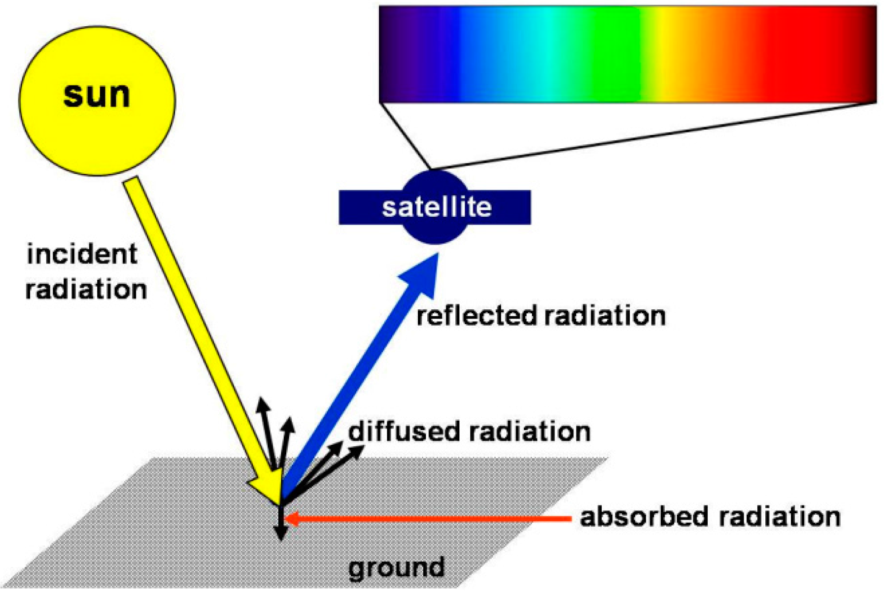The evaluation of such indicators has recently been reported [2]. Other approaches are based on the estimation of the vegetation cover fraction and/or the class of the soil by remote sensing using satellite imagery data (usually reflectance spectra). The scheme of the reflectance data acquisition procedure using a satellite is given in Figure 1.

Figure 1. Scheme of the remote sensing principle. A fraction of sunlight reflected or scattered by the soil is detected at selected wavelengths by the satellite.

Figure 1. Scheme of the remote sensing principle. A fraction of sunlight reflected or scattered by the soil is detected at selected wavelengths by the satellite.

Remote sensing estimation of soil class and land use/cover is a complex process that involves several steps. First, the image of the studied area is recorded by the satellite. The quality of satellite image is given by parameters such as spatial, spectral, radiometric, and temporal resolution. The spatial resolution is related to the dimensions of the pixels in a raster image. The pixel corresponds usually to area with dimensions ranging from 1 to 1000 meters. The spectral resolution refers to the wavelength width of the detected frequency bands. The radiometric resolution indicates the ability of an imaging system to discriminate slight differences in the energy of the detected radiation. The temporal resolution is gathered from the frequency of flyover by the satellite.

Over the studied area, m sampling points are chosen either randomly or using a grid. Soil samples are then collected from the sampling points and classified according to the results of chemical and morphological analysis (Figure 2).

Figure 2. Example of random distribution of 15 sampling points over the studied area. From each sampling point, a soil sample is collected. The class of the collected soil samples is determined by means of chemical and morphological analysis.

Figure 2. Example of random distribution of 15 sampling points over the studied area. From each sampling point, a soil sample is collected. The class of the collected soil samples is determined by means of chemical and morphological analysis.

A table of reflectance spectra of the collected soil samples and their corresponding class constitutes the “database”. The reflectance spectrum of a soil sample depends mostly on the soil chemical composition. Therefore, the reflectance spectra of soils belonging to different classes are expected to be different. Unfortunately, the mathematical law expressing the relation between the reflectance spectrum and the chemical composition of the soil is not known. However, the data in the database contain information that can be used to build an empirical model of the spectrum-soil relationship. The process that leads to obtaining such empirical relation is called “modeling”. The model allows the prediction of the soil class using the reflectance data for arbitrary pixels of the satellite image in places where no sampling and chemical analysis were done. In this way, a map representing the distribution of the various soil classes over the studied area is obtained.

Various mathematical methods are available for the modeling. The choice of the method depends upon the complexity of the data to be modeled. Non-linear methods offer the flexibility required to model complex data structures. Methods based on artificial neural networks are among the most powerful and widespread [3,4]. The application of ANNs in science and technology is quite extensive in various branches of chemistry, physics, biology, social sciences, and economy and they cover classification, modeling, pattern recognition purposes, etc. For example, ANNs are used in chemical kinetics [5], prediction of the behavior of industrial reactors [6], modeling kinetics of drug release [7], prediction of optimal composition of multidrug mixtures [8], optimization of electrophoretic methods [9], classification of agricultural products such as onion varieties [10], and even insect species determination [11,12]. Application of ANNs in medical diagnosis has recently been reviewed [13]. In general, very diverse data such as classification of biological objects, chemical kinetic data, or even clinical parameters can be handled in essentially the same way. Selected examples of ANNs applications in remote sensing are: water quality monitoring [14], estimation of evapotranspiration [15], derivation of ocean color products [16], mapping fractional snow cover [17], prediction of soil organic matter [18], spatial assessment of air temperature [19], mapping contrasting tillage practices [20], classification of soil texture [21] prediction of productive fossil localities [22], sub-pixel mapping and sub-pixel sharpening [23], etc. Often, ANNs are used even when some basic conditions for their use are not fulfilled.

The aim of this work is to present the general philosophy and fundamental methodological steps that should be followed, namely in the evaluation of satellite spectral data using ANNs for soil classification purposes. In particular, the importance of the preliminary data exploration use (data screening) by Eigenvalues Analysis (EA) and Principal Components Analysis (PCA) is stressed. The proposed methodology is exemplified to the evaluation of satellite data concerning El-Fayoum area in Egypt and the results of each step are commented on.

2. The Study Area

El-Fayoum depression is a Governorate located 90 km southwest of Cairo (Figure 3) and characterized by temperate climatic conditions. The total area of the depression is 6068.70 km²; the land use in this area includes only 1849.64 km² (i.e., 30.48% of the total area). The agricultural land in the depression is 1609.34 km². El-Fayoum is connected to the Nile Valley by the Hawara area, where a canal, called Bahr Yousef, is transporting the Nile water. The depression is distinguished by its long history, extending back millions of years, having importance in the emerging Ancient Egyptian, Greek, Roman, Coptic and Islamic eras. It is the only Egyptian Governorate where a salt lake (i.e., Qaroun Lake), vegetation, and desert with their diverse features and unique combination exist. The climatic data of El-Fayoum district indicate that the total rainfall does not exceed 7.2 mm/year and the mean minimum and maximum annual temperatures are 14.5 and 31.0 °C, respectively. The evaporation rates are coinciding with temperatures, where the lowest evaporation rate (1.9 mm/day) was recorded in January while the highest one (7.3 mm/day) was recorded in June [24]. According to the aridity index classes [25], the depression is classified as territory under arid climatic conditions.

The depression has a particular nature, differing from Upper Egypt and the Delta and Oases regions as well. The differences are not limited to agriculture. They extend to geographical and topographical features, as the environment varies between agricultural, desert and coastal areas. The El-Fayoum depression has been formed as a result of basin subsidence, relative to the Nile River, permitting it to break through and to flood the area. This led to the formation of a thick fertile alluvium [26]. The main identified landforms in El-Fayoum depression are fans, recent and old lake terraces, depressions, plains, and basins [27]. With the present regime of practiced flooding and rising of water level in the Qaroun Lake, surrounding arable land would be in danger of salinization and water logging.

Figure 3. Location map of the (a) El-Fayoum depression and (b) satellite image (Landsat ETM 2011).

Figure 3. Location map of the (a) El-Fayoum depression and (b) satellite image (Landsat ETM 2011).

3. Satellite Data

In this study, satellite Digital Number (DN) values of the pixels representing soil sampling sites were used out of different spectral bands which include the seven LANDSAT images (bands 1–5, 7) and three SPOT ones (bands 1, 2 and 3). Wavelengths and spatial resolution of different spectral bands are shown in Table 1.

Table 1. Wavelengths and spatial resolution of satellite spectral bands used.

	Spectral Band	Wavelength (μm)	Resolution (m)
LANDSAT	1	0.45–0.52	30
	2	0.52–0.60	30
	3	0.63–0.69	30
	4	0.77–0.90	30
	5	1.55–1.75	30
	7	2.09–2.35	30
SPOT	1 (green)	0.50–0.59	10
	2 (red)	0.61–0.68	10
	3 (NIR)	0.79–0.89	10

Table 1. Wavelengths and spatial resolution of satellite spectral bands used.

	Spectral Band	Wavelength (μm)	Resolution (m)
LANDSAT	1	0.45–0.52	30
	2	0.52–0.60	30
	3	0.63–0.69	30
	4	0.77–0.90	30
	5	1.55–1.75	30
	7	2.09–2.35	30
SPOT	1 (green)	0.50–0.59	10
	2 (red)	0.61–0.68	10
	3 (NIR)	0.79–0.89	10

4. Software and Computation

All calculations were performed on a standard PC x86 running Microsoft Windows XP Home Edition as operating system. Statistical data processing and analysis were performed using STATISTICA 10 (StatSoft. Inc. 1984–2011, Tulsa, USA). ANN computation was carried out using Trajan Neural Network Simulator, Release 3.0 D (Trajan Software Ltd. 1996–1998, Durham, UK).

5. Preliminary Data Analysis

As outlined in the Introduction, the database is used to build an empirical model by which the class of a soil can be predicted correctly from reflectance data. This can be achieved only if the data in the database contain the information that is able to distinguish samples belonging to different soil classes. Preliminary data analysis by EA allows researchers to estimate the number of distinguishable soil classes while PCA enables data compression and visualization.

5.1. Organization of Experimental Data

For each of the m soil samples collected over the studied area, the value of reflectance intensity is recorded at n wavelengths by the satellite. Data are organized in a matrix X with dimensions m × n. Therefore, the elements of the i-th row of the matrix X represent the reflectance spectrum of the i-th soil sample. Further discussion concerns the analysis of the data in the matrix X.

5.2. Data Pre-Processing

Pre-processing of data in the matrix X consists of: (i) data inspection to search for missing values and (ii) mathematical transformation of data. Various methods such as data smoothing [28] or iterative algorithms [29,30] are available to replace missing values with suitable estimates. Common data transformation includes either column centering or standardization or normalization [31,32]. In this work, data were autoscaled (i.e., centering around column means and scaled by column standard deviations).

5.3. Eigenvalues Analysis

Let us consider a matrix X with m rows and n columns containing error-free data. The column standardized matrix Z is calculated as:

$$Z=\left(X-1_m{\overline{X}}_n^{\text{T}}\right)S_n^{-1}$$

(1)

where 1_m is a vector of length m with all elements equal to one, ${\overline{X}}_n^{\text{T}}$ is the transpose of the vector ${\overline{X}}_n$ which elements are the column mean values of X and $S_n^{-1}$ is the diagonal matrix with dimension n × n in which the main diagonal elements are equal to the column standard deviations of data in matrix X. The matrix Z is used to compute the variance-covariance matrix D as:

$$D=Z{Z}^{\text{T}}$$

(2)

The matrix D is symmetric and with dimension m × m. Linear algebra ensures that the variance-covariance matrix is also positive semi-definite and this implies that all its eigenvalues are non-negative. The first step in the analysis of matrix D is the calculation of its eigenvalues λ_i (i = 1,…, m). This can be done using various approaches [32]. On the principal diagonal of matrix D are the column variances of the original matrix Z. Therefore, the trace of D is equal to the total column variance of Z:

$$trace\left(D\right)={\sigma }^2$$

(3)

A property of variance-covariance matrix and its eigenvalues is that:

$$trace\left(D\right)={\displaystyle \sum }_{i=1}^m{\lambda }_i$$

(4)

and, considering Equation (3):

$${\sigma }^2={\displaystyle \sum }_{i=1}^m{\lambda }_i$$

(5)

Therefore, the percent of the total variance “explained” by the i-th eigenvalue is expressed as:

$$\%{\sigma }^2=\frac{{\lambda }_i}{{{\displaystyle \sum }}_{i=1}^m{\lambda }_i}100$$

(6)

The number of non-zero eigenvalues of a matrix is called “rank” r. In general, considering a matrix with dimension m × n:

$$r\le \text{ min}\left\{m,n\right\}$$

(7)

For the matrix D, the non-zero eigenvalues are only the first r, while the remaining ones are all equal to zero. The rank of D is equal to that of the matrix X.

The number of non-zero eigenvalues (or rank) is interpreted as the number of “factors” responsible for variance in the data. In the case of reflectance data of soils, the rank r of the data matrix X can be interpreted as the number of “distinguishable” soil classes.

Up to now, a matrix X with error-free data has been considered. However, every measured quantity (such as reflectance values) is subject to measurement errors. The consequence is that errors contribute to the overall variance in data (σ²). Therefore, all eigenvalues of the matrix D result as non-zero and its “apparent” rank is equal to m. The m-r eigenvalues represent variance due to measurement errors. The aim of eigenvalues analysis is to estimate the true rank r of the matrix D. Several criteria are available for this purpose [32,33]. A simple method for the estimation of the true rank of the matrix D recommended in this work is the use of the so-called scree-plot [31]. First of all, the n eigenvalues λ_i of the matrix D are calculated and ordered according to their magnitude. The scree-plot is obtained by plotting the magnitude of eigenvalues λ_i against the corresponding value of i. As the value of i increases, the variance explained by the corresponding i-th eigenvalue decreases. Following this, the tangents to the two branches of the scree-plot are drawn and the value of r is found as the integer number closest to the intersection point coordinate at the x axis (Section 7 “Examples”). The knowledge of r value is of fundamental importance for the next application of modeling techniques (such as ANNs).

5.4. Principal Components Analysis

PCA is a technique of exploratory analysis and dimensionality reduction of multivariate data. The eigenvectors and the corresponding eigenvalues of X are obtained by matrix factorization.

An eigenvector is associated with each eigenvalue that is related to the percent of total variance explained by that eigenvalue. The eigenvectors are called “principal components” (PC) and represent successive orthogonal directions of maximum variance in data. Therefore, the eigenvectors define a new coordinate system (principal factor space) in which both the variables and the samples can be represented. Using the scree-plot or other suitable procedure [32], the rank r of matrix D is estimated. Then, the data can be represented in a reduced r-dimensional factor space.

In general, the data matrix X can be decomposed into eigenvalues and eigenvectors by several methods. Among these, the singular value decomposition (SVD) represents one of the more robust and accurate. The SVD leads to the factorization of the matrix X as:

$$X=U\bullet W\bullet V^{\text{T}}$$

(8)

where U is the matrix of normed scores, W is the diagonal matrix of eigenvalues square roots, and V is the matrix of loadings [31,32].

The matrix E = W² is the diagonal matrix of eigenvalues. The trace of E represents the total variance in data. The importance of the k-th principal component is expressed as percent of explained variance (% var_k) using the k-th eigenvalue (λ_k):

$$\%{\text{var}}_k=\frac{{\lambda }_k}{trace\left(E\right)}$$

(9)

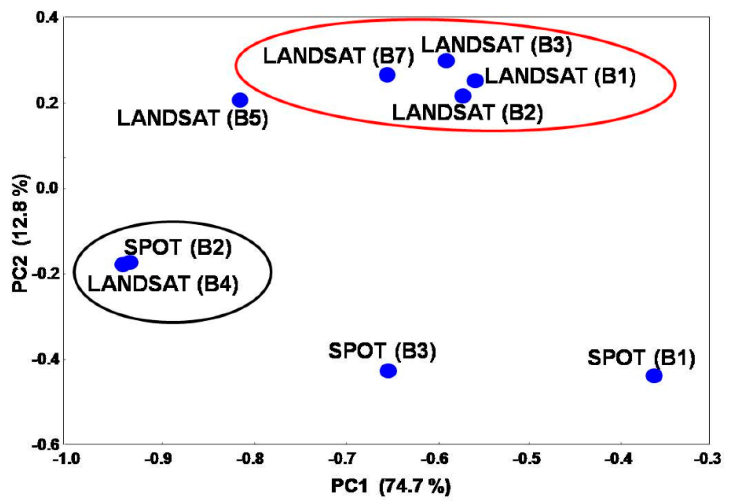
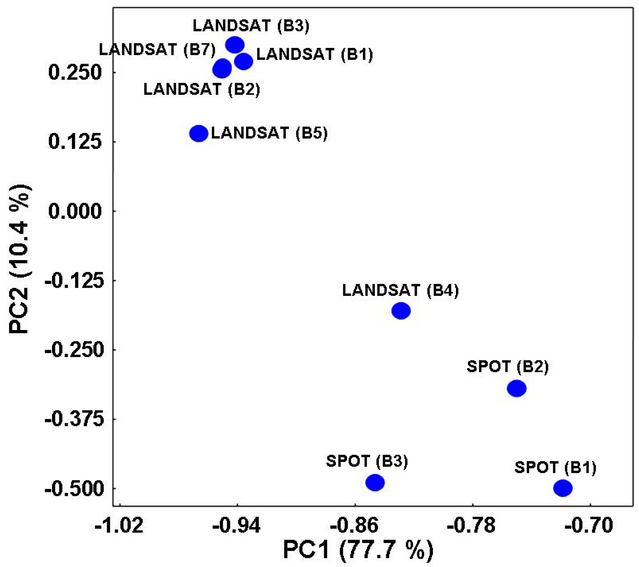
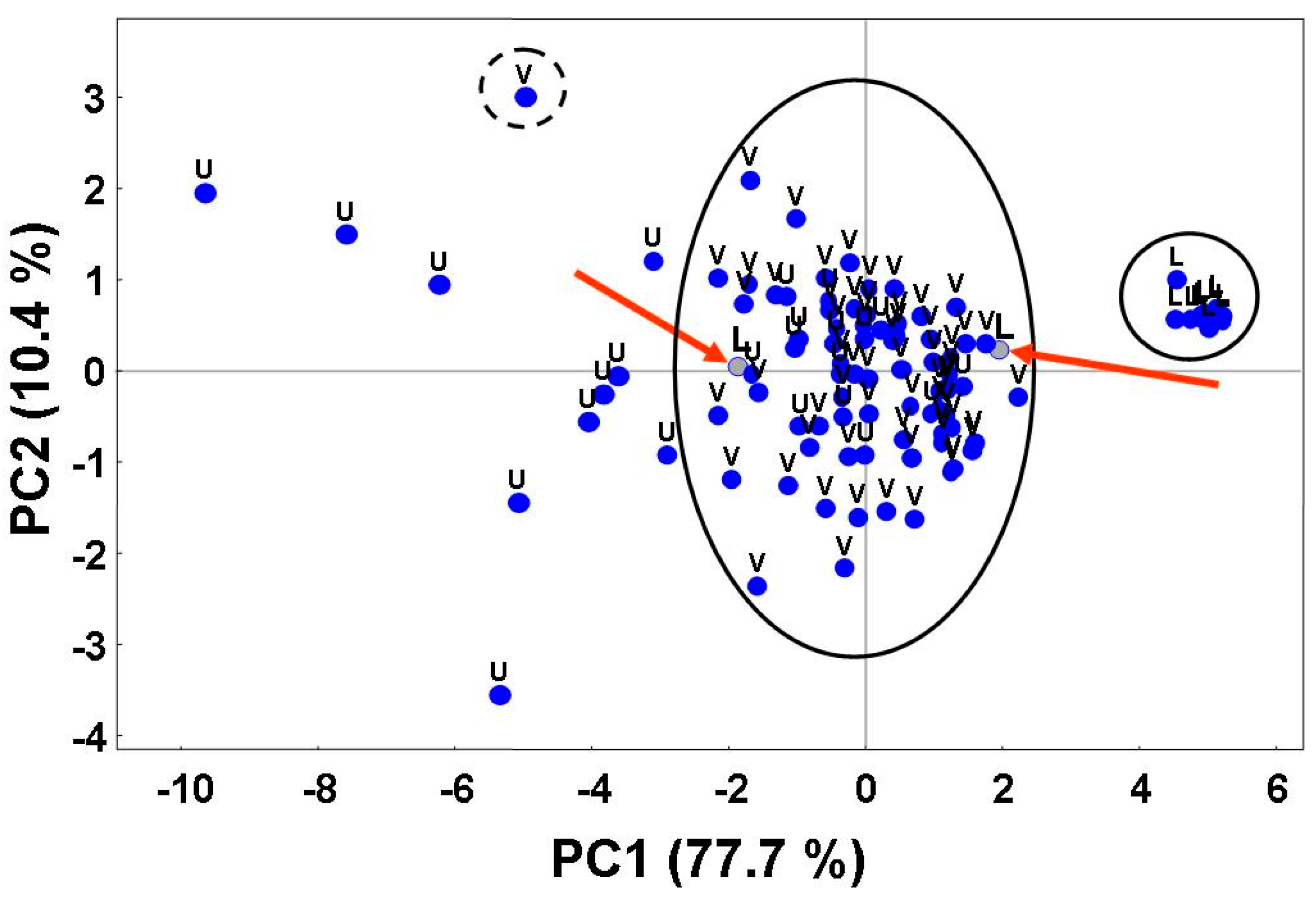
The elements of the k-th column of the matrix V^T represent the coordinates of the variables (satellite spectral bands) on the k-th principal component (loadings). Analogously, the elements of the j-th column of the matrix U represent the coordinates of the soil samples on the j-th principal component (scores). By plotting the columns of U, the distribution of the variables in the reduced r-dimensional principal factor space is visualized (loadings plot). In the same way, the distribution of the samples in the reduced factor space is obtained by plotting the columns of the matrix V^T (scores plot). From such plot, clusters of “similar” samples can be visualized.

6. Artificial Neural Networks

ANNs are mathematical tools that mimic the structure and function of human brain. They are able to perform “learning”, “generalization” and “prediction” tasks. For this reason, ANNs belong to so called methods of artificial intelligence (AI). The network “learns” from a series of “examples” that form the “training database”. An “example” is given by a vector $X_{i,p}=\left(x_{i1},x_{i2},\dots ,x_{ip}\right)$ of inputs and a vector $Y_{i,q}=\left(y_{i1},y_{i2},\dots ,y_{iq}\right)$ of outputs. In the case of soil classification from satellite data, the vectors X_i and Y_i contain the reflectance intensities and the class of the i-th sample, respectively. The objective of the “learning” is to model the unknown relation f between the vectors X_i,p and Y_i,q (Equation (10)):

$$Y_{i,q}=f\left(X_{i,p}\right)$$

(10)

Because of their inherent non-linear nature, ANNs are able to model complex relationships among data. However, PCA remains fundamental to visualize the underlying structure of the data and to get an idea of possible ANN outcomes. Beside the widespread use of multilayer feed-forward neural networks, several other networks including Bayesian, stochastic, recurrent, or fuzzy ones are available. A review of various classes of neural networks can be found elsewhere [34,35].

6.1. Mathematical Background of ANNs

The basic processing unit of a neural network is called a “neuron” (or “node”). The neurons are organized in layers and each neuron in a layer is connected with each neuron in the next layer through a weighted connection. The value of the weight w_ij indicates the strength of the connection between the i-th and the j-th neuron. A neural network is formed by the “input” layer, one or more “hidden” layers, and the “output” layer. The number of hidden layers and that of neurons therein (z) depends on the complexity of the relation f to be modeled (Equation (10)). Therefore, in the first step the network architecture must be optimized. The general scheme of a typical three-layered ANN architecture is given in Figure 4.

Figure 4. Example of three-layered ANN architecture with one hidden layer. The symbol w_ij represents the weight of the connection between the i-th and j-th neuron.

Figure 4. Example of three-layered ANN architecture with one hidden layer. The symbol w_ij represents the weight of the connection between the i-th and j-th neuron.

The data (x_i) received by the input layer are transferred to neurons in the first hidden layer where they are mathematically processed by calculating their weighted sum and adding a “bias” term (θ_j) according to Equation (11):

$$ne{t}_j={\displaystyle \sum }_{i=1}^p{x}_i\times w_{ij}+{\text{θ}}_{\text{j}}\left(j=1,2,\dots ,q\right)$$

(11)

where p and q are defined as stated above. The resulting value of net_j is transformed using a suitable mathematical function (transfer function) and transferred to neurons in the next layer. Various transfer functions are available [35] but the most commonly used is the sigmoid one (Equation (12)):

$$f\left(x\right)=\frac{1}{1+e^{-x}}$$

(12)

At the beginning, random values within the interval [−1,1] are assigned to all the connection weights w_ij. The “learning” is achieved by iterative alteration of the connection weights values (w_ij) according to a given mathematical rule (training algorithm). Various algorithms are available [35,36]. The most common training algorithm is back-propagation (BP) which searches for the values of the weights w_ij that minimize the sum-of-squared residuals (E) calculated as:

$$E=\frac{1}{2}{\displaystyle \sum }_i^p{\displaystyle \sum }_j^q{\left(y_{ij}-y_{ij}^{*}\right)}^2$$

(13)

where y_ij and y_ij^* represent the actual and network j-th output.

The weight change at the k-th epoch on the neurons in a given layer is calculated as:

$$E=-\text{η}\frac{dE}{d{w}_{ij}}+\text{μ Δ}{w}_{ij}^{k-1}$$

(14)

where η is a positive constant called “learning rate”, μ is the “momentum” term, and Δw_ij^k−1 is the change of the weight w_ij from the (k−1)-th epoch. The learning rate controls the speed of the learning while the momentum term stabilizes the process avoiding local minima. Details can be found in monographs [35]. A nice and detailed introduction to ANNs can be found elsewhere [37].

6.2. Optimization of Network Architecture

Optimized network architecture can be obtained using the function given by Equation (13) as a criterion. A widely used approach is to plot the value of E (Equation (13)) as a function of the number z of nodes in the hidden layer (Section 7 “Examples”). The value of E decreases as that of z increases. However, after an optimal value of z, the change in the value of E becomes rather poor.

Usually, the optimal value of z is found from the coordinate of the intersection point of the tangents to the two branches of the plot. Before proceeding with the optimization of ANN architecture, it is advisable to check data in matrix X for the presence of possible outliers using proper statistical tests [31]. The effect of outliers on ANN performance has been reported elsewhere [38]. Methods of outlier detection using ANNs have also been described [39].

6.3. The Verification of the Network

The training process is carried out using the optimal network architecture found until a proper minimum value of E is reached. The “generalization” ability of the network is checked in the so-called “verification” procedure using data not used in the training. A common approach is to use cross-verification by selecting randomly one or more rows of the matrix X for verification and to use the remaining ones for the training. This process is repeated until each row of X has been used for verification at least once. Modern ANN software allows users to perform training and verification simultaneously. After successful training and verification, the network can be used to classify new samples.

6.4. Structure of the Training Database

As stated above, a suitable training database is used to perform ANN training. Such a database is a table (or matrix) of data concerning samples of soil for which the class is known. Each row of the matrix refers to one soil sample. The first n elements of the row are satellite data while the last element is the output (soil class). ANNs require a “sufficient” number of samples for each class, however, such number depends from the complexity of the problem and general rule is not available.

6.5. Data Pre-Processing before ANN Analysis

Data pre-processing is a recommended step before using ANNs. Such step involves mathematical data transformation. Usually, data are scaled within the interval [0,1]. When the matrix X contains missing data, various procedures can be applied such as substitution by data smoothing [28] or removal of the corresponding row and column.

7. Examples

Satellite reflectance data concerning 100 locations randomly chosen in the El-Fayoum area (Figure 5) were recorded at nine wavelengths. The first two examples concern the use of reflectance data for land use/cover estimation. For this purpose, the locations were grouped into “vegetation” (V), “lake” (L) and “urban” (U) classes. The third example concerns the use of reflectance data for soil type classification.

Figure 5. Distribution of 100 locations over the El-Fayoum area (Egypt) for which satellite reflectance data were recorded.

Figure 5. Distribution of 100 locations over the El-Fayoum area (Egypt) for which satellite reflectance data were recorded.

7.1. Distinguishability of “Vegetation” and “Lake” Classes

In this example, reflectance data concerning only: “Vegetation” (V) and “Lake” (L) classes were used. Data were organized in a matrix X with 76 rows and 9 columns.

The eigenvalues of the matrix X were calculated and the number of non-zero eigenvalues (also called structural eigenvalues) was estimated from the scree-plot as shown in Figure 6. As can be seen, two eigenvalues explain 87.54% of the data variance.

7.1.1. Principal Components Analysis

The eigenvectors and the corresponding eigenvalues of the matrix X were computed by SVD. The distribution of the variables and samples in the bi-dimensional principal factor space is given by the loadings and scores plots, respectively. In the loadings plot (Figure 7), two groups of variables are highlighted in ellipses. The smaller is the distance among variables in the loadings plot the higher is their correlation. For example, the small distance between variables SPOT (B2) and LANDSAT (B4) in Figure 7 means that they are highly correlated. Therefore, the spectral bands SPOT (B2) and LANDSAT (B4) are “equivalent” for the distinguishability of V and L classes. The loadings plot is a mean to visualize the extent of correlation among the variables.

Figure 6. Scree-plot obtained for the reflectance data concerning the 76 locations selected in the El-Fayoum Egyptian region. The method of the tangents gives two structural eigenvalues. The percentage of variance in data explained by each eigenvalue is given.

Figure 6. Scree-plot obtained for the reflectance data concerning the 76 locations selected in the El-Fayoum Egyptian region. The method of the tangents gives two structural eigenvalues. The percentage of variance in data explained by each eigenvalue is given.

Figure 7. Representation of the satellite spectral bands (variables) in the reduced bi-dimensional principal factor space. Highly correlated spectral bands are highlighted in ellipses.

Figure 7. Representation of the satellite spectral bands (variables) in the reduced bi-dimensional principal factor space. Highly correlated spectral bands are highlighted in ellipses.

The distribution of the samples in reduced bi-dimensional principal factor space is shown in the scores plot (Figure 8). Clearly, two well-separated clusters of samples are visualized. This result is in agreement with the finding of EA (two structural eigenvalues were found).

Figure 8. Representation of samples in the reduced bi-dimensional principal factor space. Samples belonging to class V are well-separated from those belonging to class V (dotted ellipse).

Figure 8. Representation of samples in the reduced bi-dimensional principal factor space. Samples belonging to class V are well-separated from those belonging to class V (dotted ellipse).

7.1.2. Classification Using ANNs

From the matrix X, the so-called “complete” matrix F was obtained by adding to X a further column containing the class (V, or L) of each sample. The matrix F was used as a training database. In the first step, data were pre-processed by autoscaling (standardization to zero mean and unit standard deviation). In the second step, the optimal neural network architecture was searched for. A network with only one neuron in the hidden layer was found able to correctly classify the samples. This result is due to the fact that clusters in Figure 8 can be separated by a straight line. Therefore, the network performs a simple linear discrimination. The generalization ability of the network was checked by randomly choosing six or more samples at a time to perform cross-verification. It was found that the trained network was always able to predict correctly the class of the sample (100% of correct classification).

7.2. Distinguishability of “Vegetation”, “Lake”, and “Urban” Classes

This example is an extension of the previous one to include also the class “urban” (U) beside the classes V and L. Data were organized in a matrix X with dimensions 100 × 9. The complete matrix F was obtained by adding a further column to X containing the class (V, L or U) of each sample.

7.2.1. Eigenvalues Analysis

As the first step, the eigenvalues of X were calculated. The number of structural eigenvalues was estimated from the scree-plot as shown in Figure 9. In this case, the determination of the number of structural eigenvalues is not straightforward as in the previous case. We know that data were collected for three classes of soil. However, although the first two eigenvalues are quite different from each other, the difference between the second and the third eigenvalue is quite small. This indicates that probably two of the three soil classes are barely distinguishable.

Figure 9. Scree-plot obtained from reflectance data concerning “vegetation”, “lake”, and “urban” classes (El-Fayoum Egyptian region). The number of structural eigenvalues is most probably equal to two.

Figure 9. Scree-plot obtained from reflectance data concerning “vegetation”, “lake”, and “urban” classes (El-Fayoum Egyptian region). The number of structural eigenvalues is most probably equal to two.

7.2.2. Principal Components Analysis

The matrix X was decomposed using the SVD algorithm. The loadings plot (Figure 10) shows the distribution of the spectral bands used in the reduced bi-dimensional principal factor space. The spectral bands LANDSAT (B1-5, 7) are highly correlated.

Figure 10. Loadings plot representing the distribution of the satellite spectral bands (variables) in the reduced bi-dimensional principal factor space. PC1 and PC2 are the first and the second principal component, respectively.

Figure 10. Loadings plot representing the distribution of the satellite spectral bands (variables) in the reduced bi-dimensional principal factor space. PC1 and PC2 are the first and the second principal component, respectively.

The scores plot is shown in Figure 11. Only samples belonging to the L class can be clearly distinguished from the others. This finding is in agreement with the results of EA. As can be seen, there is a partial overlap of the clusters for the classes U and V (highlighted by ellipse in Figure 11). This might mean that several samples represent “green” urban zones. In the same way, the samples belonging to the class L highlighted by red arrows in Figure 11 might be either “outliers” or samples representing “lake” areas where vegetation is abundant. The sample highlighted by the dotted circle in Figure 11 is quite far from the other samples belonging to the V class. However, this does not necessarily mean that the sample in the dotted circle represents an outlier. Its position in the scores plot indicates that it might represent an urban area where vegetation is also present (e.g., a park in a city).

Figure 11. Distribution of samples in the reduced bi-dimensional factor space given by the first and second principal components (PC1 and PC2, respectively). The partial overlap of clusters for samples belonging to the U class with that for samples belonging to the V class is highlighted by the black ellipse. The arrows indicate possible outliers. The doubtful case is highlighted with a dotted circle.

Figure 11. Distribution of samples in the reduced bi-dimensional factor space given by the first and second principal components (PC1 and PC2, respectively). The partial overlap of clusters for samples belonging to the U class with that for samples belonging to the V class is highlighted by the black ellipse. The arrows indicate possible outliers. The doubtful case is highlighted with a dotted circle.

From the results of PCA, it is clear that the reflectance data used contain enough information to discriminate clearly the class “lake” from both “urban” and “vegetation” ones. However, data do not allow complete distinguishability of pure urban and “green” urban areas by PCA. Therefore, we can expect that after removal of the outliers from the database, ANNs can distinguish samples from class L from those belonging to either U or V classes.

7.2.3. Classification Using ANNs

The training database was cleaned from seven outliers as described in Section 6.2 (“Optimization of network architecture”). The plot of E vs. number of neurons in the first hidden layer (z) is shown in Figure 12. The coordinates of the intersection points of the two tangents on the x axis indicates that the minimum number of neurons in the hidden layer to model the data is equal to three. Here, a network with four neurons in the first hidden layer was used.

The “generalization” ability of the trained network was checked by cross-verification using one sample at a time. Such process was repeated until all samples were used at least once. Although PCA was not able to clearly discriminate classes U and V, the percentages of correctly classified samples using ANNs are: 100% (class L), 92% (class V), and 84% (U).

Figure 12. Plot of the sum-of-squared residuals (E) as a function of the number z of neurons in the first hidden layer of the network. The optimal value of z is equal to three.

Figure 12. Plot of the sum-of-squared residuals (E) as a function of the number z of neurons in the first hidden layer of the network. The optimal value of z is equal to three.

7.3. Distinguishability of Soils According to Their Taxonomy

Chemical and morphological analysis of 71 soil samples collected over the El-Fayoum depression area was done and the soils were classified according to the USDA soil taxonomy into the following subgroups: typic haplocalcids, lithic haplocalcids, typic quartzipsamments, typic torripsamments, typic petrogypsids, typic torriorthens, typic haplosalids, vertic torrifluvents, typic torrifluvents, and petrogypsic gypsiorthids. Reflectance data concerning the 71 soil samples were organized in a matrix X with dimensions 71 × 9 and pre-processed as described previously. The number of structural eigenvalues of X was found to be equal to two (94.60% of the total variance). This means that reflectance data in X allow researchers to distinguish only two “groups” of soils. Therefore, the soil samples were classified again according to their suborder in agreement with the USDA soil taxonomy. The new classes so obtained were: fluvents, calcids, salids and psamments (labelled as F, C, S and P, respectively). However, it has been demonstrated that even these four classes cannot be discriminated. It was found that really only the classes “F” and “P” were distinguishable (scores plot given in Figure 13). These results demonstrate the power of data screening. In fact, the eigenvalues analysis is proving that available reflectance data do not contain sufficient information to discriminate all of the four soil suborders. To achieve higher discrimination capability, more spectral bands are needed.

Reflectance data concerning samples belonging only to “F” and “P” classes were used in the ANN classification step. After removing two outliers as marked in Figure 13, neural networks with two neurons in the hidden layer achieved 100% correct classification of soil samples.

Figure 13. Distribution of samples in the reduced bi-dimensional factor space given by the first and second principal components (PC1 and PC2, respectively). The labels “F” and “P” refer to “fluvent” and “psamment” soil classes, respectively. The arrows indicate possible outliers.

Figure 13. Distribution of samples in the reduced bi-dimensional factor space given by the first and second principal components (PC1 and PC2, respectively). The labels “F” and “P” refer to “fluvent” and “psamment” soil classes, respectively. The arrows indicate possible outliers.

8. Conclusions

Remote sensing using satellite spectral data enables efficient monitoring of soil quality to a large extent. ANNs represent powerful tools to estimate soil classes, and the assessment of the suitability of satellite spectral data is a fundamental step.

On the basis of real satellite spectral data, methodology for the purposes of soil classification and land use/cover estimation by artificial neural networks was developed pointing out the main issues that are often overlooked. Eigenvalues analysis and principal components analysis were proven to be powerful means of assessment in advancing the number of distinguishable soil classes and suitability of spectral bands for soil classification. Data screening was shown to be an important prerequisite to improve remotely sensed data analysis using artificial neural networks.

In conclusion, the developed procedure for remotely sensed data screening and their subsequent ANN analysis provides affordable results contributing to the objectives of Digital Earth.

References

1. Konečný, M. The Digital Earth: Spatial data infrastructures from local to global concept. In Towards Digital Earth: Proceedings of the International Symposium on Digital Earth; Science China Press: Beijing, China, 1999; pp. 1–12. [Google Scholar]
2. Kairis, O.; Kosmas, C.; Karavitis, C.; Ritsema, C.; Salvati, L.; Acikalin, S.; Alcalá, M.; Alfama, P.; Atlhopheng, J.; Barrera, J.; et al. Evaluation and selection of indicators for land degradation and desertification monitoring: Types of degradation, causes, and implications for management. Environ. Manag. 2013, 54, 971–982. [Google Scholar]
3. Mas, J.F.; Flores, J.J. The application of artificial neural networks to the analysis of remotely sensed data. Int. J. Remote Sens. 2008, 29, 617–663. [Google Scholar] [CrossRef]
4. Sharma, P.; Mutreja, U. Analysis of satellite images using artificial neural network. Int. J. Soft Comput. Eng. 2013, 2, 276–278. [Google Scholar]
5. Amato, F.; González-Hernández, L.; Havel, J. Artificial neural networks combined with experimental design: A “soft” approach for chemical kinetics. Talanta 2012, 93, 72–78. [Google Scholar] [CrossRef]
6. Molga, E.J.; van Woezik, B.A.A.; Westerterp, K.R. Neural networks for modelling of chemical reaction systems with complex kinetics: Oxidation of 2-octanol with nitric acid. Chem. Eng. Process. 2000, 39, 323–334. [Google Scholar] [CrossRef]
7. Li, Y.; Rauth, A.M.; Wu, X.Y. Prediction of kinetics of doxorubicin release from sulfopropyl dextran ion-exchange microspheres using artificial neural networks. Eur. J. Pharm. Sci. 2005, 24, 401–410. [Google Scholar] [CrossRef]
8. Pivetta, T.; Isaia, F.; Trudu, F.; Pani, A.; Manca, M.; Perra, D; Amato, F; Havel, J. Development and validation of a general approach to predict and quantify the synergism of anti-cancer drugs using experimental design and artificial neural networks. Talanta 2013, 115, 84–93. [Google Scholar] [CrossRef]
9. Havel, J.; Peña, E.M.; Rojas-Hernández, A.; Doucet, J.P.; Panaye, A.J. Neural networks for optimization of high-performance capillary zone electrophoresis methods: A new method using a combination of experimental design and artificial neural networks. J. Chromatogr. A 1998, 793, 317–329. [Google Scholar] [CrossRef]
10. Rodríguez Galdón, B.; Peña-Méndez, E.M.; Havel, J.; Rodríguez Rodríguez, E.M.; Díaz Romero, C. Cluster analysis and artificial neural networks multivariate classification of onion varieties. J. Agric. Food Chem. 2010, 58, 11435–11440. [Google Scholar] [CrossRef]
11. Fedor, P.; Malenovský, I.; Vanhara, J.; Sierka, W.; Havel, J. Thrips (Thysanoptera) identification using artificial neural networks. J. Bull. Entomol. Res. 2008, 98, 437–447. [Google Scholar]
12. Muráriková, N.; Vaňhara, J.; Tóthová, A.; Havel, J. Polyphasic approach applying artificial neural networks, molecular analysis and postabdomen morphology to West Palaearctic Tachina spp. (Diptera, Tachinidae). J. Bull. Entomol. Res. 2011, 101, 165–175. [Google Scholar] [CrossRef]
13. Amato, F.; López, A.; Peña-Méndez, E.M.; Vaňhara, P.; Hampl, A.; Havel, J. Artificial neural networks in medical diagnosis. J. Appl. Biomed. 2013, 11, 47–58. [Google Scholar] [CrossRef]
14. Chebud, Y.; Naja, G.M.; Rivero, R.G.; Melesse, A.M. Water quality monitoring using remote sensing and an artificial neural network. Water Air Soil Pollut. 2012, 223, 4875–4887. [Google Scholar] [CrossRef]
15. Chen, Z.; Shi, R.; Zhang, S. An artificial neural network approach to estimate evapotranspiration from remote sensing and AmeriFlux data. Front. Earth Sci. 2012, 7, 103–111. [Google Scholar] [CrossRef]
16. Ioannou, I.; Gilerson, A.; Gross, B.; Moshary, F.; Ahmed, S. Deriving ocean color products using neural networks. Remote Sens. Environ. 2013, 134, 78–91. [Google Scholar] [CrossRef]
17. Dobreva, I.D.; Klein, A.G. Fractional snow cover mapping through artificial neural network analysis of MODIS surface reflectance. Remote Sens. Environ. 2011, 115, 3355–3366. [Google Scholar] [CrossRef]
18. Atazadeh, I. Biomass and Remote Sensing of Biomass; InTech: Rijeka, Croatia, 2011. [Google Scholar]
19. Aher, P.; Adinarayana, J.; Gorantiwar, S. Remote sensing and artificial neural network in spatial assessment of air temperature in a semi-arid watershed. Int. J. Earth Sci. Eng. 2011, 04, 351–354. [Google Scholar]
20. Sudheer, K.P.; Gowda, P.; Chaubey, I.; Howell, T. Artificial neural network approach for mapping contrasting tillage practices. Remote Sens. 2010, 2, 579–590. [Google Scholar] [CrossRef]
21. Zhai, Y.; Thomasson, J.A.; Boggess, J.E.; Sui, R. Soil texture classification with artificial neural networks operating on remote sensing data. Comput. Electron. Agric. 2006, 54, 53–68. [Google Scholar] [CrossRef]
22. Anemone, R. Finding fossils in new ways: An artificial neural network approach to predicting the location of productive fossil localities. Evol. Anthropol. 2011, 180, 169–180. [Google Scholar] [CrossRef]
23. Mertens, K. Sub-pixel mapping and sub-pixel sharpening using neural network predicted wavelet coefficients. Remote Sens. Environ. 2004, 91, 225–236. [Google Scholar] [CrossRef]
24. Central Laboratory for Agricultural Climate (CLAC). Available online: http://www.clac.edu.eg/ (accessed on 2 January 2014).
25. Hulme, M.; March, R. Global Mean Monthly Humidity Surfaces for 1930-59, 1960-89 and Projected for 2020, UNEP/GEMS/GRID; Climatic Research Unit, University of East Anglia: Norwich, UK, 1990. [Google Scholar]
26. Euroconsult. Environmental Profile, Fayoum Governorate, Egypt; Al-Shorouk Press: Cairo, Egypt, 1992. [Google Scholar]
27. Abo El Enean, S.M. Pedogenesis of El-Fayoum Area. Ph.D. Thesis, Al-Azhar University, Cairo, Egypt, May 1985. [Google Scholar]
28. Kankare, J.J. Computation of equilibrium constants for multicomponent systems from spectrophotometric data. Anal. Chem. 1970, 42, 1322–1326. [Google Scholar] [CrossRef]
29. Walczak, B.; Massart, D.L. Dealing with missing data: Part I. Chemom. Intell. Lab. Syst. 2001, 58, 15–27. [Google Scholar] [CrossRef]
30. Walczak, B.; Massart, D.L. Dealing with missing data: Part II. Chemom. Intell. Lab. Syst. 2001, 58, 29–42. [Google Scholar] [CrossRef]
31. Massart, D.L.; Vandeginste, B.G.M.; Buydens, L.M.C.; de Jong, S.; Lewi, P.J.; Smeyers-Verbeke, J. Handbook of Chemometrics and Qualimetrics; Elsevier Science: Amsterdam, The Netherlands, 1997. [Google Scholar]
32. Malinowski, E.R. Factor Analysis in Chemistry, 3rd ed.; John Wiley & Sons Inc.: New York, NY, USA, 2002. [Google Scholar]
33. Havel, J.; Meloun, M. Multiparametric curve fitting VII—Determination of the number of complex species by factor analysis of potentiometric data. Talanta 1985, 32, 171–175. [Google Scholar] [CrossRef] [PubMed]
34. Aleksander, I.; Morton, H. An Introduction to Neural Computing; International Thomson Computer Press: London, UK, 1995. [Google Scholar]
35. Zupan, J.G.J. Neural Networks in Chemistry and Drug Design, 2nd ed.; Wiley VCH: Weinheim, Germany, 1999. [Google Scholar]
36. Ahmed, F.E. Artificial neural networks for diagnosis and survival prediction in colon cancer. Mol. Cancer 2005, 4, 29. [Google Scholar] [CrossRef] [PubMed]
37. Basheer, I.A.; Hajmeer, M. Artificial neural networks: Fundamentals, computing, design, and application. J. Microbiol. Methods 2000, 43, 3–31. [Google Scholar] [CrossRef] [PubMed]
38. Khamis, A.; Ismail, Z. The effects of outliers data on neural network performance. J. Appl. Sci. 2005, 5, 1394–1398. [Google Scholar]
39. Bullen, R.J.; Cornford, D.; Nabney, I.T. Outlier detection in scatterometer data: Neural network approaches. Neural Netw. 2003, 16, 419–426. [Google Scholar] [CrossRef] [PubMed]