Solar Irradiance Modelling with NASA WW GIS Environment

Abstract

In this work we present preliminary results regarding a proof-of-concept project which aims to provide tools for mapping the amount of solar radiation reaching surfaces of objects, accounting for obstructions between objects themselves. The implementation uses the NASA World Wind development platform (NASA WW) to model the different physical phenomena that participate in the process, from the calculation of the Sun’s position relative to the area that is being considered, to the interaction between atmosphere and solid obstructions, e.g., terrain or buildings. A more complete understanding of the distribution of energy from the Sun illuminating elements on the Earth’s surface adds value to applications ranging from planning the renewable energy potential of an area to ecological analyses.

1. Introduction

NASA World Wind (NASA WW) provides open source client and server technologies, based on open standards, to access models of planet Earth, as well as of other planets. NASA WW is developed using Java programming language and provides a software development kit (SDK) for desktop operating systems and for Android. It implements a virtual globe, which is based on the nominal radius of the Earth and augmented with elevation data to implement a digital terrain elevation model (DTM) from available sources [1,2]. To this date, the main elevation data source is the shuttle radar topography mission (SRTM) which delivers elevation in 90 m cells averaged from the original 30 m data [3]; ad hoc Java classes allow the implementation of specific DTMs in order to provide a more accurate model of earth ground elevation data. The scope of NASA WW is not only to provide means for virtual representation of reality through the web and the media, but also to integrate re-usable functions and modules for scientific modelling and analysis. These can be used without any restrictions by researchers to implement dedicated tools to study the numerous inter-linked dynamics that concur to shape our planet’s ecology. The importance of visual representation of modelled dynamics is just as important as analyzing them, as discussed by [4,5].

Solar energy is intrinsically of primary importance for life, but also is important in terms of its capability as a source of renewable energy in our highly (and increasingly) energy-demanding societies. Technology has advanced dramatically, improving the efficiency of solar cells capturing incoming energy from light [6], and having accurate information on the amount of usable solar energy, is of primary importance. For this reason it is valuable to accurately evaluate the potential amount of average energy reaching the spots where such panels are, or will be, installed. A careful simulation in this sense would allow better planning and optimization and would also reduce expenses and probability of errors. As a matter of fact a significant part of the error budget is due to erroneous panel positioning and orientation, or entirely failing to take into account sources of obstruction, near (e.g., neighboring edifices, trees) or far (e.g., morphology of terrain); repositioning of panels, when possible, is quite expensive.

Of the many aspects that make up our environment, the incoming energy (E) from the Sun is without doubt of primary importance. A broad spectrum of wavelengths reaches the atmosphere with a certain energy content. Recent estimation of the mean value of solar radiation reaching the top of atmosphere (ToA) was carried out by the WRC (World Radiation Center) in Davos–Switzerland, with a value of 1367 W/m². The atmosphere acts as a filter with different degrees of abatement of the energy (i.e., transmissivity of the atmosphere) at different wavelengths (λ) depending on the percentage of distribution of gases, temperature and pressure; see [7] for more details on physical laws regarding this aspect. This energy (which can be expressed as a function of the wavelength, i.e., E = f(λ)) reaches the Earth’s surface and is available for primary processes, i.e., photosynthesis, which is responsible for the primary production in the food-chain and thus is responsible for life itself. Carbon fixing is one very important result of this process and has been a critical topic of investigation in the past years. There are specific features of GIS software to calculate spatial energy intensity, and identify potential sites or land constraints [8], as well as numerous tools for 2-D solar-radiation calculation and many are available online. SOLARFLUX is developed using ARC/INFO version 6.1 (vector-based) and GRID GIS software (raster-based); those modules define the surface topography as a raster-based array (grid) of elevation data [9,10]. Solar Analyst is an extension for ArcGIS Desktop (ESRI^©), in its recent versions to this date (9). It generates an upward-looking hemispherical viewshed, i.e., the angular distribution of sky obstruction calculated for each cell of the input DEM. It then proceeds with overlaying raster information related to Sun and sky conditions at the specified time and day of the year, with allowance for partially obstructed sky sectors [11]. Both modules require spatial analyst extension to ArcGIS. The geographic resources analysis support system (GRASS) GIS open source environment [12] provides the r.sun module implemented using the C language; it calculates the raster map of solar irradiance (for instant time, W/m²) and irradiation (as a daily sum, Wh/m²), considering terrain attributes, i.e., slope, aspect, latitude, and applying a factor parameterizing the attenuation of cloud cover [13,14]. GRASS’s r.sun module is used in the photovoltaic geographical information system (PVGIS) to develop a solar radiation database from climatologic data standardized for Europe and to produce raster maps with a cell resolution of 1 km² [15]. SolarGIS is an online service based on a high resolution climate database, systematically build from satellite and meteorological sources. Derived solar parameters are calculated at a spatial resolution up 80 m using a novel terrain disaggregation method and a DTM derived from SRTM-3 data [16,17]. The Solar Energy Planning system (SEP) is a tool developed to support planning and installation of solar water heating panels, photovoltaic panels, passive solar gain; it is implemented in GIS environment (SEPsis) [18,19]. Specific software developed for estimating the yield of photovoltaic systems including effects from near and far shadowing are PVsyst [20] that uses a meteorological database and isotropic sky model, PV*SOL [21] that offers 2-D and 3-D analysis module.

Several methods have been proposed in the literature that are related to directly or indirectly to the estimation of solar energy incoming towards a surface, but they have not been developed and wrapped in a final user-friendly tool. In [22] a 1 m cell size is used to calculate shadow casted at each pixel/cell in the digital surface model (DSM). The shadow is considered to be a 3-D straight line starting at the pixel, sharing its height and having a constant slope equal to the Sun altitude. The shadow line is interrupted whenever, along the line, a DSM cell presents a height value Z that is higher than the shadow line at that position. The analysis for estimating radiation is an empirical relation between air mass and atmospheric transmittance. SORAM [23] uses anisotropic sky condition in order to calculate direct and diffuse light scattering, integrating values from sunrise to sunset. Values are corrected to account for an inclined plane as well as for shadows projected by surrounding objects. 3D-SOLARIA also uses anisotropic sky with a disadvantage of its approach being its current capability only to work with orthogonal surfaces [24]. An adequate vector-based 3-D GIS for modeling is described in [25]; the calculation procedure is based on the combined vector-voxel (volumetric pixel) approach, applying a shadowing algorithm that accounts for neighboring values and conditions. Speed and performance depend on voxel resolution: at common scales of resolution, buildings can be seen as blocks without roof structures, whereas a very high level of detail is needed to resolve roofs.

In this project, we have started to create a framework in NASA WW for estimating solar irradiance availability at specific moments in time and locations, with areas sampled with grids with specific spatial resolutions, and considering sources of obstructions such as terrain morphology and nearby buildings. A simple and intuitive panel allows users to add simple building models that can be positioned by the user; some parameters can be customized as well, i.e., building basic size, and roof type. The goal of this research is to deliver maps of solar radiation, providing estimates of the energy that will be available over an area.

2. Method

There are many factors which come into play in estimating the amount of incoming solar radiation. First, the geometry of the illumination source and sink has to be modelled, i.e., the Sun position relative to the considered area (in terms of the incidence angle). It is noteworthy that the geometry of the illumination (i.e., the incidence angle) changes continuously following two embedded cycles, with daily and yearly periods, respectively. Then, the influence of the elements along the travel path of the Sun’s rays has to be taken into account: the atmosphere, whose anisotropic model can be found in [26], and solid obstructions as well, due for instance to the terrain morphology (e.g., hills), and to man-made artefacts (e.g., buildings) or natural ones (e.g., trees). Full or partial occlusion decreases the potential amount of solar energy which can reach the surface. The system is developed in Java on top of the NASA WW platform and development environment. The focus of the project is to create a modular system with algorithms for Sun position, the irradiance calculation, 3D modelling of obstructions as well as the output products of the model analysis, which are grids of irradiation values called analytic surfaces (Figure 1).

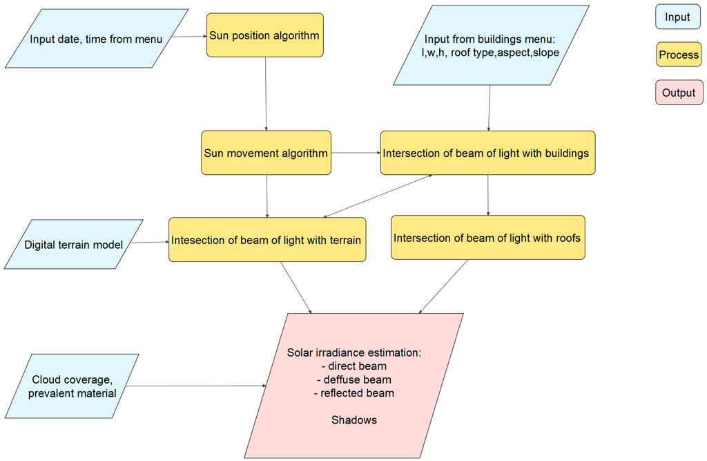
Figure 1. System architecture.

Figure 1. System architecture.

2.1. Sun Position Algorithm

The method for determining Sun position, referred to as the Sun position algorithm (SPA), is taken from [27]. It has an accuracy of 0.0003° and is valid for the next 4000 years. Such characteristics distinguish it from numerous other algorithms in the literature; SPA was chosen for its accuracy and duration in time, as well as the availability of accurate documentation regarding the different parts of the algorithms, which enabled it to be embedded as module in the project. For more documentation on other approaches, [28,29] are important references. The Sun position is fundamental for determining the direction of its beams in relation to the area under examination at a specific time (Figure 2) and to the atmosphere itself. The distance that the energy has to travel through the atmosphere varies depending on the geometry of the travel path, e.g., at sunset the light ray has to travel through ~12 times more atmosphere than at solar noon. At this stage of the project only relatively small areas are considered: according to these operating conditions, the earth curvature can be ignored and the same arrival direction can be considered for all incoming Sun rays, i.e., they have the same incidence angle. Nevertheless, the extension to the general case is immediate, and it will be developed in our future work.

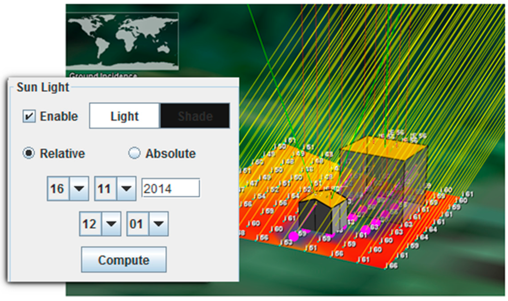
Figure 2. User defines day of the year and time of the day to calculate incidence of Sun rays.

Figure 2. User defines day of the year and time of the day to calculate incidence of Sun rays.

2.2. Atmosphere Model

A model is adopted to estimate the influence of the atmosphere on the energy of the Sun beams over their paths. The main effects are due to absorption and scattering phenomena as described in physics (Rayleigh, Mie and non-selective scattering). Different components are taken into account in the considered model of the atmospheric influence: (e.g., direct and diffuse light reaching the surface [30]). The reflected radiation is available only on non-flat areas, where the incidence angle of Sun rays is greater than zero degrees. Shadow that affects a spot depends on the configuration of the neighboring objects, on its latitude, the time of the day and day of the year. According to the solar irradiance throughout the World Radiation Centre, let G = 1367 (W/m²) be the value of the mean solar irradiance on an area perpendicular to the Sun rays before entering the terrestrial atmosphere at the mean Sun–Earth distance. The variation of the solar irradiance during the year can be calculated as described by [31] using following equations:

$$G_0=G\left(\frac{1+0.033\cos (360n)}{365}\right)$$

(1)

where n is the day index of interest counted from 1st January. Estimation of cloud coverage can be modeled as follows [32]:

$$G_c=G_0(1-0.75{(n/8)}^{3.4})$$

(2)

The direct component of the solar radiation can be computed by means of equations from Equation (3) to Equation (7), whereas the other components of the solar radiation can be derived from the value of the direct one.

$$G_f=t_{f } G_c$$

(3)

where t_f is the transmission coefficient of the direct radiation that depends on the zenith angle z and three parameters a₀, a₁ and a₂ defined as follows:

$$t_f=a_0+{a_1}^{(-\frac{a_2}{cosz})}$$

(4)

$$a_0=0.424-0.0082{\left(6-H\right)}^2$$

(5)

$$a_1=0.5055+0.0060{\left(6.5-H\right)}^2$$

(6)

$$a_2 a2=0.271+0.019{\left(2.5-H\right)}^2$$

(7)

where H is the value of elevation above the sea level, expressed in kilometers (lower than 2.5 km, by assumption).

Equations from Equation (8) to Equation (12) are used to compute the diffuse component, which affects an ideal area located immediately above the surface reached by the direct radiation:

$$G_{dh}=t_d G_f$$

(8)

where t_d is

$$t_d=0.271-0.16t_f$$

(9)

In order to estimate diffuse component G_di it is necessary consider a correction factor, F_hi, which puts the sky virtual surface A_h relative to the ground surface A_i

$$G_{di} A_i =G_{dh} A_h F_{hi}$$

(10)

A_hF_hi = A_iF_ih, Equation (10) can be rewritten as

$$G_{di}=\frac{G_{dh} A_h F_{hi}}{A_i}=\frac{G_{dh}{A}_i{F}_{ih}}{A_i}=G_{dh} F_{ih}$$

(11)

F_ih is the sky portion seen by ground surface; it depends by inclination angle β of the surface with respect to the direction of radiation (Sun rays).

$$G_{di}=G_{dh} \frac{1+\cos \text{β}}{2}$$

(12)

Reflected radiation is computed as described by the following equation:

$$G_{fh}=G_f\cos z$$

(13)

$$G_{ri}={\text{ρ}}_s (G_{fh}+G_{dh}) \frac{1-\cos \text{β}}{2}$$

(14)

where ρ_s is the reflection coefficient of the ground taken from [33]. Table 1 reports a short list of reflection coefficient values for certain common materials.

Table 1. Reflection coefficients ρ from the National agency for new technologies, Energy and sustainable economic development (ENEA).

Material	ρs	Material	ρs
asphalt road	0.10	loam (with clay)	0.14
broad-leaf trees	0.26	roof	0.13
concrete	0.22	snow	0.75
conifers	0.07	stones, gravel	0.20
dark-colored building	0.27	water	0.07
dirt road	0.04	white-colored building	0.60
grass (dry + green)	0.23

Table 1. Reflection coefficients ρ from the National agency for new technologies, Energy and sustainable economic development (ENEA).

Material	ρs	Material	ρs
asphalt road	0.10	loam (with clay)	0.14
broad-leaf trees	0.26	roof	0.13
concrete	0.22	snow	0.75
conifers	0.07	stones, gravel	0.20
dark-colored building	0.27	water	0.07
dirt road	0.04	white-colored building	0.60
grass (dry + green)	0.23

2.3. Building Model

One of the main goals of the developed system is the possibility its utilization to estimate the solar energy that would be potentially available on the surface of a building, not only when already built, but also during or before its construction. In line with this objective, the user can add a virtual representation of the building, setting custom values of length, width and height of the main structure and height of roof’s eaves, as well as specifying the roof typologies (number of sheets) and their slope and orientation.

The characteristics of interest of the building to be constructed are stored in a one-dimensional array, i.e., a vector of values: the building position, its dimensions and orientation. Then, the 3D model is created, in terms of an extruded polygon, using the information from the user-defined model. Finally, the geospatial information is stored in a Java class object.

2.4. Obstructions

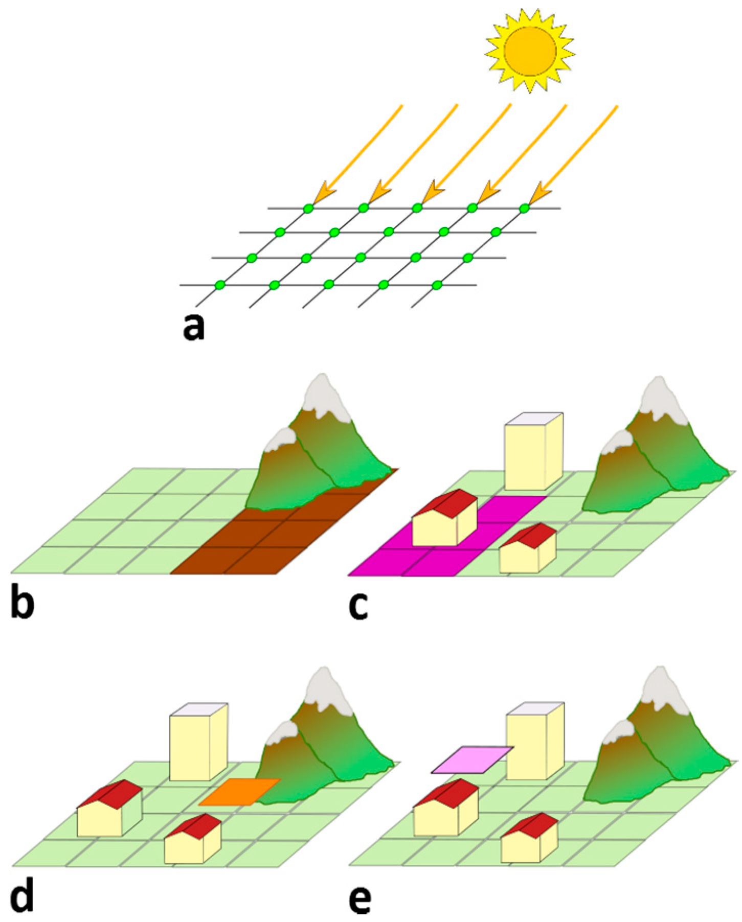
Solid elements can cause partial or full obstruction of the Sun’s energy with respect to the surface considered for calculation. The ray passing from the sun position and a point (i.e., node) on the surface being considered might be intercepted by vegetation, or buildings, or be covered by the skyline due to the terrain’s morphology. The presence of these obstructions is determined by using a specific module in NASA WW. This module considers a layered model of the Earth surface, representing a tessellated terrestrial terrain model and other layers with 3D objects. In this model, the user defines a grid over the bare terrain, at this stage without considering any building. He then creates buildings and obstructions using a specific panel, and drags the buildings into the correct position on the NASA WW globe, thus using all available layers for supporting geo-positioning. The nodes of the grid will be the centers of the final raster map cells. Then, the solar irradiation value is calculated at each node. The process takes into account also of the shadow effects from the node elevation from the ground and of the skyline geometry i.e., morphology of surrounding terrain. The presence of a building over the node is determined by checking if the node position is contained on the building footprint (e.g., a polygon). When a node falls inside a building footprint, then solar irradiance on roof elements of such building is automatically computed. Finally, it computes the shadow effect of the considered building, of other nearby buildings and of skyline shadowing cast on the roof. At the current state of implementation, we handle buildings created by the user with an ad-hoc user interface (Figure 3).

Figure 3. (a) Grid created on terrain; for each point the incidence angle and irradiance values are determined; (b) Shadows due to skyline cast on terrain; (c) Shadows due to buildings cast on terrain; (d) Shadows due to buildings cast on roofs; (e) Shadows due to skyline cast on roofs.

Figure 3. (a) Grid created on terrain; for each point the incidence angle and irradiance values are determined; (b) Shadows due to skyline cast on terrain; (c) Shadows due to buildings cast on terrain; (d) Shadows due to buildings cast on roofs; (e) Shadows due to skyline cast on roofs.

2.5. Final Model

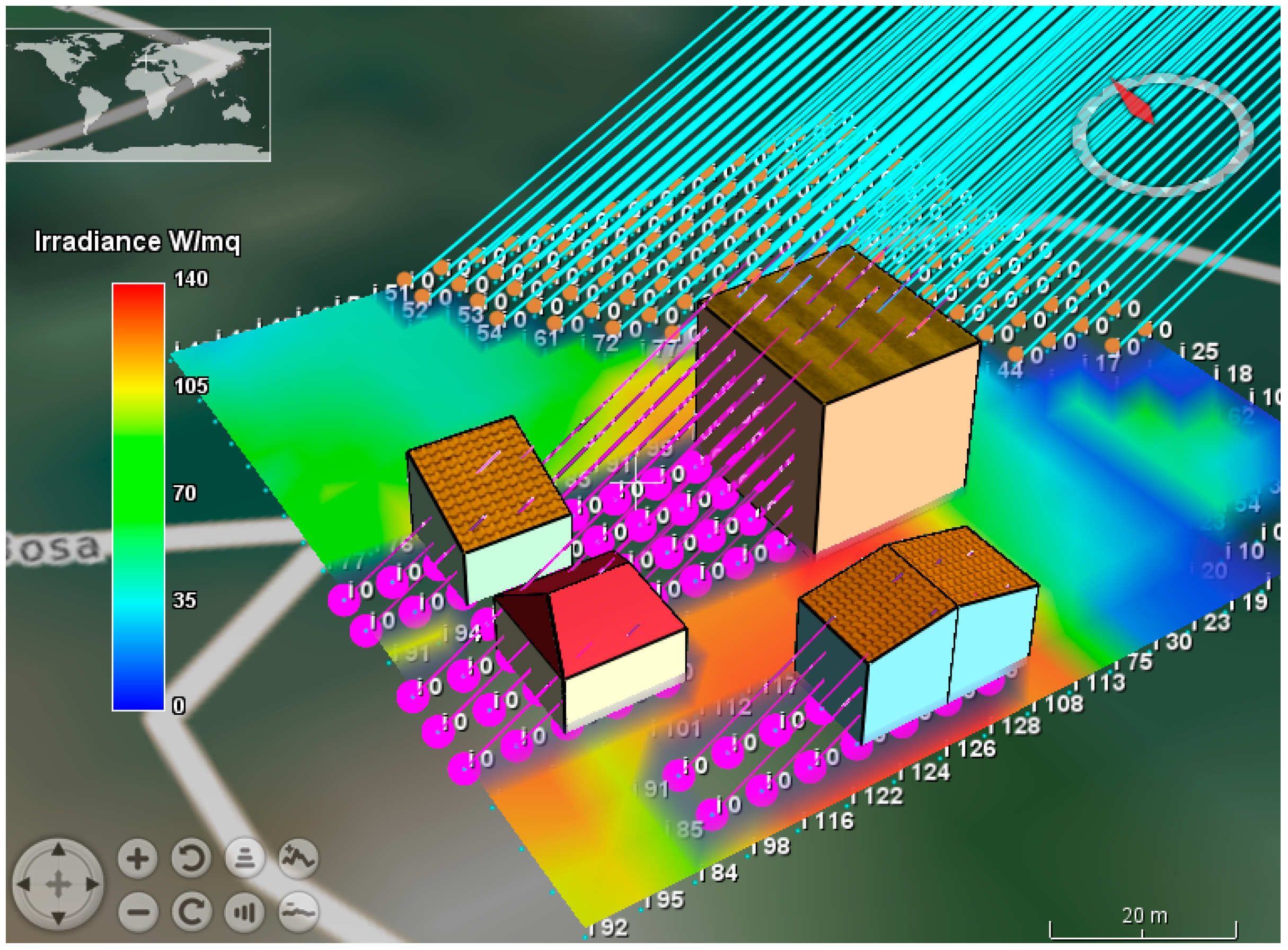
The process is done point-wise over a 2D array representing a projected surface over the Earth’s globe. This is then stored as a grid in NASA WW in terms of an analytical surface object. This necessary simplification can be tuned in terms of grid resolution and size of each cell. The process considers a certain time of day, and also in this case can be reiterated at user-defined time resolutions to calculate a cumulative (day, month, year) amount of energy reaching the surface (Figure 4).

Figure 4. Result of radiation at ground surface considering multiple obstructions. Violet points are shadows created by buildings; brown points are the shadows created by terrain elevation. The numbers on the grid are the values of irradiance.

Figure 4. Result of radiation at ground surface considering multiple obstructions. Violet points are shadows created by buildings; brown points are the shadows created by terrain elevation. The numbers on the grid are the values of irradiance.

3. Experimental Results

At this stage of development of the module the user can define the following parameters:

(i)

a certain time of day and a certain day of year to calculate the sun position;

(ii)

the dimension of the building, i.e., length and width and eaves height;

(iii)

the roof typologies (number of sheets), slope and aspect;

(iv)

a dedicated tool allows to measurement of the size and aspect of building, using available NASA WW layers, i.e., orthophotos or satellite images (Figure 5);

(v)

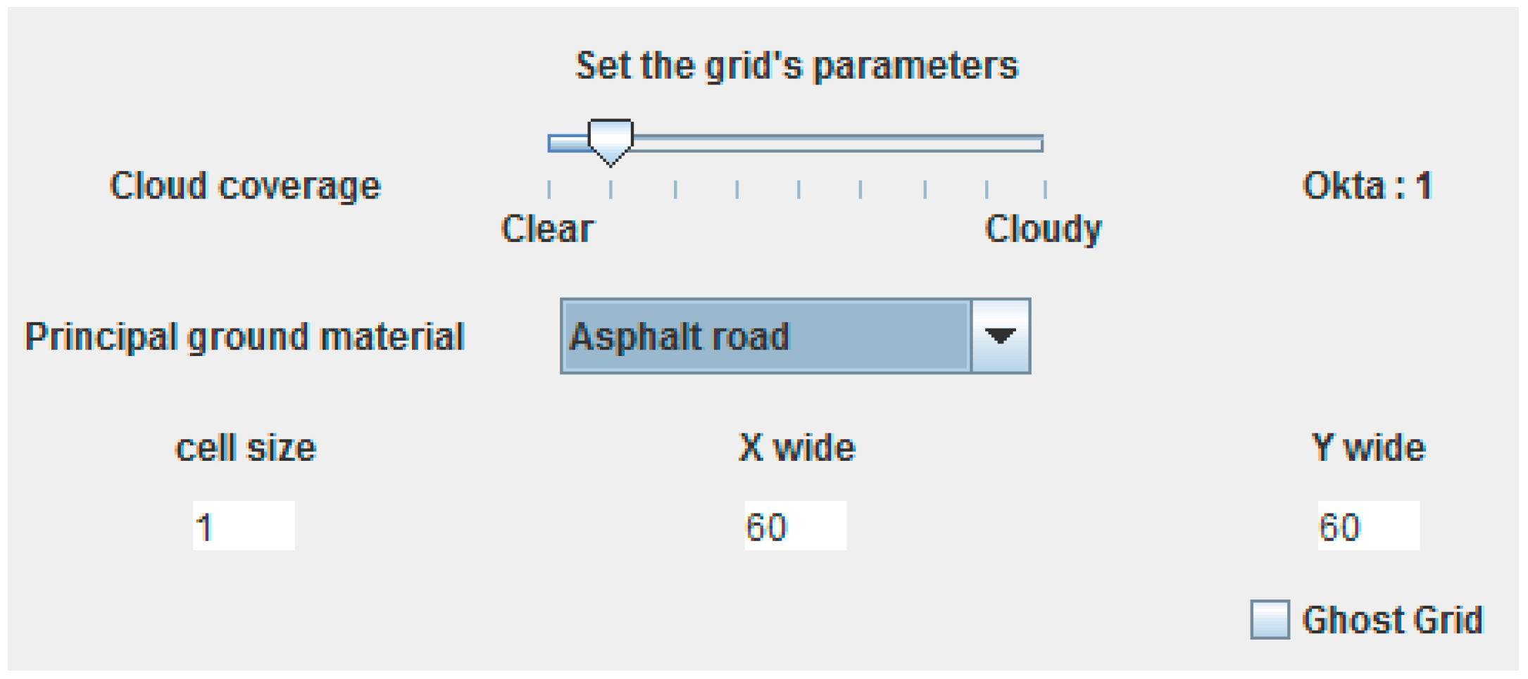
a dedicated control panel allows the setting of cloud coverage percentage and prevalent ground material, used for the estimation of the reflected component of the light ray;

(vi)

analytic grid size (Figure 6).

Figure 5. Panel to set geometric information of building and example for the procedure of using the aspect tool.

Figure 5. Panel to set geometric information of building and example for the procedure of using the aspect tool.

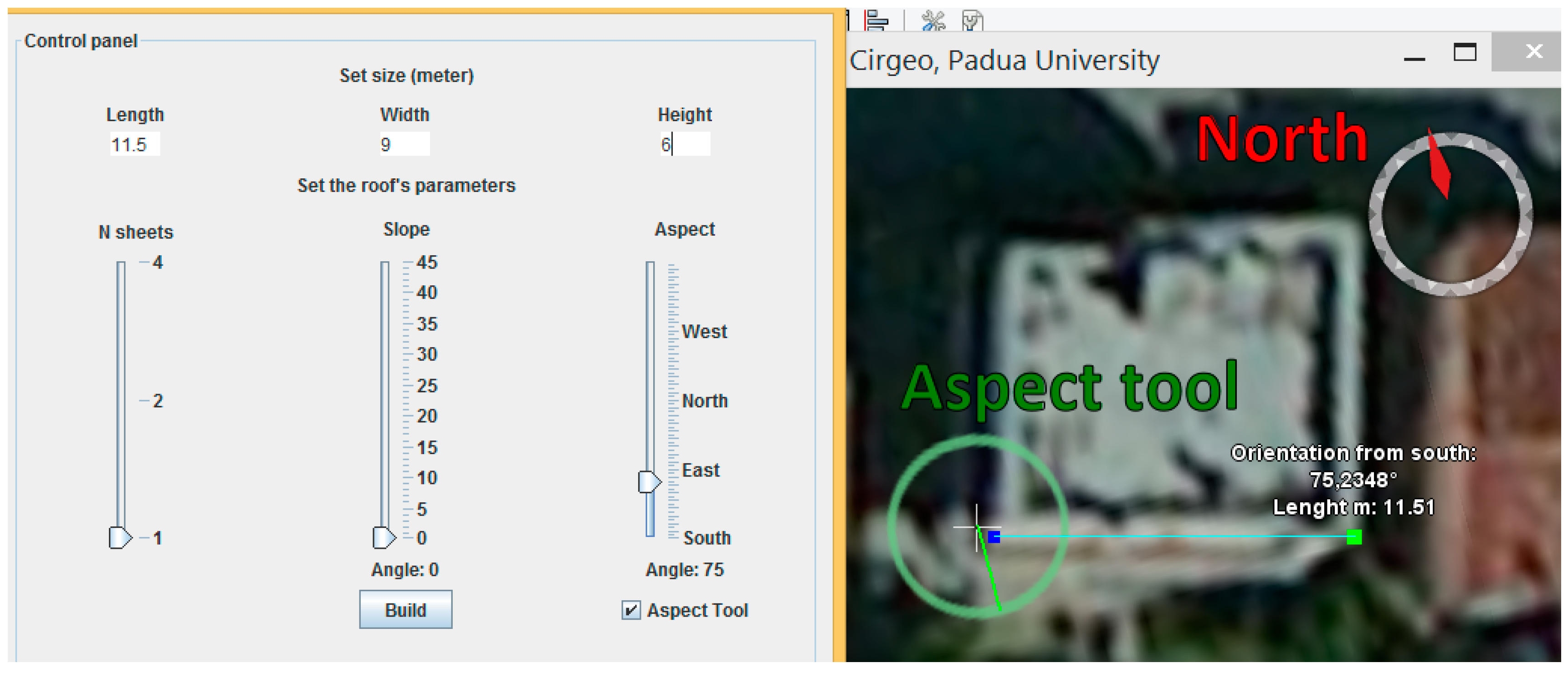
Figure 6. Tool to set the cloud coverage in 1 and principal material for reflection calculus.

Figure 6. Tool to set the cloud coverage in 1 and principal material for reflection calculus.

The size of grid is expressed in meters and the user can specify the number of cells in the X and Y directions. The final shape of the matrix can be square or rectangular. When the model is in execution, it computes the Sun’s position, the intersections of light ray with terrain and buildings, and the shadows on ground and buildings. The output products are two analytic surfaces of solar irradiance for the bare terrain (A) and for the non-terrain surfaces (i.e., roof tops) (B). The derived products are a merged surface (A and B), and a surface representing shadow areas. All surfaces are created using the information from the Sun’s position, obstructions’ geometry, aspect and slope of terrain morphology and atmospheric parameters. Shadow areas are colored differently due to buildings or elevation. Alternative visualizations of each layer can show the value of irradiance at the centroid of the grid cell. The simulation area chosen for a practical application is in the developer’s neighborhood in Padova City (Italy). Five buildings were created: one for each typology of roof and a fifth with a more complex geometry (Figure 7). Size and orientation can be measured using NASA WW base layers (e.g., orthophotos or cadaster map) as support and using a specific orientation tool. In the specific reported example the height is 6 m for buildings number 1, 2 and 5, 9 m for building number 4, and 3 m for building number 4. Roof angle is 30 degrees, and grid size is 60 × 60 cells, with each cell sampling 1 m at ground.

The model produces two analytics surfaces, one for ground and one for roofs. For each surface, a grid with values of irradiance is created. For each node, the model samples the NASA WW digital elevation model in order to calculate aspect and slope; it then merges results from the SPA with the atmosphere model and the 3D building model, calculating the values of irradiance in W/m². Values of 0 indicate shadow areas due to some obstacle in the Sun rays’ path (Figure 8).

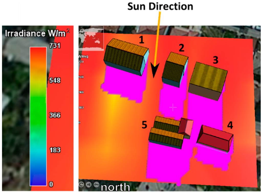
Figure 7. Simulation on 16 November 2014 at 12.31 pm with 1 m grid size in Padova. Violet areas indicate the shadows due to buildings.

Figure 7. Simulation on 16 November 2014 at 12.31 pm with 1 m grid size in Padova. Violet areas indicate the shadows due to buildings.

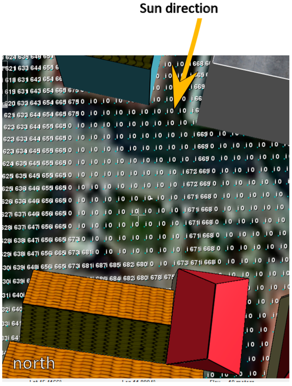
Figure 8. Values of irradiance W/m² in the ground grid nodes; 0 values indicate shadow areas.

Figure 8. Values of irradiance W/m² in the ground grid nodes; 0 values indicate shadow areas.

Roof analytic surface indicates which parts of the roof are in optimal positions to get the best irradiance, whereas shadow areas, due to building or elevation, are visualized as null values (empty parts) in the analytic surface (Figure 9).

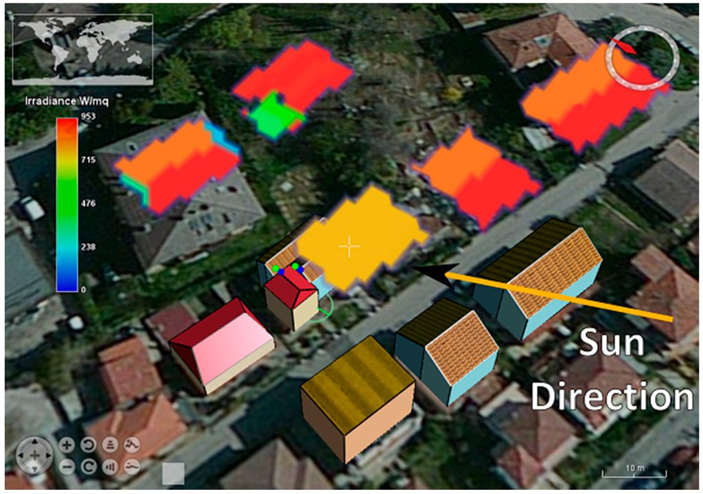
Figure 9. Roof analytic surface. Red areas indicate the sheets of roof with good irradiance: blue areas indicate the portion of roof with bad irradiance. Green dots and blue rays indicate shadow areas due to building obstruction.

Figure 9. Roof analytic surface. Red areas indicate the sheets of roof with good irradiance: blue areas indicate the portion of roof with bad irradiance. Green dots and blue rays indicate shadow areas due to building obstruction.

4. Conclusions

This model calculates two irradiance maps, bare ground and roof-tops, for a specific instant in time, which is set by the user. To be suitable for panel planning for photovoltaics, the next phase will be integration in time to produce an irradiation map based on a time interval (hour, day, month or year). The sky model used for this test is isotropic, which is considered accurate enough when considering a limited area (e.g., a single roof-top). Some other 3D tools use anisotropic models, and this improvement could be implemented easily, because the software is built with modular architecture and also offers functionalities to connect with a database where data on atmosphere are recorded. Future versions of this system will allow the integration of a user-defined terrain model, in order to allow a more accurate analysis of the study area. This capability is already available in NASA WW, and the focus of this future development will be to increase integration with the solar module to allow finer estimations of solar radiation. Future developments will also include the possibility of adding complete 3D models of cities uploading different 3D vector formats (e.g., City-GML, Collada), or deriving such information from 2D vector formats such as shapefiles with an attribute regarding the height of the buildings, therefore allowing extrusion of a simplified representation of the buildings. Extruded buildings are created as Java objects. A more precise model could represent the facades as Java objects and assign them attributes such as exposure and materials, or manage the presence of complexity, such as terraces and balconies. Each object thus created creates a more precise model but also introduces complexity into the system: a simple building with four facades becomes four objects, increasing computing time, energy, and memory requests. Vegetation is also another important factor that has to be studied in greater depth, as the complexity of vegetation types and their interaction with light in different seasons has to be modelled. Approaches have to be investigated to balance detail with required processing time, as more complexity adds more CPU cycles but does not always produce significant improvement over a more simplified model. One idea would be to classify tree species and provide canopy density classes that the user can choose from to accurately define the amount of solar radiation that can penetrate the canopy. This would allow enough level of detail to be significant when estimating the energy that gets obstructed by the canopy, which is complementary to the energy that enters the food-chain or energy balance in the case of ecological applications, [34]. To conclude, this investigation can lead to numerous applications which are of great interest to the community, not only from the point of view of a detailed model of the behavior of solar radiation and thus for planning renewable energy infrastructure [35], but also for ecological models and energy balance analysis, or to further improve other modules [36,37]. This first implementation can also be a starting point for further work by other researchers using NASA WW and interested at this scope.

References

- Hogan, P.; Gaskins, T. Geographic information processing: Standards-based open source visualization technology for environmental understanding. In GeoSpatial Visual Analytics; de Amicis, R., Stojanovic, R., Conti, G., Eds.; Springer: Dordrecht, The Netherlands, 2009; pp. 357–362. [Google Scholar]
- Bell, D.; Kuehnel, F.; Maxwell, C.; Kim, R.; Kasraie, K.; Gaskins, T.; Hogan, P.; Coughlan, J. NASA WW: Opensource GIS for mission operations. In Proceedings of the 2007 IEEE Aerospace Conference, Big Sky, MT, USA, 3–10 March 2007; Volumes 1–9, pp. 4317–4325.
- Rodríguez, E.; Morris, C.S.; Belz, J.E. A global assessment of the SRTM performance. Photogramm. Eng. Remote Sens. 2006, 7, 249–260. [Google Scholar] [CrossRef]
- Robertson, G.G.; Card, S.K.; Mackinlay, J.D. Information visualization using 3D interactive animation. Commun. ACM 1993, 36, 57–71. [Google Scholar] [CrossRef]
- Hildebrandt, D. A software reference architecture for service-oriented 3D geovisualization systems. ISPRS Int. J. Geo-Inf. 2014, 3, 1445–1490. [Google Scholar] [CrossRef]
- Green, M.A.; Emery, K.; Hishikawa, Y.; Warta, W.; Dunlop, E.D. Solar cell efficiency tables (version 42). Prog. Photovolt. Res. Appl. 2013, 21, 827–837. [Google Scholar] [CrossRef]
- Buriez, J.C.; Bonnel, B.; Fouquart, Y. Theoretical and experimental sensitivity study of the derivation of the solar irradiance at the earth’s surface from satellite data. Beitr. zur Phys. der Atmos. 1986, 59, 263–281. [Google Scholar]
- Gagliano, A.; Patania, F.; Nocera, F.; Capizzi, A.; Galesi, A. GIS-based decision support for solar photovoltaic planning in urban environment. In Smart Innovation, Systems and Technologies; Springer: Heildeberg, Germany, 2013; Volume 22, pp. 865–874. [Google Scholar]
- Rich, P.M.; Barnes, F.J.; Alamos, L.; Weiss, S.B. GIS-based solar radiation flux models. Am. Soc. Photogramm. Remote Sens. Tech. Pap. 1993, 3, 132–143. [Google Scholar]
- Dubayah, R.; Rich, P.M. Topographic solar radiation models for GIS. Int. J. Geogr. Inf. Syst. 1995, 9, 405–419. [Google Scholar] [CrossRef]
- Fu, P.; Rich, P.M. Design and implementation of the solar analyst: An ArcView extension for modeling solar radiation at landscape scales. In Proceedings of the Nineteenth Annual ESRI User Conference, San Diego, CA, USA, 26–30 July 1999; pp. 1–24.
- Neteler, M.; Mitasova, H. Open Source GIS: A GRASS GIS Approach; Springer US: New York, NY, USA, 2008; pp. 1–406. [Google Scholar]
- Hofierka, J.; Šúri, M. The solar radiation model for Open Source GIS: Implementation and applications. In Proceedings of the 2002 Open Source GIS-GRASS Users Conference, Trento, Italy, 11–13 September 2002.
- Hofierka, J. A new GIS-based solar radiation model and its application to photovoltaic assessments. Trans. GIS 2004, 8, 175–190. [Google Scholar] [CrossRef]
- Photovoltaic Geographical Information System (PVGIS). Available online: http://re.jrc.ec.europa.eu/pvgis/ (accessed on 17 December 2014).
- Šúri, M.; Cebecauer, T. SolarGIS: New Web-Based Service Offering Solar Radiation Data and PV Simulation Tools for Europe, North Africa and Middle East. Available online: http://geomodelsolar.eu/_docs/papers/2010/Suri-Cebecauer_SolarGIS_EUROSUN2010.pdf (accessed on 17 December 2014).
- Šúri, M.; Cebecauer, T.; Skoczek, A. SolarGIS: Solar data and online applications for PV planning and performance assessment. In Proceedings of the 26th European Photovoltaics Solar Energy Conference, Hamburg, Germany, 5–8 September 2011.
- Rylatt, M.; Gadsden, S.; Lomas, K. GIS-based decision support for solar energy planning in urban environments. Comput. Environ. Urban Syst. 2001, 25, 579–603. [Google Scholar] [CrossRef]
- Gadsden, S.; Rylatt, M.; Lomas, K.; Robinson, D. Predicting the urban solar fraction: A methodology for energy advisers and planners based on GIS. Energy Build. 2003, 35, 37–48. [Google Scholar] [CrossRef]
- PVsyst. Available online: http://files.pvsyst.com/help/index.html (accessed on 22 April 2015).
- PV*SOL. Available online: http://www.solardesign.co.uk/pv.php (accessed on 22 April 2015).
- Redweik, P.; Catita, C.; Brito, M.C. PV potential estimation using 3D local scale solar radiation model based on urban LIDAR data. In Proceedings of the 26th European Photovoltaic Solar Energy Conference, Hamburg, Germany, 5–9 September 2011; pp. 3–5.
- Erdélyi, R.; Wang, Y.; Guo, W.; Hanna, E.; Colantuono, G. Three-dimensional SOlar RAdiation Model (SORAM) and its application to 3-D urban planning. Sol. Energy 2014, 101, 63–73. [Google Scholar] [CrossRef]
- Ivanova, S.M. 3D analysis of the incident diffuse irradiance on the building’s surfaces in an urban environment. Int. J. Low-Carbon Technol. 2014. [Google Scholar] [CrossRef]
- Hofierka, J.; Zlocha, M. A new 3-D solar radiation model for 3-D city models. Trans. GIS 2012, 16, 681–690. [Google Scholar] [CrossRef]
- Tanaka, T.; Wang, M. Solution of radiative transfer in anisotropic plane-parallel atmosphere. J. Quant. Spectrosc. Radiat. Transf. 2008, 83, 555–577. [Google Scholar] [CrossRef]
- Reda, I.; Andreas, A. Solar position algorithm for solar radiation applications. Sol. Energy 2004, 76, 577–589. [Google Scholar] [CrossRef]
- Grena, R. Five new algorithms for the computation of Sun position from 2010 to 2110. Sol. Energy 2012, 86, 1323–1337. [Google Scholar] [CrossRef]
- Lee, C.-Y.; Chou, P.-C.; Chiang, C.-M.; Lin, C.-F. Sun tracking systems: A review. Sensors 2009, 9, 3875–3890. [Google Scholar] [CrossRef] [PubMed]
- Anderson, B. Solar Energy: Fundamentals in Building Design; McGraw-Hill: New York, NY, USA, 1977. [Google Scholar]
- Omini, G.; Savino, S. La Captazione dell’Energia Solare; CISM-Int Center Mech Sc: Udine, Italy, 2013; pp. 15–73. (In Italian) [Google Scholar]
- Kasten, F.; Czeplak, G. Solar and terrestrial radiation dependent on the amount and type of cloud. Sol. Energy 1980, 24, 177–189. [Google Scholar] [CrossRef]
- ENEA, Atlante Italiano Della Radiazione Solare. Available online: http://www.solaritaly.enea.it/CalcComune/Definizioni.php (accessed on 27 April 2015).
- Allen, R.G.; Trezza, R.; Tasumi, M. Analytical integrated functions for daily solar radiation on slopes. Agric. For. Meteorol. 2006, 139, 55–73. [Google Scholar] [CrossRef]
- Resch, B.; Sagl, G.; Törnros, T.; Bachmaier, A.; Eggers, J.-B.; Herkel, S.; Narmsara, S.; Gündra, H. GIS-based planning and modeling for renewable energy: Challenges and future research avenues. ISPRS Int. J. Geo-Inf. 2014, 3, 662–692. [Google Scholar] [CrossRef]
- Pirotti, F.; Guarnieri, A.; Vettore, A. Collaborative Web-GIS design: A case study for road risk analysis and monitoring. Trans. GIS 2011, 15, 213–226. [Google Scholar] [CrossRef]
- Piragnolo, M.; Pirotti, F.; Guarnieri, A.; Vettore, A.; Salogni, G. Geo-spatial support for assessment of anthropic impact on biodiversity. ISPRS Int. J. Geo-Inf. 2014, 3, 599–618. [Google Scholar] [CrossRef]
© 2015 by the authors; licensee MDPI, Basel, Switzerland. This article is an open access article distributed under the terms and conditions of the Creative Commons Attribution license (http://creativecommons.org/licenses/by/4.0/).