Abstract
The various levels of detail (LODs) of a 3D city model are often stored independently, without links between the representations of the same object, causing inconsistencies, as well as update and maintenance problems. One solution to this problem is to model the LOD as an extra geometric dimension perpendicular to the three spatial ones, resulting in a true 4D model in which a single 4D object (a polychoron) represents a 3D polyhedral object (e.g., a building) at all of its LODs and a multiple-LOD 3D city model is modeled as a 4D cell complex. While such an approach has been discussed before at a conceptual level, our objective in this paper is to describe how it can be realized by appropriately linking existing 3D models of the same object at different LODs. We first present our general methodology to construct such a 4D model, which consists of three steps: (1) finding corresponding 0D–3D cells; (2) creating 1D–4D cells connecting them; and (3) constructing the 4D model. Because of the complex relationships between the objects in different LODs, the creation of the connecting cells can become difficult. We therefore describe four different alternatives to do this, and we discuss the advantages and disadvantages of each in terms of their feasibility in practice and the properties that the resulting 4D model has. We show how the different linking schemes result in objects with different characteristics in several use cases. We also show how our linking method works in practice by implementing the linking of matching cells to construct a 4D model.
1. Introduction
Three-dimensional city models are characterized by their level of detail (LOD), a concept that describes their complexity and fineness, which is also related to their usability [1]. An increase in the detail of a model enables more applications, but means that its representations occupy larger sizes and their processing involves higher computational costs. Because of this, it is often desirable to have different LODs for the same 3D objects [2,3], similarly as in computer graphics [4]. For instance, the international standard for storing and representing 3D city models, CityGML [5], offers the possibility to jointly store data at multiple LODs [6].
However, the different representations of the same set of objects are usually stored separately and are either unconnected or connected only at the object level (e.g., through the use of IDs). This means that complex relationships between objects, such as collapses, aggregations and others that are not one-to-one, are difficult to store, which causes, among others, update and maintenance problems, as well as inconsistencies [7]. It also complicates the storage of semantic information about these relationships. Topographic maps, which are also available at multiple LODs, usually suffer from the same problems [8]. As further explained in Section 2, linking the representations on an object-to-object basis is unsatisfactory, because complex relationships, such as objects that are being displaced or multiple objects being merged into one, are only implicitly described.
As described in Section 3, an approach to solve the multiple independent representations problem is to model the LOD as an extra geometric dimension, which is independent and perpendicular to the three spatial ones. This makes it possible to store all correspondences between objects across discrete LODs by modeling them as if they were continuous and can be used for several applications, such as guaranteeing the consistency of a model across the LODs or the automatic update of datasets [9]. In the case of a model with three spatial dimensions, this implies constructing a true 4D geometric model in which the primitives are polychora embedded in 4D space, the 4D analogue of 2D polygons or 3D polyhedra, with every point having 4D coordinates of the form (), where l defines a point along the LOD axis. A true 4D model can then be stored using a variety of nD data structures [10], and a particular LOD can be obtained from the 4D model by ‘slicing’ it, i.e., computing its intersection with a certain surface or volume, at a predetermined point along the LOD dimension [11]. Note that this is opposed to the more common usage of the term ‘4D model’ in the GIS world, which refers to any system that handles temporal information in any manner, most commonly as a simple timestamp that is attached to every 2D/3D object.
We present in Section 4 four linking schemes that can be used to construct 4D models from a set of 3D objects, discussing the advantages and disadvantages of each method in terms of their feasibility in practice and of the properties that the 4D model would have. In Section 5, we present several use cases to demonstrate how the different schemes result in objects with different characteristics. The best scheme is therefore application dependent. For instance, one paradigm might be useful for visualization, while another one might be more suitable as the input of a noise modeling analysis. In Section 6, we show how our linking method works in practice by implementing the linking of matching cells to construct a 4D model. We conclude in Section 7 with a discussion and our ideas for future work.
2. Related Work
2.1. Level of Detail in 3D City Modeling
The general notion of the level of detail in 3D city modeling has been investigated by Biljecki et al. [1], who decompose the concept of LOD into multiple (mostly continuous) metrics, such as the geometric granularity, dimensionality, appearance and spatio-semantic coherence. The latter has been investigated in more detail by Stadler and Kolbe [12].
Meng and Forberg [13] and Fan and Meng [14] describe the scale space continuum of 3D buildings and define LOD as a milestone along the scale space. Döllner and Buchholz [15] also consider the LOD of a model as a conceptual dimension, allowing for the definition of continuous LODs. This is inline with our work, since we integrate the scale as an extra dimension, which requires parameterizing it.
Managing multiple LODs and switching between them is a topical problem in computer graphics [16], which has also influenced LOD management in 3D GIS [17]. Coarser LODs are usually generalized from finer LODs to improve visualization performances [18,19,20,21]
2.2. Identifying and Linking Corresponding Objects
In order to join multiple separate representations, stored as independent datasets, it is first necessary to find the correspondences between (equivalent) objects at different LODs. These independent objects can then be linked using various structures that have been previously described in the scientific literature, such as: hierarchical planar subdivisions [22], multi-scale partitions [23], nested maps [24] and topological generalized area partitioning trees [25].
The simplest linking schemes work within the context of an automatic generalization process [26], in which less detailed (i.e., generalized) versions of a model can be created algorithmically. In this case, the correspondences between objects at different LODs are known and can be linked during the generalization process [27].
Other methods attempt to find these correspondences using map matching methods, which can take into account the geometry [28], topology and semantics of and between the objects [29]. Devogele et al. [29] does this in three steps: (1) manually finding correspondences between semantic classes; (2) resolving conflicts; and (3) matching objects using geometry, topology and semantics. Zhang et al. [8] matches features by computing a compatibility coefficient, derived from the similarity in their geometry and that of their neighbors. Biljecki et al. [7] detect identical geometries across multiple LODs of the same object in a CityGML file and reuse them to obtain a smaller file size.
2.3. LOD as a Dimension
Döllner and Buchholz [15] discusses the concept of a continuous LOD that can be used to model discrete LODs. Although this is not directly related to the LOD as a dimension, it enables the LOD to be modeled in this manner by parameterizing the LOD, such that it can be placed in an axis.
Van Oosterom and Meijers [30] discuss the integration of 2D maps at different LODs in one model that is conceptually 3D (2D + LOD), the space-scale cube (SSC). The polygonal areas in a map are stored as a hierarchy of 2D planar partitions at different LODs, which are linked together. However, as this approach does not use actual 3D objects, only the operations that are encoded into the logic of its algorithms can be supported (i.e., line generalization and merging of areas).
They also discuss a conceptual generalization of the SSC to 4D, i.e., where volumes are used as input and the level of detail becomes the fourth dimension. However, their description is only theoretical: there is no attempt to construct or store a 4D model. Furthermore, the only case considered is two adjacent rectangular prisms being aggregated and then simplified to a higher scale. Constructing the 4D model for such a case is the simplest of the four cases we consider in Section 4, because both input objects have the same topology, and finding a correspondence between primitives is thus straightforward.
2.4. Storing a 4D Model
There are a few nD data structures that can be used in order to store a 4D model in a computer; Arroyo Ohori et al. [10] give a complete overview. The simplest ones involve extensions of the 2D/3D raster [31,32] and hierarchical subdivision [33,34] representations common in GIS. These can use similar structures and algorithms as their 2D/3D counterparts and are therefore easy to implement, but are only capable of achieving rough approximations of the boundaries of the objects and grow in size exponentially as the dimension increases. Vector data structures with limited topological information, such as simple features [35] or incidence graphs [36,37,38], possibly combined with the computation of topology on the fly [39], also become intractable in higher dimensions. Implicit models, such as constructive solid geometry and Boolean set operations on half-spaces, are not sufficient by themselves and generally have to be converted into another, more explicit, model in order for them to be analyzed and visualized [40].
Because of these shortcomings, the most promising option is to use topological vector nD data structures. Some of these structures involve the subdivision of all objects into geometric simplices (i.e., the generalization of 2D triangles and 3D tetrahedra to arbitrary dimensions) forming a simplicial complex. There are several such structures [41], which tend to be conceptually simple and easy to implement. However, performing the subdivision of each object into simplices requires using a constrained or conforming triangulation [42,43], which is very hard to realize in practice in more than three dimensions (since there is no known available software).
Ordered topological models, which are able to represent more general cell complexes using the internal structure of a simplicial complex, therefore, have clear advantages. Generalized maps (g-maps) [44] and the cell-tuple structure [45] are capable of storing a large class of cell complexes, including orientable and unorientable manifold objects of arbitrary dimension, including objects with boundaries by Poudret et al. [46]. They have been implemented in libraries and software, including Moka and Gocad. Combinatorial maps [44] require defining an orientation for the objects, but use half the storage space of generalized maps. They have also been implemented in mature libraries, such as CGAL and CGOGN [47].
2.5. Construction Algorithms for a 4D Model
We have previously developed two low-level construction algorithms for nD objects. These can be used as a base to create 4D models in following manner: (1) when the 3D objects remain relatively unchanged along the LOD dimension, the 4D model can be extruded from 3D to 4D, creating simple prismatic objects, which are possibly further processed; or (2) when arbitrarily shaped 4D models are needed, the individual faces and volumes on the boundary of the 4D model are incrementally constructed and linked.
The first approach uses a dimension-independent extrusion operator [48,49]. It ‘lifts’ a n-dimensional model into -dimensional space by assigning each n-dimensional object a range along which it exists, generating a set of prismatic polytopes, analogous to prisms in 3D. Intuitively, this new cell complex consists of ‘base’ and ‘top’ faces constructed from the original cell complex, with and respectively added as n-th coordinates in their zero-attributes. These ‘base’ and ‘top’ are joined by a set of additional prismatic faces linking corresponding -cells (ridges) of the base and top cells. This method is poorly suited for our case, since the two LODs have to have the same topology, which is rare in practice (we show in Section 4 that in almost all cases, they differ significantly).
The second approach, which is more generic and more suitable to our case, allows us to use the arbitrary cell complexes that have been generated using the linking rules presented in this paper. This entails that all of the bounding volumes linking two models have to be generated first, starting from defining all of the necessary 4D points of the form , where are the three spatial dimensions and l is a point on the LOD axis. These are then linked in increasing dimension to form faces, volumes and the four-cell for each 4D object. The schemes for generating these are described in Section 4.2, and these can be appropriately linked together using the incremental construction operator [50], which takes a set of -cells forming a closed i-cell and joins them along their common -cells (ridges) to create the aforementioned i-cell by generating all of the topological relationships between them.
2.6. Slicing to Extract a 3D Model at a Certain LOD
In order to obtain a 3D model from an integrated 4D model at a certain LOD, it is possible to reduce the dimension of a spatial object by slicing [11]. In this operation, a higher-dimensional set of objects is geometrically intersected with another lower-dimensional object, often unbounded along some dimensions and orthogonal to the axes of the others. The end result can then be given in terms of the lower dimensional space induced by this object, which is equivalent to an orthographic projection of the intersection to a coordinate system describing the vector space where it lies.
In order to extract a 3D model at a certain LOD l from a 4D model, the object used is an unbounded 3D volume embedded in 4D. This is similar to how an unbounded plane can be embedded in 3D to generate a cross-section of an object. The unbounded 3D volume is therefore a region of 3D space that is similar to and orthogonal to the LOD axis l, covering the range along the three spatial dimensions and having a single value along the LOD axis l. Note that although in the continuation of this paper, we consider only orthogonal slicing along the LOD axis (producing a 3D model of a fixed LOD), mixed-LOD models obtained from non-orthogonal slices planes are possible: Van Oosterom and Meijers [30] demonstrate one case in 3D (which has not been generalized to 4D).
3. Methodology to Model LOD as an Extra Geometric Dimension in a True 4D Model
Incorporating non-spatial characteristics as additional dimensions in the geometric sense results in a fabric of higher-dimensional space where objects can be embedded. As an extension of the standard spatial data modeling concepts, this space can be modeled as the d-dimensional Euclidean space . In this manner, each dimension is defined by an independent (perpendicular) axis, and a point in this space is defined by an d-tuple of coordinates.
This higher-dimensional space is then populated by a set of objects of dimension from zero (i.e., points) up to d (i.e., d-polytopes). These are non-overlapping and, thus, together with the empty space surrounding them, induce a partition of the space, analogously to a set of polygons forming a planar partition in 2D. As is usual in GIS, we will assume that these objects have linear (i.e., flat) geometries, which significantly simplifies their representation and most operations.
In the specific case of a 4D (3D space + LOD) model, this means that we have an additional LOD axis l, and a point in 4D space is defined by a tuple of coordinates . It is worth noting that the LOD axis should be properly parameterized, defining quantifiable values for every fixed LOD in a model or, alternatively, a function that does so.
The 4D space is filled with a set of non-overlapping polychora, in which a 3D object (e.g., a building) at all of its different LODs is represented as a single 4D object. This 4D object is bounded by a set of volumes, two of them being the object at its lowest and highest LOD and several lateral ones formed by filling the space between corresponding faces across LODs. When sliced, these respectively correspond to the volumes and bounding faces of an extracted 3D model.
Observe that a true 4D model permits us not only to link the different representations of an object together, but it goes further, since it enables us to model and store explicitly more complex relationships between the objects. An example is when multiple objects are merged into one; this case is cumbersome to handle with IDs (which ID should the new object get?); however, if the topological relationships between the objects are explicitly stored, it suffices to analyze these to detect such a case. If the multiple objects would be simultaneously changing along multiple parameters, such as changing shape (e.g., because of a simplification process) and moving over time, then another dimension (time) could be added to the model, as well, yielding a 5D model [9] that can be represented as a set of 5D objects modeled as a 5D cell complex. Such a model could be represented as a 5D cell complex with an analogous definition as the 4D cell complex presented here. Note that although this is a straightforward change in terms of the model and its storage, 5D operations to create and manipulate such objects would have to be developed in order to make such a model useful.
We represent mathematically the aforementioned 4D model with a 4D cell complex, a subdivision of space into cells, such that for all , an i-dimensional cell (i-cell) is a topological object homeomorphic to an i-ball (e.g., point, segment, disk, ball, etc.). For all , every i-cell in the complex has a number of -cells (faces) as its boundary, which are also part of the complex. The common boundaries of two i-cells is given by their intersection, returning a set of -cells, which are also part of the complex. Every zero-cell (i.e., a vertex) is attached to a tuple of coordinates representing a point in 4D space. This 4D cell complex can then be stored in any of the data structures presented in Section 2.4.
4. Constructing a 4D Model from a 3D City Model and Its LODs
The buildings in a 3D city model are often modeled in multiple LODs. For instance, in the CityGML standard [5], five discrete LODs can be stored (from the 2D footprint of the building up to a representation where the windows, doors and walls and even indoor objects are all modeled in detail). These different representations are in most cases not derived from the most detailed LOD (e.g., with generalization methods), but are collected with different techniques, often for different purposes, and thus, the resulting representations do not necessarily have easy-to-identify correspondences. The same object can be slightly displaced at different LODs; an object can be an aggregate of other objects (think of a terraced house: either each house is represented or one volume for the whole row) or can be modeled in an entirely different way.
The construction of a 4D model from existing LODs of a 3D city model consists of three steps:
- Identifying corresponding 0D–3D cells;
- Linking them by creating 1D–4D cells connecting them;
- Using an incremental construction algorithm [50] to build a 4D cell complex using all 0D–4D cells.
We first present in this section various methods to identify corresponding cells in different LODs of a 3D object (Section 4.1), and then, we present four linking schemes to construct a 4D model (Section 4.2). As we demonstrate in Section 5 on use cases, the 4D cells created by the linking schemes are used to construct 4D cell complexes with different properties and shapes, each of which has its own requirements.
4.1. Step 1: Identifying Corresponding Cells in 3D Models
Constructing a 4D model from a sequence of 3D models largely depends on the identification of the corresponding 0-, 1-, 2- and 3-cells between these 3D models. The aim of this identification is to create a mapping between the 3D models that preserves the topological relationships between the elements in the models, so as to create a valid 4D model.
Considering 3D models at different LODs, this identification will often result in matching cells of different dimensions, commonly with some cells in the 3D model at the highest LOD being matched to cells of lower dimension in the 3D model at the lowest LOD. Furthermore, these correspondences will often not result in a one-to-one mapping: groups of adjoining cells in one model, most often in the one at the highest LOD, will commonly be matched to a single cell in the other model.
The identification of matching cells should be done using a combination of the following, arguably in order of preference:
Attributes: Use the semantic information stored in the cells, when it is available. For instance, matching two cells that are known to be equivalent through the use of IDs or, if knowledge is kept during the generalization process, matching a cell with one that is known to be a simplified version of it.
Topology: When there is a one-to-one mapping (a bijection) between two cells that preserves all of their topological relationships, this mapping is known as an isomorphism and the cells are said to be isomorphic. Therefore, an isomorphism between two cells already gives a matching between them, although it might be important to check that the isomorphism is compatible with the matching of the other cells in the model and with geometric constraints. Relevantly, Gosselin et al. [51] describe how to compute isomorphism in a generalized map of any dimension. Another more complex possibility is using subgraph isomorphism on unmatched portions of a generalized map [52], even if this problem is known to be NP-complete.
Another way to use topology is to use the topological relationships between cells in order to infer matchings for the remaining cells [27]. This is explained more concretely in the example of Figure 3.
Geometry: Use geometric computations, such as those based on computing similarity metrics, simply matching unmatched cells in one model to their nearest neighbor in another model or attempting to minimize the Earth mover's distance (EMD) [53] between them. It is, however, important to compute these matches using constraints that generally preserve the relative positions and topological relationships between the cells. For instance, a greedy algorithm could match cells iteratively, cascading these matches to adjacent cells (in all models) or rejecting matches that would violate a geometric or topological constraint.
A final possibility to assist when matching cells is to allow splitting an i-cell into multiple i-cells by adding cells of lower dimensions in a manner that does not alter the geometry of the cell. For instance, a face can be split into multiple faces by adding a vertex in its interior and creating edges that link it to some of the vertices of the face. This can make two cell complexes isomorphic and directly allow for a one-to-one mapping between two cell complexes.
4.2. Step 2: Linking Corresponding Cells
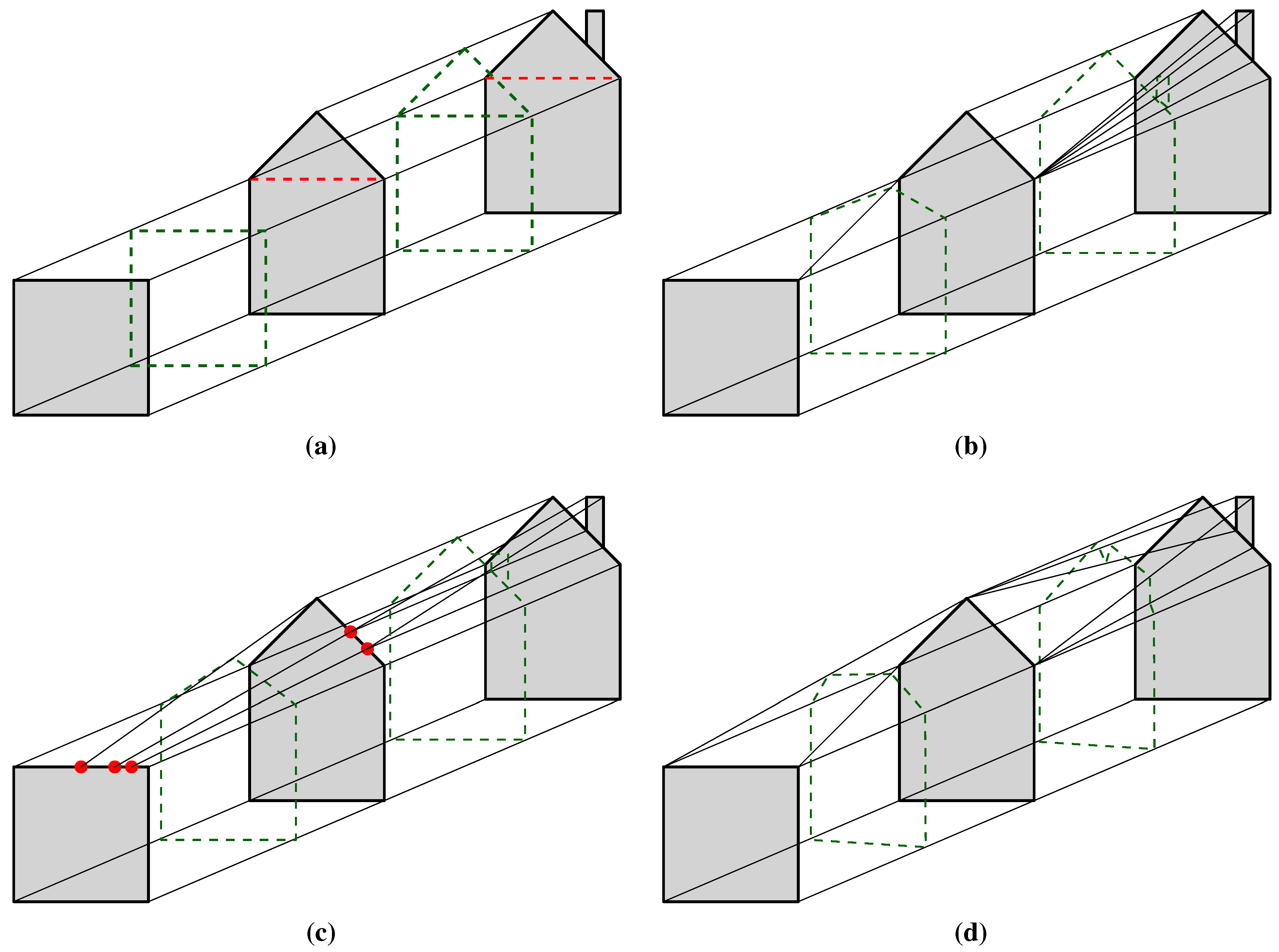
Based on the matches that were found between cells, which mathematically define a map between the 3D cell complexes of the 3D models, we can subsequently link them to construct a 4D cell complex. For this, it might be necessary to create or modify 0D–3D cells in the input cell complexes, as well as to create new 1D–4D cells that lie between the cell complexes. The resulting 4D cell complex is then embedded in 4D space by assigning new 4D coordinates for every point. We propose four different basic linking schemes, which are shown in Figure 1.
4.2.1. Method 1: Simple Linking of Corresponding Cells
Links are constructed between the corresponding cells of an object at two different LODs, and if a cell has no corresponding cell, then it is ignored. While this allows us to easily construct a 4D cell complex in the cases where all cells in the lower LOD model have a corresponding cell in the higher LOD model, when this is not the case, the result will consist of an incomplete 4D cell complex.
To ensure a complete one, cells often need to be split (e.g., those separated by the red dotted line in Figure 1a), which can be performed using geometric intersections. While this is possible in 3D and tools are readily available (see, for instance, Granados et al. [54], Hachenberger [55]), it should be noticed that the generalization of this scheme to higher dimensions (i.e., 5D +) is not easy in practice, since no robust intersection tools in more than 3D are available. Observe that if a 4D cell complex generated using this method is sliced at an intermediate LOD, the result is exactly that of the lower LOD.
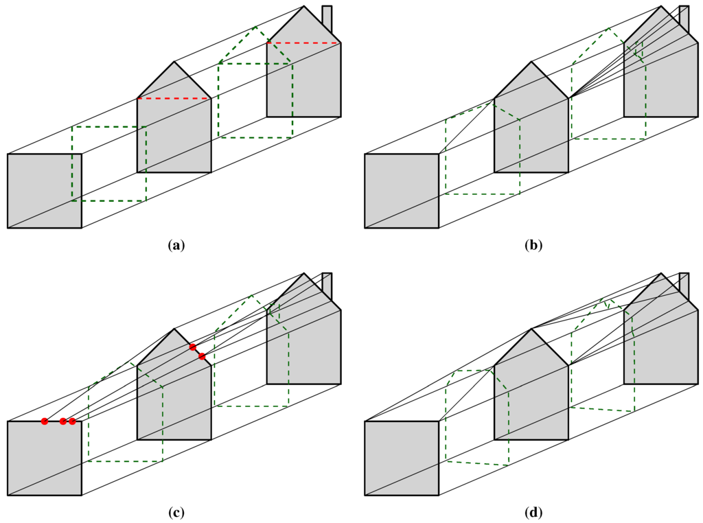
Figure 1.
The four linking schemes for three levels of detail (LODs) of a house, here depicted in 2D: (a) simple linking. (b) unmatched are collapsed. (c) modification of topology and (d) matching all to existing. The objects that would be obtained by slicing between the LODs can be seen in dashed green contours; the red dashed lines reflect the cells that need to be added and split in order to ensure a valid 3D (2D + LOD) cell complex.
4.2.2. Method 2: Unmatched Cells Are Collapsed into Existing Ones
No modifications are made to the 3D models, which is in practice a significant advantage, since no complex geometric operations need to be performed and the size of the cell complex will be smaller than that of the one where cells are modified. Instead of geometric operations, unmatched cells in the higher LOD model are linked to nearby matched cells of a possibly lower dimension in the lower LOD model while preserving certain geometric and topological constraints (e.g., preserving adjacency and incidence between cells). This implies that some cells will be collapsed (e.g., an edge can be mapped to a vertex), and the cells must be linked with care to ensure that a valid 4D cell complex is created (e.g., no two cells should intersect).
For instance, assume that the left eave of the roof of the house in the middle LOD model in Figure 1b has been (arbitrarily) matched to the roof of the low LOD model, with the right eave remaining unmatched, as no unmatched cells remain in the low LOD model. In this case, using the knowledge that the roof and right wall are adjacent in the low LOD model, but their corresponding cells (respectively the left eave and right wall) are separated by the right eave in the middle LOD model, the right eave can be collapsed to the common vertex lying between the two (upper right). Using such a mapping, the topological relationships between the cells will be preserved, with the exception of those involving the collapsed cells and those incident or adjacent to them.
Notice that when the mapping has faults and the resulting 4D cell complex thus has geometric problems (e.g., intersecting cells), the slicing operation might not have any geometric meaning, but the main advantage of the integration (consistency) will nevertheless still be guaranteed for all other cells. Ensuring that cells preserve their topological relationships and form a partitioning of space in 4D is challenging and is part of our future work. Finally, observe that even if a combinatorially- and geometrically-valid 4D cell complex is constructed, the 3D object obtained by slicing might not be consistent with reality; notice how the chimney in Figure 1b becomes increasingly smaller and closer to the right eave of the roof, because of the way the cells have been linked.
4.2.3. Method 3: Modifying the Topology
To ensure that there is a mapping between all of the cells, we can split or merge cells so that the topology (combinatorial structure) of the objects is identical. For instance, operations like removal and contraction [56] can be used to simplify the more complex object(s) to make them match the simpler one(s) using an iterative process. On the other direction, it is possible to first identify for every cell in the lower LOD model one or more corresponding cells in the higher LOD model, then split cells in the lower LOD model, so that their topology is the same as in the higher LOD model as the one to which it must be linked.
In Figure 1c, for the lowest LOD, this implies first finding multiple matches for the roof cells of the lower LOD models, which then need to be split into multiple cells by the insertion of new vertices. For instance, these can be located at the closest location that lies on the matched lower LOD cell for every higher LOD cell. As this example shows, all of the representations of an object where this approach is used will end up having the same topology. This results in increased storage space and the possibility of degenerate cells e.g., multiple vertices at one location. The geometric operations necessary to split cells can be rather intricate, as well. Observe that slicing however results in a different representation of the object one where it smoothly morphs into the one at lower LOD (e.g., the tip of the roof is slowly lowered as the LOD decreases).
4.2.4. Method 4: Matching All Cells to Existing Ones
As is the case with Method 2, this method does not require modifying the topology of the objects. The main difference with it is that cells in the higher LOD model are not necessarily collapsed to a lower dimensional cell in the lower LOD model, but are instead matched to one or more cells of any dimension, while also preserving certain geometric and topological constraints. In Figure 1d, observe that the tip of the roof of the middle LOD model (a point) is matched to the roof of the lowest LOD (an edge, since we have a 2D representation) and that the two edges representing the middle-LOD roof are matched to the two corners of the lower-LOD roof (points). Slicing thus creates a truncated roof having three edges. This can be achieved by matching all cells that have a clear correspondence first, then attempting to match groups of unmatched cells while preserving the topological relationships between cells.
For instance, in Figure 1d, it is possible to first match the base and walls of the houses in the lower and middle LOD models, then match the remaining vertex and left/right edges in the middle LOD model respectively to the roof edge and left/right vertices. Observe that in this process, the tip of the roof of the middle LOD model (a point) is matched to the roof of the lowest LOD (an edge) and that the two eaves of the roof (edges) are matched to the two corners of the roof (points) in the lowest LOD. Slicing the resulting 4D cell complex creates a truncated roof having three edges. The matches for the chimney to other elements in Figure 1d are achieved by matching the chimney top to the right eave and the remaining vertices and edges to its left and right sides respectively to the roof tip and right eave/wall vertices. The result is that while the chimney looses resemblance to reality, it slowly converges to the roof in the middle LOD model.
5. Use Cases
We present in this section practical examples that describe the matching and the linking of cells for a few simple 3D models representing the same object(s) at different LODs.
5.1. Using Method 1: Simple Linking
Figure 2 shows an example where two LODs for a building are linked in such a way that only matched cells are involved.

Figure 2.
Two LODs of a house simply linked and the intermediate LOD obtained.
Figure 2.
Two LODs of a house simply linked and the intermediate LOD obtained.
First, observe that since the two objects are not isomorphic, some cells are not matched (the ones representing the roof of the higher-LOD model). Observe also that the roof of the lower-LOD model has no match in the higher-LOD model. Thus, to construct a 4D cell complex, the flat roof geometry has to be added to the higher-LOD model. Then, the corresponding cells can be linked. Although it is possible to generate this 4D model by generating the -cells that connect a pair of corresponding i-cells and linking all of them together, it is easiest to extrude one cell complex along the range between the two LODs.
This already generates the proper combinatorial structure of the 4D model, and the final cell complex can be obtained by then moving the vertices of the face representing the model at the other LOD so as to match the geometry of the other model at its LOD. Moreover, since we are assuming a linear cell complex and thus only the vertices are storing the geometry of the model, it is only necessary to move the vertices at the lowest LOD without a corresponding vertex at the highest LOD.
5.2. Using Method 2: Collapsing
Figure 3 shows an example with a 3D model at two LODs with differing geometry and topology.
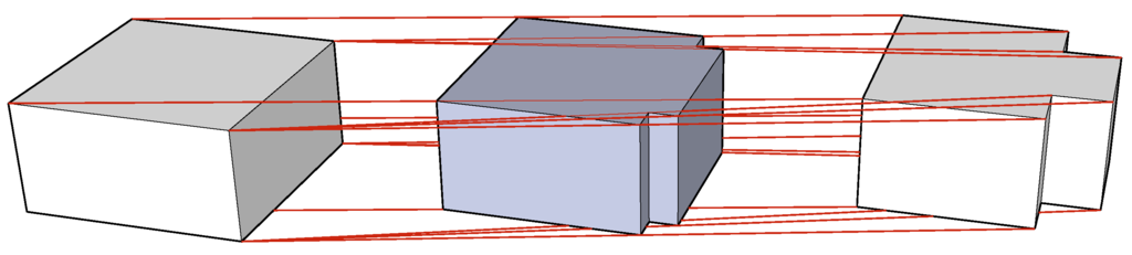
Figure 3.
Two LODs of a house with differing geometry and topology are integrated into a 4D model by collapsing cells in the model at the highest LOD.
Figure 3.
Two LODs of a house with differing geometry and topology are integrated into a 4D model by collapsing cells in the model at the highest LOD.

The 4D model has been obtained by first matching the two cells with known correspondences (the left, right, front and back large faces) and inferring that the other faces in the model at the highest LOD (right) should be collapsed based on their adjacency relationships with the matched faces. For example, since the front and right faces are adjacent in the lowest LOD, but not in the highest LOD, the two faces between them should be collapsed into their common boundary (i.e., their intersection: the edge between them). Combinatorially, this involves a search for a path between the front and right faces in the graph of the model at the highest LOD, such a search being limited to the nodes representing the aforementioned faces and those representing faces that are not present in the model at the lowest LOD. This example also shows that the topological relationships between the cells are nevertheless preserved with the exception of those that involved collapsed cells. The new topological relationships do however connect cells around the former collapsed cells. Note that the 3D model resulting from slicing the 4D model created in this way at an intermediate LOD (middle) will be isomorphic to the model at the highest LOD.
5.3. Using Method 3: Modifying the Topology
Figure 4 shows an example of two 3D models being aggregated.
In order to create a 4D model from this situation, the topology of the simpler of the two models is modified, splitting the single volume into equal two adjacent ones, effectively resulting in a cell complex that also has four more vertices, four more edges and four of its faces split into two. Note that the two models are however not isomorphic, since the common face of the two houses in the lowest LOD becomes two disconnected faces in the model at the highest LOD, but that if we disregard this topological relationship, the two models can be correctly matched independently.
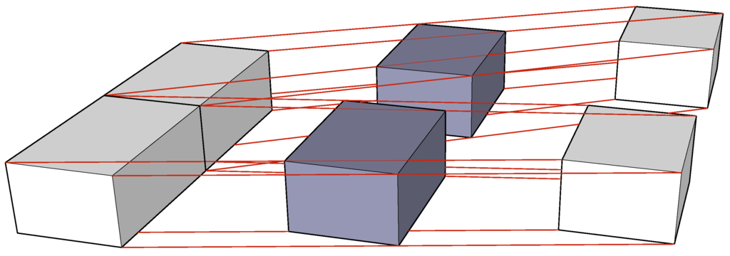
Figure 4.
Two LODs of two houses being aggregated are integrated into a 4D model by modifying the topology of the model at the lowest LOD so as to match the topology of the model at the highest LOD.
Figure 4.
Two LODs of two houses being aggregated are integrated into a 4D model by modifying the topology of the model at the lowest LOD so as to match the topology of the model at the highest LOD.

5.4. Combination of Methods 2 and 3
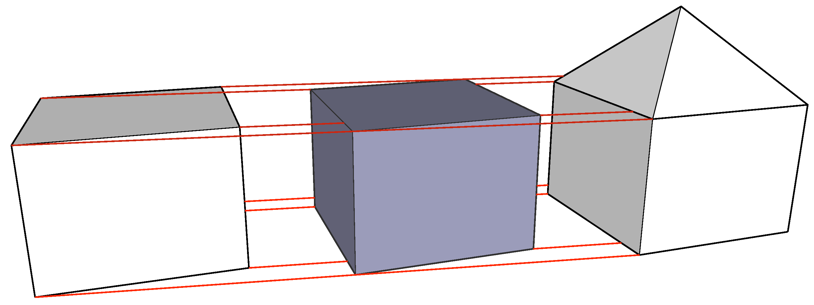
Figure 5 shows a more complex example with three LODs, which are linked using a combination of schemes: collapsing and modifying the topology of one of the models.

Figure 5.
Three LODs of a 3D model of a house are integrated into a 4D model by modifying the topology of the model at the lowest LOD and collapsing a part of the model in the highest LOD.
Figure 5.
Three LODs of a 3D model of a house are integrated into a 4D model by modifying the topology of the model at the lowest LOD and collapsing a part of the model in the highest LOD.
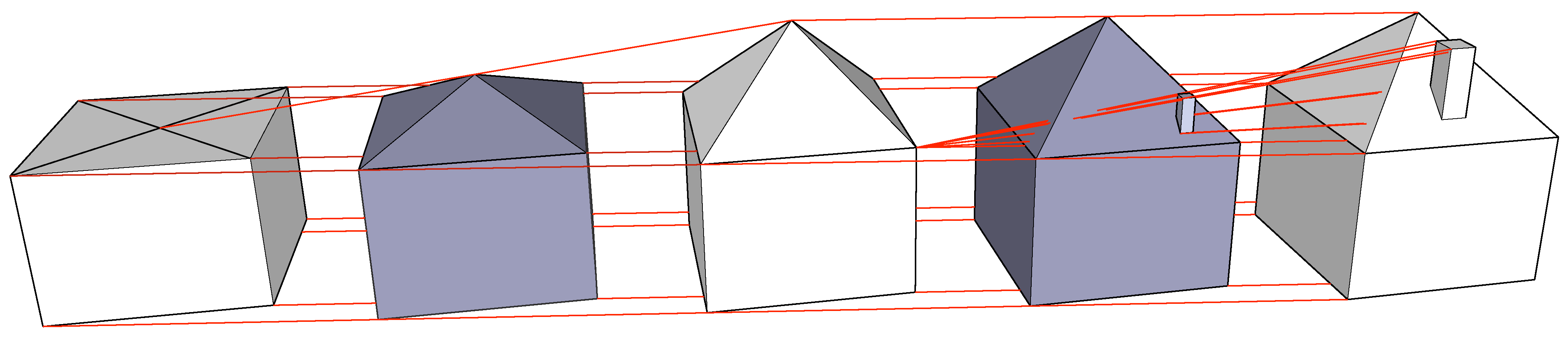
Most of the cells in the highest LOD can be directly matched to cells in the middle LOD, with the exception of those that are part of the chimney. As these comprise a small object, these are simply collapsed into a single point in the middle LOD. Matching the roof cells in the lowest and middle LODs is, however, more complex, since collapsing it into a point would ignore its adjacency with the body of the house and, therefore, not preserve its topology. The best solution is therefore to modify the topology of the lowest LOD in order to split the top face of the cubic house (which we know is a roof based on its attributes) into four faces, making the model isomorphic to the middle LOD.
5.5. Using Method 4: Matching to Existing Cells
Figure 6 shows two of the LODs of the previous example, but matches the cells of the roof of the house to existing cells rather than modifying their topology.
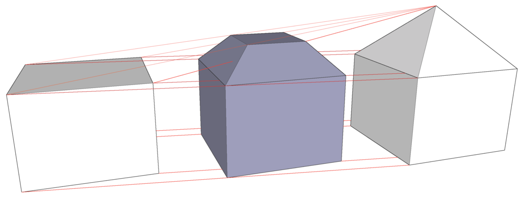
Figure 6.
Two LODs of a 3D model of a house (left and right) are linked despite not being isomorphic, with an intermediate LOD that shows the result of slicing the construction at an intermediate LOD (center).
Figure 6.
Two LODs of a 3D model of a house (left and right) are linked despite not being isomorphic, with an intermediate LOD that shows the result of slicing the construction at an intermediate LOD (center).

After attempting to match corresponding cells, the top face in the lowest LOD and the top four faces in the highest LOD remain unmatched. If we collapse each top face in the highest LOD to the closest top edge in the lowest LOD (i.e., the edge that forms the bottom of the triangular face in the highest LOD) and the top vertex in the highest LOD (which lies between the faces) is linked to the top face in the lowest LOD, a four-sided pyramid is generated. Slices from it are shown as four trapezoidal faces in the sliced intermediate LOD. Then, if we collapse, the top face in the lowest LOD to the top vertex of the highest LOD, another four-sided pyramid is generated. A slice from this one is shown as a square face at the top of the sliced intermediate LOD.
This particular mapping, which correctly preserves all topological relationships between the cells, is interesting, since it shows that cells are not necessarily only collapsed from higher LODs to lower LODs. It is worth noting that the result of this mapping is a set of cells that bound the model along the LOD dimension, so that an i-cell and a j-cell that are matched result in a k-cell lying between them, where . Concretely, if, for instance, a zero-cell (the tip of the roof) is matched to the flat roof (two-cell), then the resulting links will create a tetrahedron (a three-cell). Note also that although the rules needed to generate such a mapping might be more complex, the cell complex generated is identical in size as the equivalent model according to the scheme in Figure 1b.
6. A Concrete Example: Implementing Cell Matching to Construct a 4D Model
In order to show how our linking methods work in practice, we have implemented the model shown in Figure 6 using CGAL Linear Cell Complexes and the incremental constructor operator described in Arroyo Ohori et al. [50]. This model was chosen as it uses most of the linking methods discussed in the Section 4.2: the body of the house in both LODs is directly linked (Method 1); the top face of the house in the lower LOD is collapsed into the tip of the roof in the higher LOD (Method 2); and the roof vertices/edges in the lower LOD are connected to existing roof edges/vertices in the higher LOD (Method 4).
First of all, the 17 vertices of the two 3D models are created as 4D points of the form . Afterwards, these are first used to define the 35 faces of the model; the faces are used to define the 12 volumes and the volumes to define the single four-cell. Notice that these include faces and volumes within each of the two volumes of the input 3D models, but also include some faces and volumes that lie between the two, i.e., having vertices and faces in both input 3D models. Excerpts of the code to generate the 4D cell complex are shown in Figure 7.
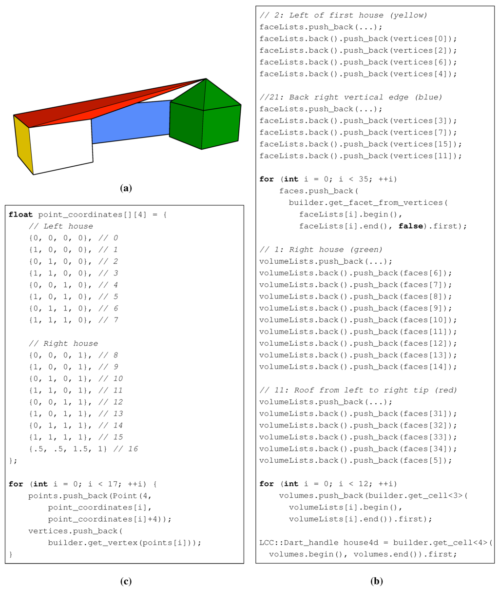
Figure 7.
Code excerpts that show how (a) a 4D model of the house shown in Figure 6 is constructed. (b) faces are created as cycles of vertices, volumes as sets of faces and four-cells as sets of three-cells. (c) vertices are created based on 4D points. The colors referred to in (b) correspond to the highlighted faces and volumes in (a).

The resulting 4D model was then validated by checking the properties of a valid combinatorial map (cf. Lienhardt [44]). In short, we tested whether the darts (combinatorial simplices) in the map formed correct involutions or permutations and whether any darts remained free after the operations. We also validated individual parts of the model (the triangular or square faces and the parallelepiped- or pyramid-shaped volumes) by verifying that they were isomorphic to similar objects that were known to be valid [51].
7. Discussion and Future Work
While integrating different LODs of the same 3D object in a 4D model is technically more complex than maintaining them separately, we have shown that it is possible to create such a 4D model by identifying matching elements in different LODs, linking them to obtain 4D primitives and, finally, constructing and storing a 4D cell complex with algorithms and data structures that are readily available. We believe the advantages of this integration to be many.
First, it provides a fundamental solution to the maintenance of these models since any update could be propagated to other LODs; consistency of the model at all LOD can thus be ensured, e.g., using the validity checks in Gröger and Plümer [57]. Such a 4D model thus supports the reuse of collected 3D data.
Second, since every application often requires its own particular LOD specifications [1], these could in theory be extracted from the 4D model. We have shown that different linking schemes yield 4D models having different properties and 3D models (obtained from slicing) that are useful for different application. Moreover, if we generalize the slicing operator and allow slices to be non-orthogonal to the LOD axis (orthogonal slices yield a fixed LOD), mixed-LOD 3D models are obtained. That is, we can obtain a 3D model containing objects at different LODs. As an analogy to a view-dependent LOD in computer graphics [58,59], we envision applications where more details are available in the vicinity of something of interest. Visualization is an obvious example, but spatial analyses, such as noise simulations, are also interesting: buildings closer to the sources of emission (e.g., a railway or a factory) would have more details, and those further away would be a coarser representation.
Third, it allows us to derive intermediate LODs, which enable us to refine the five traditional LODs of CityGML, which are deemed as insufficient [60], and to derive continuous LODs, i.e., LODs at an arbitrary level.
In the future, we plan to develop high-level operations to manipulate 4D objects, as well as to implement various slicing methods to extract 3D objects from a 4D space partition. Other characteristics of geographical information can also be modeled as extra geometric dimensions in a similar manner as the LOD, time being an obvious example. While it has been often mentioned that the integration of space and time is desirable [61,62,63,64,65], in practice, it is included as a separate attribute, either of an object or an event. The space-time cube of Huisman et al. [66] proposes the use of time as an extra geometric dimension, but its aim is merely to provide spatial insight into the temporal aspect, rather than on realizing a data structure to handle changes upon position, attributes and/or extent of the objects in a unified space-time continuum. We plan to investigate in the future how to realize the integration of space and time. It would not only support changes at discrete moments, as currently supported by most spatio-temporal models via timestamps and versioning, but also continuous temporal changes to describe the movement or change of objects independently from their object identification. The main challenge we face is in obtaining datasets that reflect the history of a given building or area (in 3D). Three-dimensional city models are in their infancy, and usually, if a model is available, it is only for the current situation.
Acknowledgments
This research is supported by the Dutch Technology Foundation STW, which is part of the Netherlands Organisation for Scientific Research (NWO) and which is partly funded by the Ministry of Economic Affairs (Project Code 11300).
Author Contributions
All four authors have contributed to the work presented in this paper. For the past four years, all have worked on different aspects of the work presented in this paper. Ken Arroyo Ohori, Hugo Ledoux and Jantien Stoter worked on the development of the nD representations and the construction algorithms. Hugo Ledoux, Filip Biljecki and Jantien Stoter worked on the concept of LOD in 3D city models. All four authors worked collaboratively on the matching/linking schemes that were presented in this paper, and all contributed to the writing.
Conflicts of Interest
The authors declare no conflicts of interest.
References
- Biljecki, F.; Ledoux, H.; Stoter, J.; Zhao, J. Formalisation of the level of detail in 3D city modeling. Comput. Environ. Urban Syst. 2014, 48, 1–15. [Google Scholar] [CrossRef]
- Zhao, J.; Zhu, Q.; Du, Z.; Feng, T.; Zhang, Y. Mathematical morphology-based generalization of complex 3D building models incorporating semantic relationships. ISPRS J. Photogramm. Remote Sens. 2012, 68, 95–111. [Google Scholar] [CrossRef]
- Zhu, Q.; Zhao, J.; Liu, X.; Zhang, Y. Perceptually guided geometrical primitive location method for 3D complex building simplification. In Proceedings of GeoWeb 2009 Academic Track – Cityscapes, Vancouver, Canada, 27–31 July 2009; pp. 74–79.
- Luebke, D.; Reddy, M.; Cohen, J.D.; Varshney, A.; Watson, B.; Huebner, R. Level of Detail for 3D Graphics; Morgan Kaufmann: San Francisco, CA, USA, 2003. [Google Scholar]
- OGC. OGC City Geography Markup Language (CityGML) Encoding Standard; Open Geospatial Consortium Inc.: Wayland, MA, USA, 2012. [Google Scholar]
- Gröger, G.; Plümer, L. CityGML—Interoperable semantic 3D city models. ISPRS J. Photogramm. Remote Sens. 2012, 71, 12–33. [Google Scholar] [CrossRef]
- Biljecki, F.; Ledoux, H.; Stoter, J. Improving the consistency of multi-LOD CityGML datasets by removing redundancy. In 3D Geoinformation Science Lecture Notes in Geoinformation and Cartography; Breunig, M., Mulhim, A.D., Butwilowski, E., Kuper, P.V., Benner, J., Häfele, K.H., Eds.; Springer International Publishing: Dubai, UAE, 2015; pp. 1–17. [Google Scholar]
- Zhang, X.; Ai, T.; Stoter, J.; Zhao, X. Data matching of building polygons at multiple map scales improved by contextual information and relaxation. ISPRS J. Photogramm. Remote Sens. 2014, 92, 147–163. [Google Scholar] [CrossRef]
- van Oosterom, P.; Stoter, J. 5D data modeling: Full integration of 2D/3D space, time and scale dimensions. In Geographic Information Science: 6th International Conference, GIScience 2010, Zurich, Switzerland, September 14-17, 2010. Proceedings; Springer: Berlin/Heidelberg, Germany, 2010; pp. 311–324. [Google Scholar]
- Arroyo Ohori, K.; Ledoux, H.; Stoter, J. An evaluation and classification of nD topological data structures for the representation of objects in a higher-dimensional GIS. Int. J. Geogr. Inf. Sci. 2015, 29, 825–849. [Google Scholar] [CrossRef]
- Arroyo Ohori, K.; Biljecki, F.; Stoter, J.; Ledoux, H. Manipulating higher dimensional spatial information. In Proceedings of the 16th AGILE International Conference on Geographic Information Science, Leuven, Belgium, 14–17 May 2013.
- Stadler, A.; Kolbe, T.H. Spatio-semantic coherence in the integration of 3D city models. In Proceedings of the WG II/7 5th International Symposium Spatial Data Quality ISSDQ 2007, Enschede, The Netherlands, 13–15 June 2007.
- Meng, L.; Forberg, A. 3D building generalization. In Challenges in the Portrayal of Geographic Information: Issues of Generalisation and Multi Scale Representation; Mackaness, W., Ruas, A., Sarjakoski, T., Eds.; Elsevier Science: Amsterdam, The Netherlands, 2007; pp. 211–232. [Google Scholar]
- Fan, H.; Meng, L. A three-step approach of simplifying 3D buildings modeled by CityGML. Int. J. Geogr. Inf. Sci. 2012, 26, 1091–1107. [Google Scholar] [CrossRef]
- Döllner, J.; Buchholz, H. Continuous level-of-detail modeling of buildings in 3D city models. In Processings of GIS' 05 Proceedings of the 13th Annual ACM International Workshop on Geographic Information Systems, Bremen, Germany, 31 October–05 November 2005; pp. 173–181.
- Clark, J.H. Hierarchical geometric models for visible surface algorithms. Commun. ACM 1976, 19, 547–554. [Google Scholar] [CrossRef]
- Coors, V.; Flick, S. Integrating levels of detail in a web-based 3D-GIS. In Proceedings of the 6th ACM International Symposium on Advances in Geographic Information Systems, Washington, DC, USA, 6–7 November 1998; pp. 40–45.
- Guercke, R.; Götzelmann, T.; Brenner, C.; Sester, M. Aggregation of LoD 1 building models as an optimization problem. ISPRS J. Photogramm. Remote Sens. 2011, 66, 209–222. [Google Scholar] [CrossRef]
- Zhao, J.; Qingg, Z.; Du, Z.; Feng, T.; Zhang, Y. Mathematical morphology-based generalization of complex 3D building models incorporating semantic relationships. ISPRS J. Photogramm. Remote Sens. 2012, 68, 95–111. [Google Scholar] [CrossRef]
- Semmo, A.; Trapp, M.; Kyprianidis, J.E.; Döllner, J. Interactive visualization of generalized virtual 3D city models using level-of-abstraction transitions. Comput. Graph. Forum 2012, 31, 885–894. [Google Scholar] [CrossRef]
- Glander, T.; Döllner, J. Abstract representations for interactive visualization of virtual 3D city models. Comput. Environ. Urban Syst. 2009, 33, 375–387. [Google Scholar] [CrossRef]
- Filho, W.C.; de Figueiredo, L.H.; Gattass, M.; Carvalho, P.C. A Topological Data Structure for Hierarchical Planar Subdivisions; Technical Report CS-95-53; Department of Computer Science, University of Waterloo: Waterloo, Canada, 1995. [Google Scholar]
- Rigaux, P.; Scholl, M. Multi-scale partitions: Application to spatial and statistical databases. In Advances in Spatial Databases; Egenhofer, M.J., Herring, J.R., Eds.; Springer: Berlin/Heidelberg, Germany, 1995; Vol. 951, pp. 170–183. [Google Scholar]
- Plümer, L.; Gröger, G. Achieving integrity in geographic information systems—Maps and nested maps. GeoInformatica 1997, 1, 345–367. [Google Scholar] [CrossRef]
- Van Oosterom, P. Variable-scale topological data structures suitable for progressive data transfer: The GAP-face tree and GAP-edge forest. Cartogr. Geogr. Inf. Sci. 2005, 32, 331–346. [Google Scholar] [CrossRef]
- Weibel, R. Generalization of spatial data: Principles and selected algorithms. In Algorithmic Foundations of Geographic Information Systems; Van Kreveld, M., Nievergelt, J., Roos, T., Widmayer, P., Eds.; Springer: Berlin/Heidelberg, Germany, 1997; Vol. 1340, pp. 99–152. [Google Scholar]
- Hampe, M.; Anders, K.H.; Sester, M. MRDB applications for data revision and real-time generalization. In Proceedings of the 21 International Cartographic Conference, Durban, South Africa, 10–16 August 2003; pp. 192–202.
- Veltkamp, R.C.; Hagedoorn, M. State of the art in shape matching. In Principles of Visual Information Retrieval; Springer London: London, UK, 2001; pp. 87–119. [Google Scholar]
- Devogele, T.; Trevisan, J.; Raynal, L. Building a multi-scale database with scale-transition relationships. In Proceedings of the 7th International Symposium on Spatial Data Handling, Delft, The Netherlands, 12–16 August 1996; pp. 337–351.
- Van Oosterom, P.J.M.; Meijers, M. Vario-scale data structures supporting smooth zoom and progressive transfer of 2D and 3D data. Int. J Geogr. Inf. Sci. 2014, 28, 455–478. [Google Scholar] [CrossRef]
- Mason, N.C.; O'Conaill, M.A.; Bell, S.B.M. Handling four-dimensional geo-referenced data in environmental GIS. Int. J. Geogr. Inf. Syst. 1994, 8, 191–215. [Google Scholar] [CrossRef]
- Bernard, L.; Schmidt, B.; Streit, U. AtmoGIS—Integration of atmospheric models and GIS. In Proceedings of the 8th International Symposium on Spatial Data Handling, Vancouver, Canada, 11–15 July 1998.
- Samet, H.; Tamminen, M. Bintrees, CSG trees, and time. In Proceedings of the 12th Annual Conference on Computer Graphics and Interactive Techniques, SIGGRAPH '85, San Francisco, CA, USA, 22–26 July 1985; pp. 121–130.
- Varma, H.; Boudreau, H.; Prime, W. A data structure for spatio-temporal databases. Int. Hydrogr. Rev. 1990, 67, 71–92. [Google Scholar]
- OGC. OpenGIS Implementation Specification for Geographic Information-Simple Feature Access-Part 1: Common Architecture, 1.2.1 ed.; Open Geospatial Consortium: Herndon, VA, USA, 2011. [Google Scholar]
- Rossignac, J.; O'Connor, M. SGC: A dimension-independent model for pointsets with internal structures and incomplete boundaries. In Proceedings of the IFIP Workshop on CAD/CAM, Rensselaerville, NY, USA, 17–21 June 1989; pp. 145–180.
- Masuda, H. Topological operators and boolean operations for complex-based non-manifold geometric models. Comput. Aided Des. 1993, 25, 119–129. [Google Scholar] [CrossRef]
- Sohanpanah, C. Extension of a boundary representation technique for the description of n dimensional polytopes. Comput. Graph. 1989, 13, 17–23. [Google Scholar] [CrossRef]
- ESRI. GIS Topology; ESRI: Redlands, CA, USA, 2005. [Google Scholar]
- Mäntylä, M. An Introduction to Solid Modeling; Computer Science Press: New York, NY, USA, 1988. [Google Scholar]
- de Floriani, L.; Hui, A. Data structures for simplicial complexes: an analysis and a comparison. In Eurographics Symposium on Geometry Processing; Desbrunn, M., Pottmann, H., Eds.; The Eurographics Association: Vienna, Austria, 2005. [Google Scholar]
- Shewchuk, J.R. Sweep algorithms for constructing higher-dimensional constrained delaunay triangulations. In Proceedings of the 16th Annual Symposium on Computational Geometry, Hong Kong, China, 12–14 June 2000; pp. 350–359.
- Shewchuk, J.R. General-dimensional constrained delaunay and constrained regular triangulations, I: Combinatorial properties. Discret. Comput. Geom. 2008, 39, 580–637. [Google Scholar] [CrossRef]
- Lienhardt, P. N-dimensional generalized combinatorial maps and cellular quasi-manifolds. Int. J. Comput. Geom. Appl. 1994, 4, 275–324. [Google Scholar] [CrossRef]
- Brisson, E. Representing geometric structures in d dimensions: topology and order. Discret. Comput. Geom. 1993, 9, 387–426. [Google Scholar] [CrossRef]
- Poudret, M.; Arnould, A.; Bertrand, Y.; Lienhardt, P. Cartes Combinatoires Ouvertes; Technical Report 2007-01; Laboratoire SIC, UFR SFA, Université de Poitiers: Poiters, France, 2007. [Google Scholar]
- Kraemer, P.; Untereiner, L.; Jund, T.; Thery, S.; Cazier, D. CGoGN: N-dimensional meshes with combinatorial maps. In Proceedings of the 22nd International Meshing Roundtable, Orlando, FL, USA, 13–16 October 2013; pp. 485–503.
- Arroyo Ohori, K.; Ledoux, H. Using extrusion to generate higher-dimensional GIS datasets. In Proceedings of the 21st ACM SIGSPATIAL International Conference on Advances in Geographic Information Systems, Orlando, FL, USA, 5–8 November 2013; pp. 398–401.
- Arroyo Ohori, K.; Ledoux, H.; Stoter, J. A dimension-independent extrusion algorithm using generalized maps. Int. J. Geogr. Inf. Sci. 2015, 17, 32–46. [Google Scholar]
- Arroyo Ohori, K.; Damiand, G.; Ledoux, H. Constructing an n-dimensional cell complex from a soup of (n-1)-dimensional faces. In ICAA 2014; Gupta, P., Zaroliagis, C., Eds.; Springer International Publishing Switzerland: Colkata, India, 2014; Volume 8321, pp. 36–47. [Google Scholar]
- Gosselin, S.; Damiand, G.; Solnon, C. Efficient search of combinatorial maps using signatures. Theor. Comput. Sci. 2011, 412, 1392–1405. [Google Scholar] [CrossRef]
- Eppstein, D. Subgraph isomorphism in planar graphs and related problems. J. Gr. Algorithms Appl. 1999, 3, 1–27. [Google Scholar] [CrossRef]
- Rubner, Y.; Tomasi, C.; Guibas, L.J. A metric for distributions with applications to image databases. In Proceedings of the 6th International Conference on Computer Vision, Mumbai, India, 4–7 January 1998; pp. 59–66.
- Granados, M.; Hachenberger, P.; Hert, S.; Kettner, L.; Mehlhorn, K.; Seel, M. Boolean operations on 3D selective Nef complexes: Data structure, algorithms, and implementation. In Proceedings 11th Annual European Symposium on Algorithms (ESA'03), Budapest, Hungary, 15–20 September 2003; pp. 654–666.
- Hachenberger, P. Boolean Operations on 3D Selective Nef Complexes Data Structure, Algorithms, Optimized Implementation, Experiments and Applications. Ph.D. Thesis, Saarland University, Saarbrücken, Germany, 1 December 2006. [Google Scholar]
- Damiand, G.; Lienhardt, P. Removal and contraction for n-dimensional generalized maps. In Proceedings of the 11th Discrete Geometry for Computer Imagery, Naples, Italy, 19–21 November 2003; Volume 2886, pp. 408–419.
- Gröger, G.; Plümer, L. Provably correct and complete transaction rules for updating 3D city models. Geoinformatica 2011, 16, 131–164. [Google Scholar] [CrossRef]
- Hoppe, H. View-dependent refinement of progressive meshes. In Proceedings of SIGGRAPH'97, Los Angeles, CA, USA, 3–8 August 1997; pp. 189–198.
- De Berg, M.; Dobrindt, K.T.G. On levels of detail in terrains. Gr. Model. Imag. Process. 1998, 60, 1–12. [Google Scholar] [CrossRef]
- Biljecki, F.; Ledoux, H.; Stoter, J. Redefining the level of detail for 3D models. GIM Int. 2014, 28, 21–23. [Google Scholar]
- Hornsby, K.; Egenhofer, M.J. Identity-based change: A foundation for spatio-temporal knowledge representation. Int. J. Geogr. Inf. Sci. 2000, 14, 207–224. [Google Scholar] [CrossRef]
- Peuquet, D.J. Representations of Space and Time; Guilford Press: New York, NY, USA, 2002. [Google Scholar]
- Raper, J.; Livingstone, D. Let's get real: Spatio-temporal identity and geographic entities. Trans. Inst. Br. Geogr. 2001, 26, 237–242. [Google Scholar] [CrossRef]
- Worboys, M.F. A unified model for spatial and temporal information. Comput. J. 1994, 37, 26–34. [Google Scholar] [CrossRef]
- de Roo, B.; van de Weghe, N.; Bourgeois, J.; de Maeyer, P. The temporal dimension in a 4D archaeological data model: Applicability of the geoinformation standard. In Proceedings of the 8th 3DGeoInfo Conference & WG II/2 Workshop, Istanbul, Turkey, 27–29 November 2013.
- Huisman, O.; Santiago, I.F.; Kraak, M.J.; Retsios, B. Developing a geovisual analytics environment for investigating archaeological events: Extending the space-time cube. Cartogr. Geogr. Inf. Sci. 2013, 36, 225–236. [Google Scholar] [CrossRef]
© 2015 by the authors; licensee MDPI, Basel, Switzerland. This article is an open access article distributed under the terms and conditions of the Creative Commons Attribution license (http://creativecommons.org/licenses/by/4.0/).