Abstract
The NDVI dataset with high temporal and spatial resolution (HTSN) is significant for extracting information about the phenological change of vegetation in regions with a complex earth surface. The Spatial and Temporal Adaptive Reflectance Fusion Model (STARFM) has been successfully applied to synthesize the HTSN by fusing the data with different characteristics. Based on the model, there are two different schemes for synthesizing the HTSN. One scheme is that red reflectance and near-infrared (NIR) reflectance are synthesized, respectively, and the HTSN is then obtained through algebraic operation (Scheme 1); the other scheme is that the red and NIR reflectance are used to calculate NDVI, which is directly taken as input data to synthesize the HTSN (Scheme 2). In this paper, taking the hill areas in eastern Sichuan China as a case, the two schemes were compared with each other. Seven Landsat images and time-series MOD13Q1 datasets spanning from October 2001 to February 2003 were used as the test data. The results showed the prediction accuracies of both derived HTSNs by the two different schemes were generally in good agreement, and Scheme 2 was slightly superior to Scheme 1 (R2: 0.14 < Scheme 1 < 0.53; 0.15 < Scheme 2 < 0.53). Although the two HTSNs showed high temporal and spatial consistence, the small spatiotemporal difference between them had a different influence on different applications. The coincidence rate of cropping intensity extracted from two derived HTSNs was fairly high, reaching up to 93.86%, while the coincidence rate of crop peak dates (i.e., the emerging dates of peaks in an annual time-series NDVI curve) was only 70.95%. Therefore, it is deemed that Scheme 2 can replace Scheme 1 in the application of extracting cropping intensity, so that more calculation time and memory space can be saved. For extracting more quantitative crop phenological information like crop peak dates, more tests are still needed in order to compare the absolute accuracy for both schemes.
1. Introduction
The NDVI dataset with high temporal and spatial resolution (HTSN) is significant for extracting the phenology of vegetation or crops in regions with a complex earth surface. However, due to financial and technological limitations, many traditional sensors (i.e., Landsat Thematic Mapper (TM)/Enhanced Thematic Mapper Plus (ETM+) or Terra/Aqua Moderate Resolution Imaging Spectroradiometer (MODIS)) are not capable of obtaining remotely sensed data with high temporal and spatial resolutions simultaneously. Therefore, it is still difficult to synthesize the HTSN by use of surface reflectance data provided by a single sensor. It is a feasible idea to obtain the HTSN by developing relevant data fusion algorithms for fusing data with different characteristics provided by different sensors [1,2,3,4].
Some scholars obtained the HTSN through unmixing low spatial resolution pixels on the spatial domain on the basis of the least squares theory [5,6], due to the fact that the NDVI conforms basically to the linear spectral mixing model [7,8]. Some other scholars synthesized the dataset of red band and near-infrared (NIR) band with high temporal and spatial resolutions firstly based on the reflectance fusion model (e.g., Spatial and Temporal Adaptive Reflectance Fusion Model, STARFM [9]), and then calculated the corresponding HTSN. The fusion model based on the unmixing theory often requires a land use/cover map with a high spatial resolution as auxiliary data [6,10], while the STARFM algorithm does not need other auxiliary data and it is therefore more practical and has become the most widely applied algorithm for synthesizing reflectance or an NDVI dataset with high spatial and temporal resolutions [11,12,13], since it is easier to realize [14]. For example, Hilker et al. [15] proved that the HTSN synthesized by the STARFM algorithm can reflect the law of vicissitude of different vegetation in a one-year term well; Bhandari et al. [16] obtained the reflectance dataset at an eight-day interval and with a 30 m spatial resolution by fusing Landsat TM and MODIS Nadir BRDF Adjusted Reflectance (NBAR) data along with use of the STARFM algorithm, and then constructed the HTSN.
The STARFM algorithm was originally used to synthesize surface reflectance data with high temporal and spatial resolutions by fusing data with different characteristics (e.g., Landsat and MODIS surface reflectance) [9]. In consideration of the transition relation between the NDVI band, red band, and NIR band, the algorithm can also be indirectly used for synthesizing the HTSN [15,16] (Scheme 1). Alternatively, the algorithm can be also directly used to synthesize the HTSN taking the NDVI as only one band of input data [17] (Scheme 2). Little research has focused on the difference between the two schemes. However, there exists the nonlinear transition relation between NDVI band, red band, and NIR band [18]. Will such a relation cause any difference between the synthesized HTSNs based on the two different schemes? Furthermore, will the synthesized HTSNs cause a significant difference in practical applications, such as extracting the crop phenological information? The answers to these questions will be helpful for selecting a proper scheme to generate the HTSN for different applications. If there is no significant difference between two synthesized HTSNs or between the effects in the same application in use of the two synthesized HTSNs, it would be more reasonable to choose Scheme 2. Because only one band (i.e., NDVI) is required to operate Scheme 2, it will save quite a lot of time and memory space.
In this paper, taking the hill areas in the eastern Sichuan province in China as the case region which is characterized by high spatial heterogeneous land cover, the above-mentioned questions were studied by selecting Landsat and MODIS data as the data source. The rest of this paper is organized as follows. Section 2 reviews the study area background. Data and its preprocessing are introduced in Section 3. Methods are described in Section 4. Experimental results and analysis are demonstrated in Section 5, and are discussed in Section 6. Conclusions are proposed in Section 7.
2. Study Area
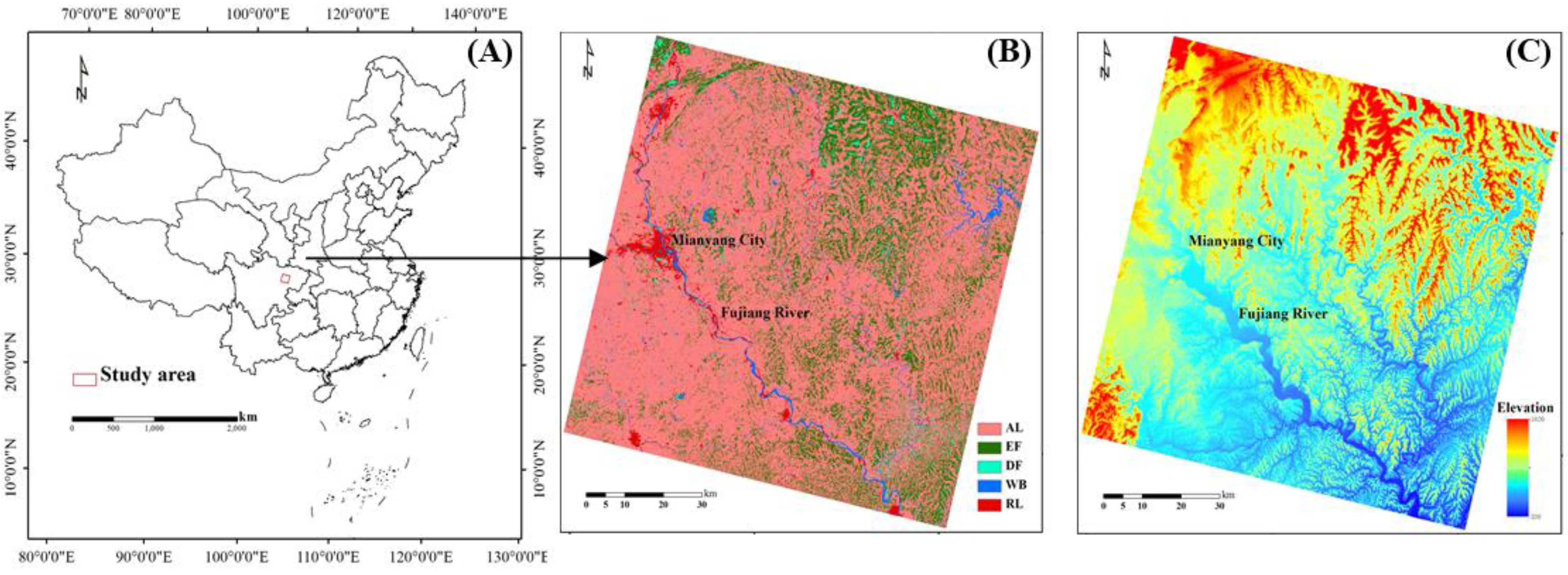
An area of about 8100 km2 (90 km × 90 km) in the eastern Sichuan province was selected as the case region (Figure 1A). The region is a typical hilly area with a high spatial heterogeneity of land cover (Figure 1C) and many types of surface features, among which farmland and forestland are the most widely distributed (Figure 1B). Mianyang, the second largest city in Sichuan, lies in the left middle of the area. The Fujiang River flows through the area from the northwest to the southeast (Figure 1B).

Figure 1.
(A) Location of the study area; (B) Land cover map of the study area; the abbreviation in the legend is defined as AL (arable lands), EF (evergreen forests), DF (deciduous forests), WB (water bodies), and RL (residential lands); (C) DEM of study area showing the terrain topography.
Figure 1.
(A) Location of the study area; (B) Land cover map of the study area; the abbreviation in the legend is defined as AL (arable lands), EF (evergreen forests), DF (deciduous forests), WB (water bodies), and RL (residential lands); (C) DEM of study area showing the terrain topography.
The area is located in the zone of the Sichuan Basin subtropical moist monsoon climate. The rainfall differs in the dry season and the wet season. It takes more than 80% of the annual rainfall capacity in the wet season (approximately from May to October) [19]. The temperature differs obviously in the four seasons: it is highest in summer, about 25 °C, moderate in spring and autumn, about 16–17 °C, and lowest in winter, only about 6 °C [20]. The pleasant climate allows a multiple-cropping system. The summer cropping season is approximately from May to October, and the winter cropping season is approximately from November to May of the next year. The types of vegetation are complex, the landscapes are fragmentary, and the farmlands are widely distributed and multiple cropping is common in the study area. With these features, the area is very suitable for the comparative analysis on the difference between the two different synthesizing schemes.
3. Data and Preprocessing
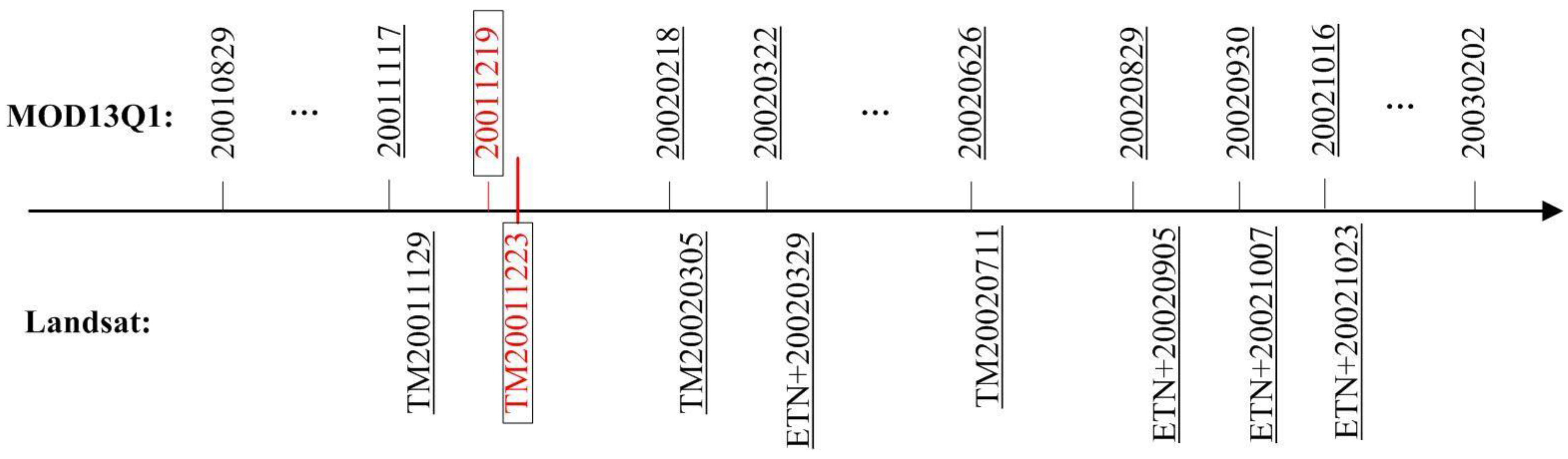
High quality Landsat images are needed to assess the prediction accuracy of the two schemes in this paper; while Landsat ETM+ images since May of 2003 are not suitable for validation due to the ill-scanned lines, seven Landsat TM or ETM+ scenes with little or no cloud during 2001 and 2002 were used as the experiment data (see Figure 2). In order to minimize the negative influence from cloud and shadow, the MODIS 16-day optimum observation composites (i.e., MOD13Q1) were selected as the high temporal resolution data. The dataset contains 12 layers in total. Only the red, the NIR, the NDVI, and the pixel reliability layers were selected in our study. As seen in Figure 2, the Landsat TM image on 23 December 2001 and the 23rd composite of MOD13Q1 data in 2001, corresponding to the TM image, were selected as the base images in the STARFM algorithm. The other 33 composites of MOD13Q1, from the 16th composite of 2001 to the third composite of 2003, were used as the input data with the 16-day temporal resolution. Because it requires additional adjacent data to eliminate the “edge effect” [21], the last seven composites of 2001 (i.e., the 16th to 22nd of 2001) and the first three composites of 2003 (i.e., the first to third of 2003) were also selected, beside all composites from 2002 (shown in Figure 2). All Landsat and MODIS data were downloaded from USGS GLOVIS portal website [22].
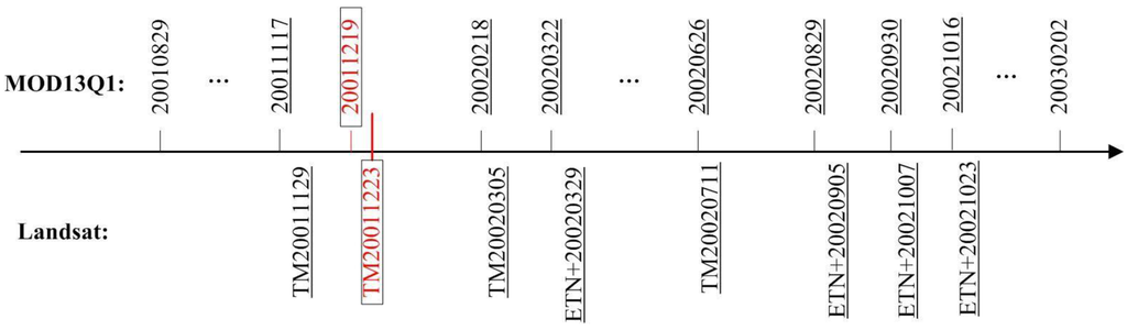
Figure 2.
Acquisition dates of Landsat and MODIS scenes used for this study. The Landsat image at base date (23 December 2001) and the corresponding MOD13Q1 image at base date (the 23rd composite in 2001) are marked with red squares. The reference Landsat images for validation and their corresponding MOD13Q1 images are marked with underlines. Note that MODIS data were acquired as 16-day composites; the dates given in the figure are the first day of the 16-day acquisition period respectively.
The projections and pixel sizes of the input Landsat and MODIS data must be same in the STARFM algorithm. Projection transformation, re-sampling, and cutting were done for MOD13Q1 products by the MRT (MODIS Reprojection Tool) to acquire 30 m-data with UTM projection. The LEDAPS procedure (i.e., Landsat Ecosystem Disturbance Adaptive Processing System) [23] was first utilized for radiometric calibration and atmosphere correction for Landsat data. Additionally, the surface reflectance and NDVI data were finally obtained from the preprocessed Landsat data.
A land cover map from 2000 was also applied for masking farmland while extracting crop information. The independent field validation showed that the accuracy of the land cover product surpassed 85%, which can meet the requirement of this study [24].
4. Methods
4.1. The STARFM Algorithm
As MODIS surface reflectance and Landsat surface reflectance are in high coincidence [25], if the MODIS surface reflectance is known at date t0 when the Landsat surface reflectance is unknown, the Landsat surface reflectance at t0 can be expressed as:
where (xi, yj) indicates a given pixel location for both Landsat and MODIS images; ε0 indicates the difference between MODIS surface reflectance and Landsat surface reflectance caused by different bandwidth and solar geometry.
If both the MODIS and Landsat surface reflectance at another date tk are known, under the assumed precondition that the land cover and the system error do not change from t0 to tk (i.e., ε0 = εk), the unknown Landsat surface reflectance at t0 can be evaluated by the following equation [9]:
In consideration of the mixed-pixel effect, land cover or phenological change, and the solar geometry bidirectional reflectance distribution function (BRDF), by introducing the information of similar neighbor pixels in a searching window, the unknown Landsat reflectance of the center pixel (xω/2, yω/2) at t0 can be expressed as:
where ω indicates the searching window size; and Wijk indicates the weight of similar neighbor pixels in a window, determined by the following three factors: (1) the spectral distance (Sijk) between Landsat and MODIS data at a given location at tk; (2) the spatial distance (dijk) between a neighbor pixel and the central pixel; and (3) the time distance (Tijk) between the input and the predicted MODIS data.
The condition for filtering similar neighbor pixels in a window is that it must provide more spectral and spatial information than the central pixel. An uncertainty parameter is added to the filtering condition, in consideration of the uncertainty during the preprocessing procedures for Landsat and MODIS surface reflectance. The original literature could be referred to for more detailed descriptions of the calculation methods of all parameters and the algorithm theory [9].
4.2. Two Comparable Schemes
Theoretically, there are two different schemes for synthesizing HTSNs based on the STARFM algorithm. They are described as follows.
Scheme 1: Taking the test data introduced in Section 3 as an example, high temporal Landsat-like red and NIR reflectance images can be generated by using the TM image from the 23 December 2001 and time-series MOD13Q1 dataset by the STARFM algorithm, and then the high temporal Landsat-like NDVI data can be indirectly obtained through algebraic operation (Figure 3A).
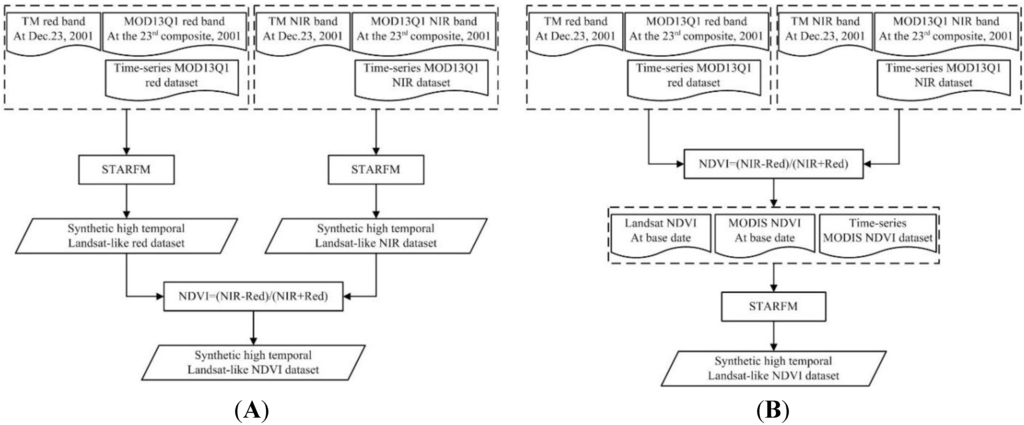
Figure 3.
The flowchart of Scheme 1 (A) and Scheme 2 (B) for synthesizing the HTSNs.
Figure 3.
The flowchart of Scheme 1 (A) and Scheme 2 (B) for synthesizing the HTSNs.

Scheme 2: First, all the reflectance images, including those in TM and MOD13Q1, are used to figure out the NDVI images, and then the high temporal Landsat-like NDVI data can be synthesized directly by fusing the derived NDVI images through the STARFM algorithm (Figure 3B).
4.3. Parameter Settings
For the STARFM algorithm, it is recommended that different parameter combinations should be used for regions with different spatial heterogeneity. The sliding window size should be set bigger, and a logarithmic formula that is insensitive to spectral distance should be applied for calculating the weights of similar neighbor pixels for regions with high heterogeneity [9]. Simultaneously, the uncertainty parameter should also be set according to the spatial heterogeneity and the fluctuation range of one band value. For regions with high spatial heterogeneity, the uncertainty of the red band is usually set as 0.01, and that of the NIR band is set as 0.015 [9]. In this study, in consideration of the fact that the study area is a hilly area with high spatial heterogeneity, the sliding window size was set as 3000 m × 3000 m. As the NDVI band fluctuates wider than the NIR band does, the uncertainty parameter of the NDVI band was set as 0.025.
4.4. Comparison and Evaluation Protocol
4.4.1. Prediction Accuracy Evaluation
Taking the acquired Landsat TM or ETM+ images as the validation data, the general prediction accuracy of different schemes can be compared with each other. The observed Landsat images and their corresponding predicted Landsat-like images were applied to figure out the determination coefficient (R2) and RMSE (root mean square error), which were taken as the evaluation indexes to evaluate the prediction accuracy of different schemes. Because MOD13Q1 data are composed in a 16-day period, the observed Landsat images cannot exactly coincide with the predicted Landsat-like images in terms of time. The date span of MOD13Q1 data and its corresponding predicted Landsat-like image should cover the observation date when the actual Landsat image was acquired. For example, the predicted Landsat-like image corresponding to the 21st composite of MOD13Q1 in 2001 was selected and compared with the acquired TM image from 29 November 2001 because the composite dates of the MOD13Q1 (i.e., from 17 November to 2 December 2001) included the observation date of the actual TM image (i.e., 29 November 2001). Furthermore, the prediction accuracies of the red band and NIR band were also calculated along with the NDVI band for Scheme 1, while only the prediction accuracy of the NDVI band was calculated for Scheme 2.
4.4.2. Consistence Comparisons
Two HTSNs synthesized by two different schemes were compared with each other from temporal and spatial domains:
Temporal Consistence: The correlation coefficient R between the two same temporal NDVI images from two synthesized HTSNs was calculated, and a temporal curve of R was then laid out for presenting the temporal consistence between the two HTSNs (illustrated as Figure 4A).
Spatial Consistence: The correlation coefficient R between the two time-series NDVIs extracted from two synthesized HTSNs was calculated for each pixel; then a spatial map of R for all the pixels was figured out and was used for describing the spatial consistence between the two HTSNs (illustrated as Figure 4B).
4.4.3. Application Comparisons
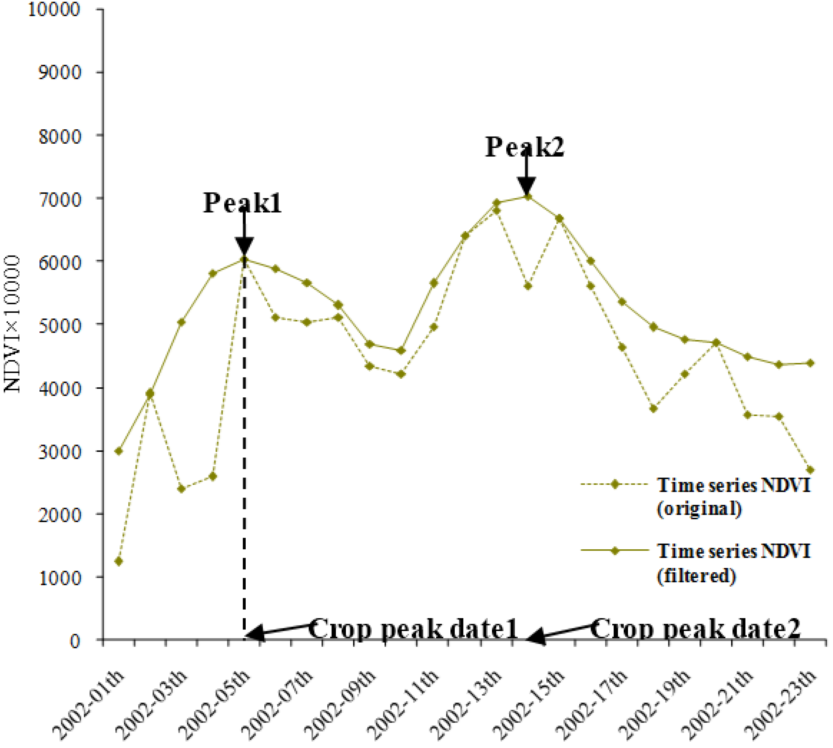
Time-series NDVI data are often used to extract important farming information like cropping intensity and crop phenology [26,27]. It was found that the peak of the time-series NDVI curve indicated that the ground biomass of crops reached the maximum and fluctuated with the crop-growing processes such as sowing, seeding, heading, ripeness, and harvesting within one year [28]. Correspondingly, cropping intensity is defined as the number of peaks and the crop peak date is defined as the timing when the emerging “peak” is in the time-series NDVI curve (Figure 5). In this paper, application comparisons were carried out for extracting the cropping intensity and the crop peak dates in the study area based on two HTSNs synthesized by two different schemes. Two results for the same application were compared with each other pixel by pixel. The coincidence rate, the percentage of the pixels whose results based on both HTSNs is exactly the same, was figured out for presenting the difference between them. An analysis was then made to determine whether the difference between the two HTSNs would cause a significant impact on such applications.
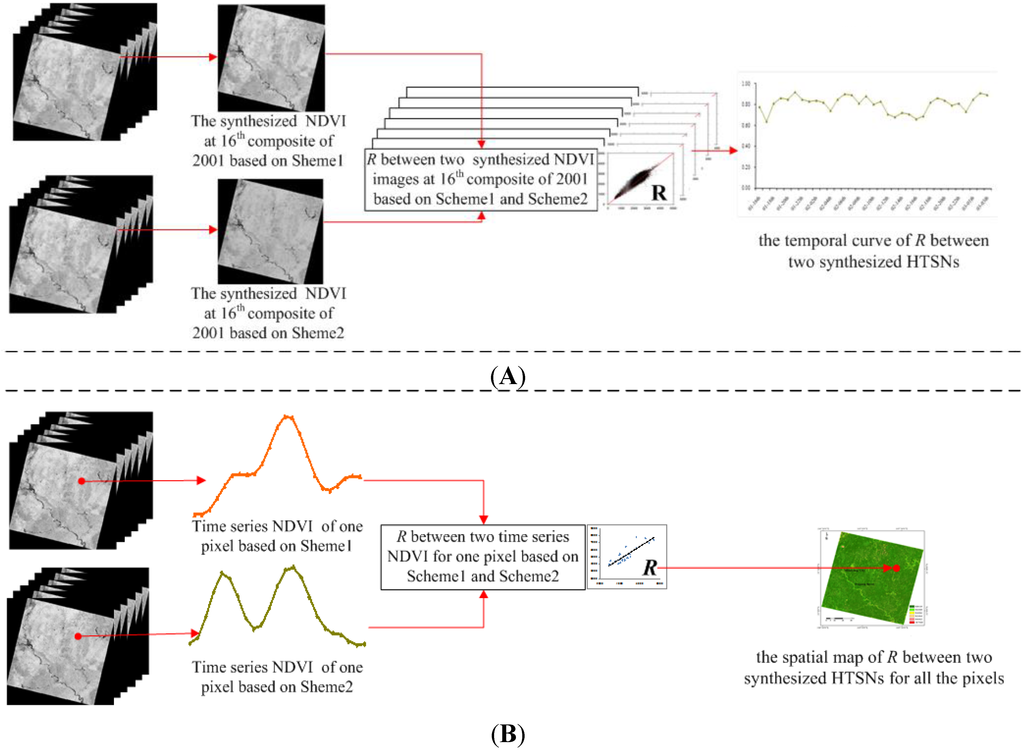
Figure 4.
The illustrations for describing the temporal consistence and the spatial consistence between two HTSNs synthesized by two different schemes. (A) Temporal correlation: taking the 16th composite in 2001 as an example, the correlation coefficient R between the two synthesized NDVI images at the composite was calculated; the value was a point of the temporal curve of R between the two synthesized HTSNs; (B) Spatial correlation: taking one pixel as an example, two time-series NDVI values for the pixel were extracted, and the correlation coefficient R between them was calculated; the value was a point of the spatial map of R between two synthesized HTSNs for all the pixels.

Two synthesized HTSNs were first filtered by the S-G filter [21,29] in order to eliminate the negative effect from clouds and shadows (see Figure 5). Possible peaks were then extracted by the second order difference algorithm [30,31], and the “fake peaks” were kicked out by the test conditions of the peak emerging date and the threshold of the peak value. The test conditions were set as the dates of crop peaks that should emerge within the potential crop growth seasons (see above Section 2), and the NDVI value of peaks should be more than 0.4. Subsequently, the cropping intensity was acquired through counting the number of peaks, and the date of each peak was simultaneously recorded. While extracting the cropping intensity and crop peak dates, the results were masked for the farmland using the land cover product.
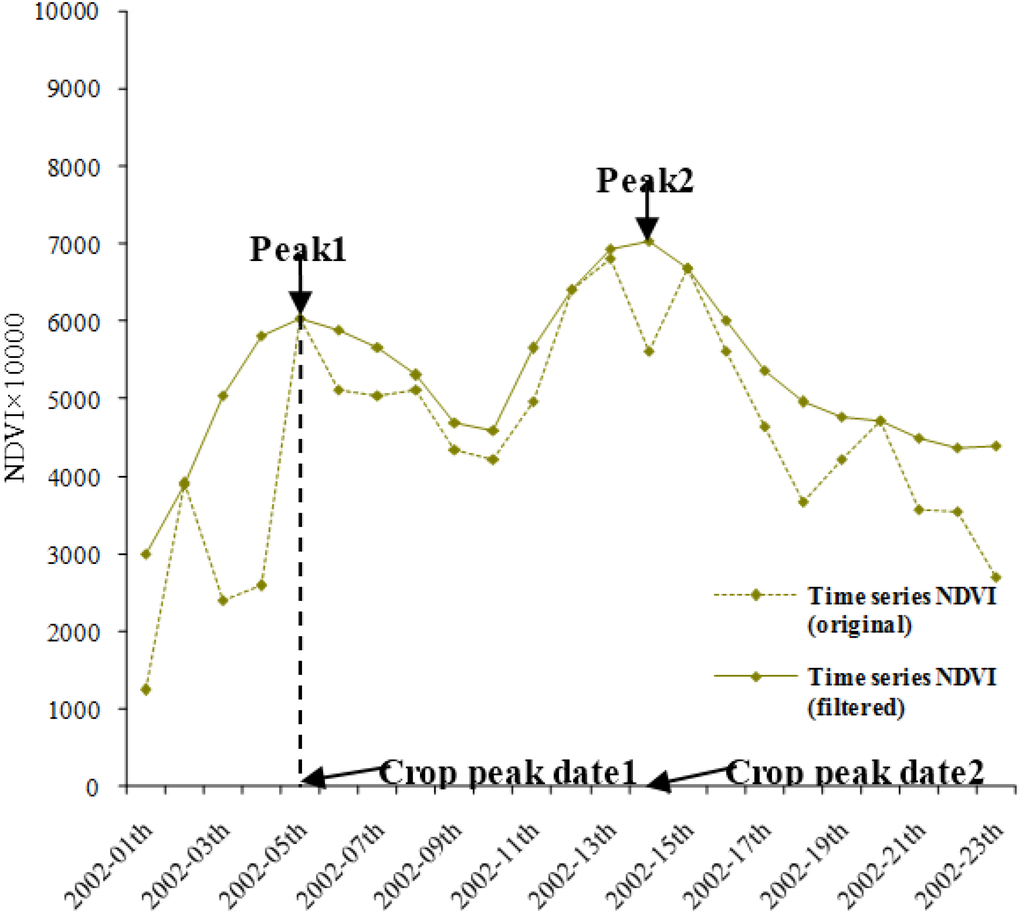
Figure 5.
The illustration for presenting cropping intensity and crop peak dates in the study. The 2002-01th on the horizontal axis indicates the first composite in 2002, and so on.
Figure 5.
The illustration for presenting cropping intensity and crop peak dates in the study. The 2002-01th on the horizontal axis indicates the first composite in 2002, and so on.
5. Results and Analysis
5.1. Prediction Accuracy Comparisons
For seven acquired Landsat images (listed in Figure 2), R2 and RMSE between the actual Landsat images and the predicted images by the two different schemes are described in Table 1. The prediction accuracy of both schemes is similar. Scheme 2 is slightly superior to Scheme 1. Comparably, the NDVI prediction accuracies of both schemes are in good agreement (R2: 0.14 < Scheme 1 < 0.53; 0.15 < Scheme 2 < 0.53), while the predictions of dates on 5 March 2002 and on 5 September 2002 are relative poor. Generally, rape blooms in the beginning of March and corn and rice mature gradually in the beginning of September. Thus, high heterogeneity exists in space at the two moments, which may lead to worse predictions according to the characteristics of the STARFM algorithm [9]. Similarly, the predictions of dates on 29 November 2001 and on 29 March 2002 are comparatively good (Table 1), likely because rape grows few leaves at the end of November or is close to the peak of the growing season at the end of March, when high homogeneity exists. For Scheme 1, the prediction accuracies on the three bands (i.e., red, NIR, and NDVI) are different from each other.
5.2. Consistence Comparisons
5.2.1. Temporal Consistence
The temporal curve of R between the two synthesized HTSNs is presented in Figure 6. The two HTSNs show fairly high temporal consistence in general, and most of the correlation coefficients are above 0.8, some even above 0.9. The composites with the high correlation coefficients are decentralized in all seasons except summer. Furthermore, the highest correlation coefficients are respectively corresponding to the 21st composite of year 2001 (winter, R = 0.92), the second composite of 2003 (winter, R = 0.91), and the sixth composite of 2002 (spring, R = 0.90) (see the black arrows in Figure 6). The composites with comparatively lower correlation are concentrated, mostly from the 12th to the 17th, in the summer of 2002 (0.66 < R < 0.72, the acquisition dates from 26 June to 29 September 2002; see the red arrows in Figure 6).

Table 1.
Results of the pixel-based regression of the reference Landsat images versus the predicted images by two schemes for seven acquisition dates. The better result for each date is shown in bold.
| Acquisition Dates (MM-DD-YYYY) | R2 | RMSE | ||||||
|---|---|---|---|---|---|---|---|---|
| Scheme 1 | Scheme 2 | Scheme 1 | Scheme 2 | |||||
| Red | NIR | NDVI | NDVI | Red | NIR | NDVI | NDVI | |
| 11-29-2001 | 0.42 | 0.72 | 0.42 | 0.46 | 0.02 | 0.03 | 0.10 | 0.09 |
| 03-05-2002 | 0.01 | 0.42 | 0.14 | 0.15 | 0.07 | 0.06 | 0.29 | 0.30 |
| 03-29-2002 | 0.64 | 0.67 | 0.53 | 0.53 | 0.02 | 0.04 | 0.09 | 0.10 |
| 07-11-2002 | 0.32 | 0.45 | 0.30 | 0.36 | 0.02 | 0.07 | 0.09 | 0.11 |
| 09-05-2002 | 0.45 | 0.42 | 0.23 | 0.15 | 0.02 | 0.07 | 0.10 | 0.11 |
| 10-07-2002 | 0.45 | 0.29 | 0.23 | 0.27 | 0.02 | 0.05 | 0.11 | 0.12 |
| 10-23-2002 | 0.56 | 0.36 | 0.28 | 0.29 | 0.02 | 0.04 | 0.13 | 0.13 |
5.2.2. Spatial Consistence
Figure 7 shows the spatial map of R between two synthesized HTSNs. The spatial consistence between them is fairly high, with R above 0.8 at most areas (see Figure 7A), but it still reveals some difference in space. In contrast to the land cover map, the spatial map is seemingly associated with the land cover types (Figure 7A vs. Figure 7B). The spatial correlation at farmlands is fairly high, with the mean R of 0.91. The correlation at forestlands takes second place (b1 and b2 in Figure 7), with the average R of 0.86. While R at water body regions (e.g., α and β in Figure 7) is comparatively low, and even negative in areas of residence zones (see a1 vs. b1 in Figure 7)).
The nonlinear relation between the NDVI band, red band, and NIR band may explain the spatiotemporal characteristics mentioned above. The larger the obvious nonlinear relation that exists, the bigger the difference between the two HTSNs will be, and the results will be in lower correlation. The temporal curve of R tends to be low in the summer (shown in Figure 6), likely because crops or vegetation grow prosperously in summer when the NDVI can reach fairly high values and the obvious nonlinear relation exists between the NDVI band, red band, and NIR band [18]. Similarly, the spatial map of R shows low values in water body and residence areas (see Figure 7), likely because the NDVI values in those areas are fairly low and the obvious nonlinear relation also exists [18]. Additionally, following the spatiotemporal characteristics, two results based on the two HTSNs in the same application in farmlands or forests may have little difference, since the two HTSNs in those areas shows higher spatial consistence. However, more attention should be paid when the summer season is considered for comparisons of the two results, just because the two HTSNs show lower temporal consistence in summer.
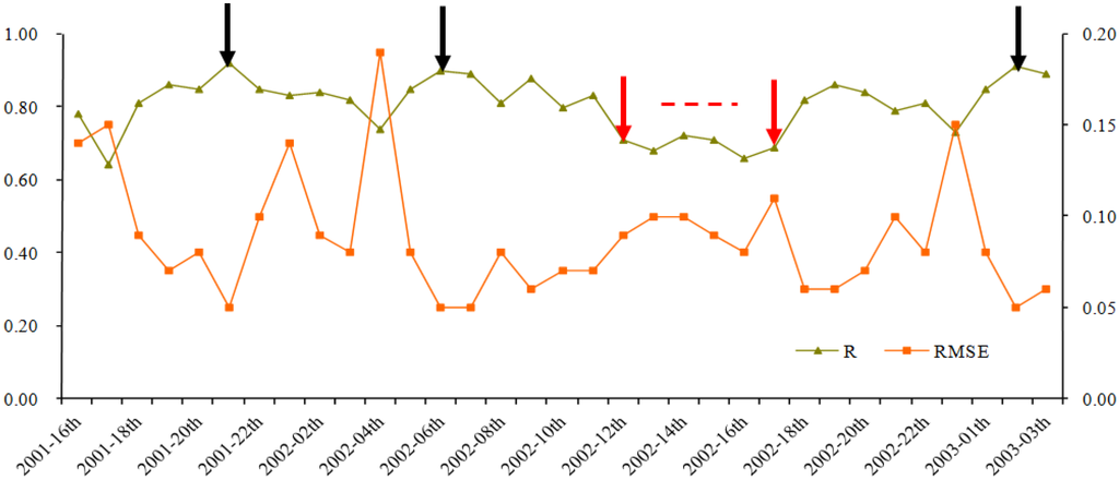
Figure 6.
The temporal curve of R between two HTSNs synthesized by two different schemes. Three composites with high correlation coefficients are decentralized in all seasons except summer. The highest correlation coefficients marked with black arrows above 0.9 are respectively corresponding to the 21st composite of 2001 (winter, R = 0.92), the second composite of 2003 (winter, R = 0.91), and the sixth composite of 2002 (spring, R = 0.90). The lower correlation coefficients marked with red arrows are corresponding to the 12th through the 17th composites in summer of 2002.
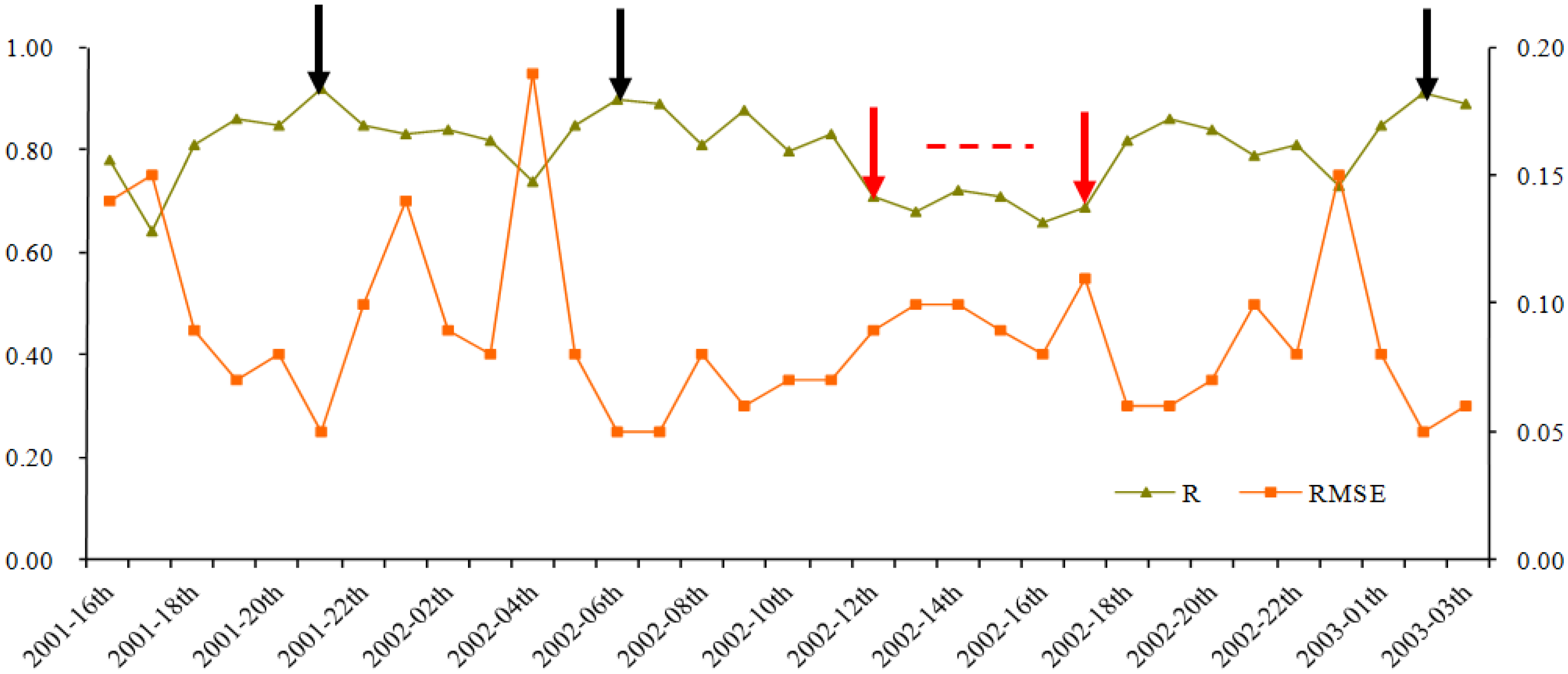
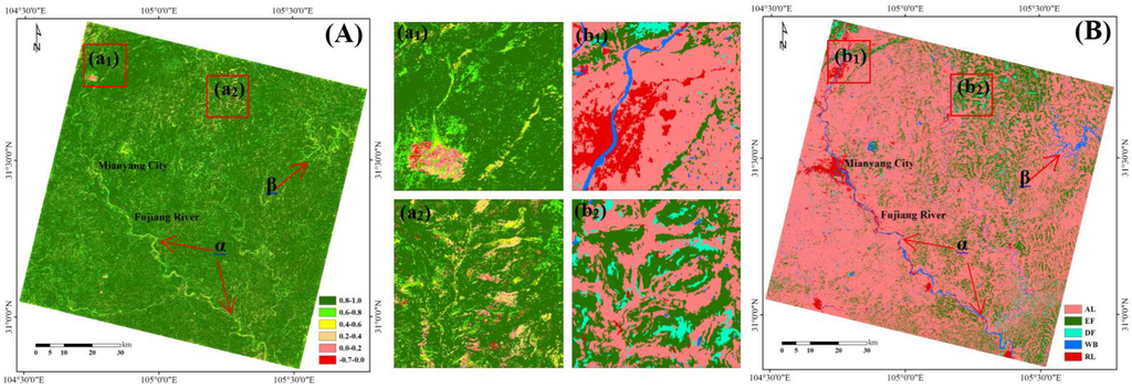
Figure 7.
The spatial map of R between two HTSNs synthesized by two different schemes, (A) for the spatial map of R and (B) for the land cover map. The legend in (B) is same as that in Figure 1B.
Figure 7.
The spatial map of R between two HTSNs synthesized by two different schemes, (A) for the spatial map of R and (B) for the land cover map. The legend in (B) is same as that in Figure 1B.

5.3. Application Comparisons
5.3.1. Cropping Intensity
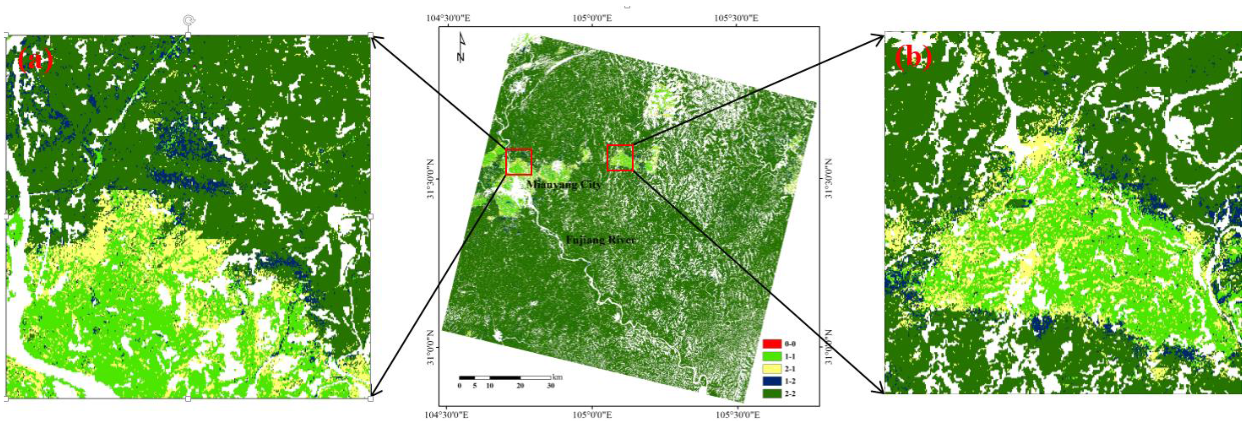
The statistics on the comparisons of cropping intensity extracted from the two HTSNs are listed in Table 2. The fallow pixels have low coincidence, being only 20.57%. However, the result has no statistical significance, as the numbers of fallow pixels extracted under both schemes are small (1810 pixels in Scheme 2 and only 1118 pixels in Scheme 1). Therefore, no further analysis is made on the fallow. For the pixels extracted on the single cropping system, the coincidence rate is low, only reaching 56.81%. From the pixel-by-pixel comparison map (Figure 8), it can be discovered that the nonconformity is mainly found in part of the transitional zone between the single cropping system and the double cropping system (Figure 8). The main reason for this inconformity is that the judgment of “whether the first crop has been cultivated” is different based on the two proposed schemes upon further inspection. It may be related to the complex spatial distribution of crops in the period. The single-cropping farmlands are mostly used for planting autumn grain crops in the area. Weeds would grow on the farmlands when there is no plantation. At the same time, summer grain crops grow on the double-cropping farmlands. The HTSNs in the transitional zone may be affected by either the weeds on the single-cropping farmlands or the summer grain crops on the double-cropping farmlands for the farmlands in the transitional zone. Thus, the judgments based on the HTSNs would be “the first crop has not been cultivated” impacted on the former, or “the first crop has been cultivated” impacted on the latter, finally resulting in that the cropping intensity results are usually different. However, the result for the pixels of the double cropping system is very high, reaching up to 96.12%, which is obviously consistent with the comparison map (Figure 8). Overall, the cropping intensity results of the two schemes generally coincide with each other fairly well, reaching up to 93.86%.
Table 2.
The statistics of comparisons in the results of cropping intensity and crop peak dates based on two HTSNs synthesized by two different schemes. The numbers in the table indicate the number of 30 m pixels.
| Cropping System | Cropping Intensity | Crop Peak Date | ||||
|---|---|---|---|---|---|---|
| Coincidence | Total a | Coincidence Rate b | Coincidence | Total a | Coincidence Rate b | |
| No-till | 230 | 1118 | 20.57% | - | - | - |
| Single crop | 283,618 | 499,273 | 56.81% | 176,034 | 499,273 | 35.26% |
| Double crops | 7,933,397 | 8,253,983 | 96.12% | 11,890,458c | 16,507,966 c | 72.03% |
| All | 8,217,245 | 8,754,374 | 93.86% | 12,066,492 | 17,007,239 | 70.95% |
Note: Total a is the number of the pixels in different cropping systems (i.e., no-till, single crop, or double crops) based on Scheme 2; Coincidence rate b is the percentage of the pixels whose results of cropping intensity based on Scheme 2 are the same as Scheme 1; the superior character c means that as the coincidence rate of the first crop and the second crop in the double cropping system are calculated respectively, the total number of pixels in double crops is 16,507,966 (8,253,983 × 2).

Figure 8.
Comparison map between the results of cropping intensity based on two HTSNs synthesized by two different schemes. The former of the “x-x” in the map legend indicates the result of Scheme 1, and the latter indicates the result of Scheme 2. For example, 2-1 indicates that the result for Scheme 1 is 2, while that for Scheme 2 is 1.
5.3.2. Crop Peak Date
The statistical results of the coincidence rate of crop peak dates extracted from two HTSNs are showed in Table 2. Compared to the results of cropping intensity, both coincidence rates of the crop peak dates are fairly low. Especially for the single cropping system, the coincidence rate is only 35.26%. This may be because the spatial distribution of single-cropping farmlands is fragmentation and their growing season supersedes with the double-cropping farmlands in time. Such superseding may cause that the peak date of the crop in single cropping system appear in advance influenced by the first crop in double cropping system, or that it may delay influenced by the second crop in double cropping system. For the double cropping system, the coincidence rate is also not very high, about 72.03%. In general, the coincidence rate for extracting crop peak date is about 70.95%, which is far lower than that of extracting cropping intensity.
6. Discussions
6.1. Parameter Settings
According to the STARFM algorithm, three parameters (including sliding window size, uncertainty, and weighting strategy) are decisive for the predictions. The former two parameters determine how many and which pixels need to be involved as similar neighbor pixels in the prediction procedure, and the last one determines the contribution of candidate pixels to the central pixel in the window. Although the sliding window size was set as 1500 m in most of studies, the findings showed that such a setting did not always obtain good predictions in different regions. If the window size is set too big, more neighbor pixels would participate in the prediction procedure, resulting in predicted images that are vague [17]; however, if the window size is set too small, it may be difficult to find enough “pure” pixels, causing the prediction accuracy to be low [9]. The setting of uncertainty also encounters such a problem. One of the solutions is to observe some prediction results with different parameter combinations by series experiments so that one suitable parameter combination for a region can be obtained. The different weighting strategies for neighbor pixels also have some impact on the predicted results [17]. The setting for the weighting strategies was fairly simple and the mechanism was not fully considered in the original algorithm. An improvement has been made in the calculation of the spectral weight through the simple classified statistic method [32]. If the internal relations between similar neighbor pixels in the study area can be found through geo-statistical methods, it may be more helpful for the optimization of the weighting strategies. While the applications of the STARFM algorithm are developing gradually in other fields, it is a more reasonable strategy to change the filtering method and the weighting strategy for similar neighbor pixels, according to the characteristics of the mechanism itself in specific applications [33,34].
6.2. Prediction Accuracy
Similar to the previous research on constructing high temporal and spatial resolution data based on the STARFM algorithm, taking farmland as the main area [11,35], the correlations between the predicted images and the observed images at the red band and NIR band are both verified on the low side (R2: 0.01–0.72) in this paper. For the hilly area in eastern Sichuan where the terrain is comparatively complex, the crop structure on farmland is easily disturbed by human activity and the spatial heterogeneity is fairly high. It may potentially cause the correlation between the prediction values and the real values to be lower. Comparably, in some research taking forests or shrubs as the main area, there were better correlations between the predicted images and the observed images [12,15,16,36,37], due to the low spatial heterogeneity of the surface features. Therefore, combining specific applications such as crop phenology monitoring, it still requires the evaluation of how accurate and useful the synthesized time-series Landsat-like NDVI data are when used in practical applications. As this is not the main objective of this paper, no further discussion is carried out about this issue.
Because the shorter wavelength bands are more easily affected by the atmosphere condition [38], the verified correlation of the NIR band is generally superior to that of the red band (Table 1). This is the same as the results of some related research [11,15,35]. However, some other researchers showed totally opposite results [16,36]. The possible reason was analyzed in Walker et al. [36] who showed that the Landsat images in their research were not corrected for the view angle effects while the MODIS images were NBAR data-corrected for solar- and view- angle. Such differences can be amplified in areas where there are multiple layers of tall vegetation cover because these areas would cause higher scattering of the NIR band. Therefore, in areas where the number of layers of vegetation cover is few or the height of vegetation is low (e.g., farmland), the correlation of the NIR band is still superior to that of the red band.
In the prediction of three bands (red, NIR and NDVI) in Scheme 1, the verified correlations of the NDVI band are lower than those of the red and NIR bands (Table 1). It is discovered that the correlation of the NDVI band is slightly lower than those of the red and NIR bands in dry land and forest areas [12], while the result is completely opposite in forest areas in temperate zones [15]. If NDVI can be deemed as a band with a longer wavelength than the NIR band, the reason for this difference may be the different atmosphere conditions in the research areas. In the research area of Hilke et al. [15], compared to NDVI, the red and NIR bands with shorter wavelength are more easily affected by the atmosphere conditions [12]. Comparing the predicted results of the two schemes on the NDVI bands with each other, Tian et al. [37] declared that the verified correlation of Scheme 2 is obviously superior to that of Scheme 1. The likely explanation is that the effect of atmosphere is further reduced after the red band and NIR band are used to calculate the NDVI band. However, it is worth noticing that the results in this paper show that Scheme 2 is only slightly superior to Scheme 1. The main surface cover is shrubs in Tian et al.’s research area, where the high NDVI value in the growing season may be often saturated. Thus, the difference between the two schemes is amplified because of the more obvious nonlinear relation at high values. However, the NDVI is often at medium values even in the growing season of crops, and the nonlinear relation is not obvious in such areas [18]. As a result, there is little difference between the predicted results of Scheme 1 and Scheme 2 in this paper.
6.3. Applications
Small differences exist between the two HTSNs, though they are generally in good agreement (Table 1, Figure 6 and Figure 7). However, such differences have very different effects on different specific applications. The results of the experiment show the application of extracting cropping intensity is not sensitive to such differences. The coincidence rate of such an application between two synthesized HTSNs is about 93.86%. Since the high coincidence rate means that it gets almost the same results of extracting cropping intensity based on two different schemes, Scheme 2 can then be considered an alternate scheme for Scheme 1, so that more time and memory space can be saved, because only one band (i.e., NDVI) is operated in Scheme 2. Especially for the hilly areas, existing research demonstrated that the time-series NDVI with coarse spatial resolution (e.g., MODIS) cannot get satisficatory accuracy for retrieving the cropping intensity [30,39]. Such a design (i.e., Scheme 2 instead of Scheme 1) will be very useful for generating the HTSNs, which may improve the accuracy. However, the application of recording crop peak dates is very sensitive to the difference. The coincidence rate of that application between the two schemes is only about 70.95%. It should be noted that the MODIS data synthesized to the HTSN is a composite of 16-day optimum observations, which means that, in fact, the difference may be 0 to 32 day(s) between the two results of crop peak dates for one pixel. Thus, the coincidence rate may be lower, if the temporal scale is decreased to eight days or less. Therefore, for more quantitative applications such as extracting the crop peak dates, Scheme 2 cannot be used to replace Scheme 1 because of the low coincidence rate. Their absolute accuracy should be compared with ground observations in subsequent research in order to judge which scheme is more suitable for extracting crop peak date information.
Besides, as the spatial consistence between the two HTSNs in shrub lands is lower than that in farmlands, careful execution is needed when selecting a scheme for these areas. Although existing research shows that the prediction accuracy of Scheme 2 is superior to Scheme 1 in bush areas [37], it cannot be inferred that Scheme 2 is still superior to Scheme 1 in specific applications. In the follow-up research, more reliable verification data (e.g., the ground measurement data) are needed to compare the application effect of the two schemes.
7. Conclusions
The STARFM algorithm was popularly used for synthesizing the surface reflectance as well as NDVI with high temporal and spatial resolutions. As mentioned in the paper, there are two different schemes for synthesize the NDVI dataset with high temporal and temporal resolutions (HTSN) through the STARFM algorithm. Two HTSNs based on the two schemes were compared with each other in this paper. Selecting the hilly area in eastern Sichuan province of China as the research area, seven scenes of Landsat images and time-series MOD13Q1 spanning from October 2001 to February 2003 were chosen as test data. The comparison results showed that the different procedures in the two schemes did not greatly influence the synthesized time-series Landsat-like NDVI dataset. In general, the prediction accuracies of both HTSNs are almost the same (R2: 0.14 < Scheme 1 < 0.53; 0.15 < Scheme 2 < 0.53), and the two HTSNs are high in temporal and spatial consistence. However, different applications presented different sensitivities to the small spatiotemporal difference between them, judging from the fact that the results were significantly different when the two HTSNs were applied in applications of extracting cropping intensity and crop peak dates. In the case of extracting cropping intensity, there was a fairly high coincidence rate, reaching up to 93.86%; however, in the case of extracting the crop peak dates, the coincidence rate was low at only 70.95%. Therefore, it is believed in this paper that Scheme 2 (i.e., the NDVI band is directly inputted to the STARFM) can replace Scheme 1 in the application of extracting cropping intensity in order to save more time and memory space because Scheme 2 requires only one band input (i.e., NDVI).
The HTSN is needed urgently for obtaining agricultural information in areas with a complex earth surface. In addition to selecting suitable algorithms for synthesizing the HTSN, it is also necessary to compare different schemes based on the same algorithm. For the STARFM algorithm, considering that Scheme 2 requires a shorter time and smaller memory space and that it is easier to obtain the NDVI dataset with it compared with surface reflectance data, the research result of this paper provides evidence for synthesizing the HTSN in complex surface areas in a simpler way and for further extracting the cropping intensity information of farmland. However, for more quantitative applications such as extracting the crop peak dates, the low general coincidence rate means that fairly different results may come out based on the two HTSNs. Therefore, it is necessary to compare the absolute accuracy of both schemes in subsequent research in order to select which scheme is better for extracting the phenological information of crops.
Acknowledgments
The authors wish to express their gratitude to the Landsat Science Team and the MODIS science team for the excellent and accessible data products. This research was supported jointly by the key projects of CAS (Grant No. KZZD-EW-TZ-06, GJHZ201320 and XDA05050105), and the National Natural Science Foundation project of China (41271433). We are grateful to the anonymous reviewers whose constructive suggestions will be useful for improving the quality of our manuscript.
Author Contributions
All authors have made major and unique contributions. Ainong Li designed the framework of this research work, and finished the final version of this paper. Wei Zhang performed the data generation, data validation analysis, results interpretation. Guangbin Lei took part in data analysis, results interpretation. Jinhu Bian performed the data collection and preprocessing.
Conflicts of Interest
The authors declare no conflict of interest.
References
- Marfai, M.A.; Almohammad, H.; Dey, S.; Susanto, B.; King, L. Coastal dynamic and shoreline mapping: Multi-sources spatial data analysis in Semarang Indonesia. Environ. Monit. Assess. 2008, 142, 297–308. [Google Scholar] [CrossRef] [PubMed]
- Hilker, T.; Wulder, M.A.; Coops, N.C.; Linke, J.; McDermid, G.; Masek, J.G.; Gao, F.; White, J.C. A new data fusion model for high spatial-and temporal-resolution mapping of forest disturbance based on Landsat and MODIS. Remote Sens. Environ. 2009, 113, 1613–1627. [Google Scholar] [CrossRef]
- Arai, E.; Shimabukuro, Y.E.; Pereira, G.; Vijaykumar, N.L. A multi-resolution multi-temporal technique for detecting and mapping deforestation in the Brazilian Amazon rainforest. Remote Sens. 2011, 3, 1943–1956. [Google Scholar] [CrossRef]
- Zhang, W.; Li, A.; Jin, H.; Bian, J.; Zhang, Z.; Lei, G.; Qin, Z.; Huang, C. An enhanced spatial and temporal data fusion model for fusing Landsat and MODIS surface reflectance to generate high temporal Landsat-like data. Remote Sens. 2013, 5, 5346–5368. [Google Scholar] [CrossRef]
- Maselli, F. Definition of spatially variable spectral endmembers by locally calibrated multivariate regression analyses. Remote Sens. Environ. 2001, 75, 29–38. [Google Scholar] [CrossRef]
- Busetto, L.; Meroni, M.; Colombo, R. Combining medium and coarse spatial resolution satellite data to improve the estimation of sub-pixel NDVI time series. Remote Sens. Environ. 2008, 112, 118–131. [Google Scholar] [CrossRef]
- Fischer, A. A simple model for the temporal variations of NDVI at regional scale over agricultural countries. Validation with ground radiometric measurements. Int. J. Remote Sens. 1994, 15, 1421–1446. [Google Scholar] [CrossRef]
- Kerdiles, H.; Grondona, M. NOAA-AVHRR NDVI decomposition and subpixel classification using linear mixing in the Argentinean Pampa. Int. J. Remote Sens. 1995, 16, 1303–1325. [Google Scholar] [CrossRef]
- Gao, F.; Masek, J.; Schwaller, M.; Hall, F. On the blending of the Landsat and MODIS surface reflectance: Predicting daily Landsat surface reflectance. IEEE Trans. Geosci. Remote Sens. 2006, 44, 2207–2218. [Google Scholar]
- Zurita-Milla, R.; Kaiser, G.; Clevers, J.; Schneider, W.; Schaepman, M. Downscaling time series of MERIS full resolution data to monitor vegetation seasonal dynamics. Remote Sens. Environ. 2009, 113, 1874–1885. [Google Scholar] [CrossRef]
- Watts, J.D.; Powell, S.L.; Lawrence, R.L.; Hilker, T. Improved classification of conservation tillage adoption using high temporal and synthetic satellite imagery. Remote Sens. Environ. 2011, 115, 66–75. [Google Scholar] [CrossRef]
- Walker, J.; De Beurs, K.; Wynne, R.; Gao, F. Evaluation of Landsat and MODIS data fusion products for analysis of dryland forest phenology. Remote Sens. Environ. 2012, 117, 381–393. [Google Scholar] [CrossRef]
- Schmidt, M.; Udelhoven, T.; Gill, T.; Röder, A. Long term data fusion for a dense time series analysis with MODIS and Landsat imagery in an Australian Savanna. J. Appl. Remote Sens. 2012, 6, 1–18. [Google Scholar]
- Emelyanova, I.V.; McVicar, T.R.; Van Niel, T.G.; Li, L.T.; Van Dijk, A.I. Assessing the accuracy of blending Landsat? MODIS surface reflectances in two landscapes with contrasting spatial and temporal dynamics: A framework for algorithm selection. Remote Sens. Environ. 2013, 133, 193–209. [Google Scholar] [CrossRef]
- Hilker, T.; Wulder, M.A.; Coops, N.C.; Seitz, N.; White, J.C.; Gao, F.; Masek, J.G.; Stenhouse, G. Generation of dense time series synthetic Landsat data through data blending with MODIS using a spatial and temporal adaptive reflectance fusion model. Remote Sens. Environ. 2009, 113, 1988–1999. [Google Scholar] [CrossRef]
- Bhandari, S.; Phinn, S.; Gill, T. Preparing Landsat Image Time Series (LITS) for monitoring changes in vegetation phenology in Queensland, Australia. Remote Sens. 2012, 4, 1856–1886. [Google Scholar] [CrossRef]
- Meng, J.; Wu, B.; Du, X.; Niu, L.; Zhuang, F. Method to construct high sptial and temporal resolution NDVI dataset-STAVFM. J. Remote Sens. 2011, 15, 44–59. (in Chinese). [Google Scholar]
- Wang, Z.; Liu, C.; Huete, A. From AVHRR-NDVI to MODIS-EVI: Advances in vegetation index research. Acta Eco. Sin. 2003, 23, 979–987. (in Chinese). [Google Scholar]
- Zhong, A.; Li, Y. Spatial and temporal distribution characteristics and variation tendency of Precipitation in Mianyang. Plate Mt. Meteor. Res. 2009, 29, 63–69. (in Chinese). [Google Scholar]
- The National Bureau of Statistics Survey Team in Mianyang City. The Bureau of Statistics of Mianyang City. In Statistical Yearbook of Mianyang City; China Statistics Press: Beijing, China, 2011; pp. 17–21. [Google Scholar]
- Chen, J.; Jönsson, P.; Tamura, M.; Gu, Z.; Matsushita, B.; Eklundh, L. A simple method for reconstructing a high-quality NDVI time-series data set based on the Savitzky–Golay filter. Remote Sens. Environ. 2004, 91, 332–344. [Google Scholar] [CrossRef]
- USGS Global Visualization Viewer. Available online: http://glovis.usgs.gov (accessed on 13 August 2015).
- Masek, J.G.; Vermote, E.F.; Saleous, N.E.; Wolfe, R.; Hall, F.G.; Huemmrich, K.F.; Gao, F.; Kutler, J.; Lim, T.-K. A Landsat surface reflectance dataset for North America, 1990–2000. IEEE Geosci. Remote Sens. Lett. 2006, 3, 68–72. [Google Scholar] [CrossRef]
- Li, A.; Lei, G.; Zhang, Z.; Bian, J.; Deng, W. China land cover monitoring in mountainous regions. In Proceedings of the 2014 IEEE International Geoscience and Remote Sensing Symposium (IGARSS), Quebec, QC, Canada, 13–18 July 2014.
- Feng, M.; Huang, C.; Channan, S.; Vermote, E.F.; Masek, J.G.; Townshend, J.R. Quality assessment of Landsat surface reflectance products using MODIS data. Comput. Geosci. 2012, 38, 9–22. [Google Scholar] [CrossRef]
- Galford, G.L.; Mustard, J.F.; Melillo, J.; Gendrin, A.; Cerri, C.C.; Cerri, C.E.P. Wavelet analysis of MODIS time series to detect expansion and intensification of row-crop agriculture in Brazil. Remote Sens. Environ. 2008, 112, 576–587. [Google Scholar] [CrossRef]
- Sakamoto, T.; Yokozawa, M.; Toritani, H.; Shibayama, M.; Ishitsuka, N.; Ohno, H. A crop phenology detection method using time-series MODIS data. Remote Sens. Environ. 2005, 96, 366–374. [Google Scholar] [CrossRef]
- Peng, D.; Huang, J.; Jin, H. Monitoring the sequential cropping index of Arable land in Zhejiang Province of China using MODIS-NDVI. Agri. Sci. China 2007, 6, 208–213. [Google Scholar]
- Bian, J.; Li, A.; Song, M.; Ma, L.; Jiang, J. Reconstruction of NDVI time-series datasets of MODIS based on Savitzky-Golay filter. J. Remote Sens. 2010, 14, 725–741. (in Chinese). [Google Scholar]
- Fan, J.; Wu, B. A methodology for retrieving cropping index from NDVI profile. J. Remote Sens. 2004, 8, 628–636. [Google Scholar]
- Liu, J.H.; Zhu, W.Q.; Cui, X.F. A Shape-matching Cropping Index (CI) mapping method to determine agricultural cropland intensities in China using MODIS time-series data. Photogramm. Eng. Remote Sens. 2012, 78, 829–837. [Google Scholar] [CrossRef]
- Shen, H.; Wu, P.; Liu, Y.; Ai, T.; Wang, Y.; Liu, X. A spatial and temporal reflectance fusion model considering sensor observation differences. Int. J. Remote Sens. 2013, 34, 4367–4383. [Google Scholar] [CrossRef]
- Huang, B.; Wang, J.; Song, H.; Fu, D.; Wong, K. Generating high spatiotemporal resolution land surface temperature for urban heat island monitoring. IEEE Geosci. Remote Sens. Lett. 2013, 10, 1011–1015. [Google Scholar] [CrossRef]
- Weng, Q.; Fu, P.; Gao, F. Generating daily land surface temperature at Landsat resolution by fusing Landsat and MODIS data. Remote Sens. Environ. 2014, 145, 55–67. [Google Scholar] [CrossRef]
- Singh, D. Evaluation of long-term NDVI time series derived from Landsat data through blending with MODIS data. Atmósfera 2012, 25, 43–63. [Google Scholar]
- Walker, J.J.; deBeurs, K.M.; Wynne, R.H. Dryland vegetation phenology across an elevation gradient in Arizona, USA, investigated with fused MODIS and Landsat data. Remote Sens. Environ. 2014, 144, 85–97. [Google Scholar] [CrossRef]
- Tian, F.; Wang, Y.; Fensholt, R.; Wang, K.; Zhang, L.; Huang, Y. Mapping and evaluation of NDVI trends from synthetic time series obtained by blending Landsat and MODIS data around a coalfield on the Loess Plateau. Remote Sens. 2013, 5, 4255–4279. [Google Scholar] [CrossRef]
- Roy, D.P.; Ju, J.; Lewis, P.; Schaaf, C.; Gao, F.; Hansen, M.; Lindquist, E. Multi-temporal MODIS-Landsat data fusion for relative radiometric normalization, gap filling, and prediction of Landsat data. Remote Sens. Environ. 2008, 112, 3112–3130. [Google Scholar] [CrossRef]
- Jain, M.; Mondal, P.; DeFries, R.S.; Small, C.; Galford, G.L. Mapping cropping intensity of smallholder farms: A comparison of methods using multiple sensors. Remote Sens. Environ. 2013, 134, 210–223. [Google Scholar] [CrossRef]
© 2015 by the authors; licensee MDPI, Basel, Switzerland. This article is an open access article distributed under the terms and conditions of the Creative Commons Attribution license (http://creativecommons.org/licenses/by/4.0/).