1. Introduction
Currently, numerous digital aerial cameras and optical earth observation satellites such as QuickBird, WorldView-3, and GaoFen-2 (GF-2) exist that can simultaneously obtain multispectral (MS) and panchromatic (Pan) images [
1]. Due to physical constraints, high-resolution Pan images lack the spectral information of MS images, while MS images often have a lower spatial resolution. To synergistically utilize these images for various applications, such as detailed land cover classification, change detection, and so on, it has become increasingly important to integrate the strengths of both types [
2,
3].
The GF-2 satellite was launched in August 2014. It is a civilian optical remote sensing satellite developed by China and the first satellite in China with a resolution below 1 m. This satellite is equipped with both a panchromatic sensor and multispectral sensor that can be used simultaneously. The GF-2 can achieve a spatial resolution of 0.8 m with a swath of 48 km in panchromatic mode; in contrast, the satellite acquires images with a resolution of 3.2 m in 4 spectral bands in multispectral mode. Furthermore, it is also characterized by high radiation accuracy, high positioning accuracy, and fast attitude maneuverability, among other features. With its low cost and availability, this satellite can benefit many possible applications in China, such as detailed land cover/use classification, change detection, and landscape design. As a recently launched optical satellite, exploring effective sharpening approaches to expand the application scope of the images is important.
Many pan-sharpening methods have been proposed to achieve high-spatial and high-spectral resolutions. These methods can be roughly classified into three categories: ratio enhancement (RE) methods, multiresolution analysis (MRA) methods, and component substitution (CS) methods [
4]. In general, RE methods [
5,
6] use image division to compute a synthetic ratio; then, the pan-sharpening result is obtained by multiplying an MS image by the ratio. The MRA methods [
7] utilize some multi-scale analysis tools, such as Laplacian pyramids or wavelet transform, to divide the spatial information of each image into many channels and then insert the high-frequency channels of the Pan image into the corresponding MS channels, before restoring them to produce a fused image. CS methods [
8] first project the MS image into a vector space; then, one structural component of the MS bands is replaced by a Pan image, before applying an inverse transformation. The CS methods can be summarized into four steps [
9,
10], including: (a) resampling the MS image to the scale of the Pan image; (b) computing the intensity component (e.g., acquired by weighted summation of the MS image); (c) matching the histograms of the Pan image to the intensity component; and (d) injecting the extracted details according to a set of weight coefficients. Some studies [
11] also indicate that the MRA methods can be formulated in the same way as the CS methods, but the main difference lies in the method used to compute the intensity component.
CS methods are more practical and popular because of their fast calculation speeds and convenient implementation. Representative cases of CS methods include principal component analysis (PCA), Gram-Schmidt transformation (GS), Intensity-Hue-Saturation (IHS), and the University of New Brunswick (UNB) method [
12], among others. These typical methods are widely used and can retain the spatial details of original Pan images well. However, spectral distortion will occasionally occur in pan-sharpened images [
13]. Yun Zhang [
12] attributes this distortion to the inefficiency of classical techniques on new sensors. Xie et al. [
14] indicate that neglecting the spectral consistency term results in fused images that are not strictly spectrally consistent. A local adaptive method, i.e., an
adaptive GS method (GSA), is proposed in Ref. [
10] that can preserve the spectral features without diminishing the spatial quality. Xie et al. [
14] reveal the implicit statistical assumptions of the CS methods from a Bayesian data fusion framework, and demonstrate that all pixel values in different vectors are independent and identically distributed; considering this assumption in a local sliding window is always a better solution to spectral distortion.
Furthermore, these popular methods are also employed to fuse data of different resolution ratios. For example, Fryskowska et al. [
15] analyze the multispectral image integration abilities of Landsat 8 with data from the high spatial resolution panchromatic EROS B satellite. The authors test six algorithms (Brovey, Multiplicative, PCA, IHS, Ehler, and HPF) and the experimental results show that the Brovey and Multiplicative algorithms can achieve better visual effectiveness. Santurri et al. [
16] compare the pansharpened results of different methods on SPOT-HRV panchromatic and Landsat-TM multispectral images. The IHS-based and GSA methods are reported in the literature as the more effective techniques, whereas, other traditional methods barely achieve satisfactory results.
Recent developments in pan-sharpening approaches have also included a fast pan-sharpening method based on nearest-neighbor diffusion (NND) [
17] and deep-learning based algorithms [
18,
19]. The NND method assumes that each spectral value in the fused image is a linear mixture of the spectra of its direct adjacent superpixels, and it takes each pixel spectrum as the smallest unit of operation. The structure of a deep-learning network includes multiple artificial neural networks with hidden layers. Such models have excellent feature learning abilities [
18], and they have recently been introduced for use in image fusion. For instance, Liu et al. [
19] propose a multi-focus image fusion method that utilizes a deep convolutional neural network trained by both high-quality image patches and their blurred versions to encode the mapping. Many experiments have shown that both the NND and deep learning approaches can achieve a strong fusion performance; however, the fused results produced by the NND method may result in spectral distortion in some specific scenes of very high-resolution images. Meanwhile, methods based on deep learning require large amounts of training data to achieve acceptable performance, and their complex model structures often make explaining the results difficult. In this context, increasing numbers of emerging satellite images provide the motivation for developing new methods to counteract these limitations.
In recent years, applications of edge-preserving filtering, such as bilateral filtering [
20], mean shift [
21,
22], and guided image filtering [
23], have attracted a great deal of attention in the image processing community. Among these, guided image filtering, proposed by He et al. [
23] in 2010, is quite popular due to its low computational cost and excellent edge-preserving properties.
Guided image filtering has been widely used for combining features from two different source images, such as image matting/feathering [
24], HDR compression [
25], flash/no-flash de-noising [
26], haze removal [
27], and so on. By transferring the main boundaries of the guidance image to the filtered image, the original image can be smoothed; meanwhile, the gradient information of the guidance image can also be retained. Guided image filtering provides an interesting way to fuse the features of multi-source data sets. However, the application of guided filtering to remote sensing image pan-sharpening tasks remains to be considered. Li et al. [
28] developed an image fusion method with guided filtering that has been tested on multi-focus or multi-exposure images of nature scenes.
In this context, a novel pan-sharpening method based on guided image filtering for fusing GF-2 images is proposed. In detail, the spectrum coverage of the Pan and MS bands is considered, and a simulated low-resolution Pan band is simulated through a linear regression model. During the filtering process, the resampled MS image is taken as the guiding image for the simulated Pan band. Next, the spatial information is obtained by subtracting the filter output from the original Pan image. Finally, the pan-sharpened image is synthesized by adaptively injecting the spatial details into each band of the resampled MS image.
The remaining sections of this paper are organized as follows.
Section 2 reviews guided image filtering.
Section 3 presents the proposed image pan-sharpening method. The experimental settings are introduced in
Section 4, and
Section 5 provides the experimental results and discussion. Finally,
Section 6 provides conclusions.
3. Proposed Algorithm for GaoFen-2 (GF-2) Datasets
In this section, we formulate the problem and subsequently introduce the proposed pan-sharpening method based on guided filtering. Then, we verify the effectiveness of the proposed method.
3.1. Problem Formulation and Notations
The goal of the proposed algorithm is to obtain new MS images, which simultaneously possess both high spectral and high spatial properties. In the following section, we use and to denote the original MS and Pan images, respectively. After resampling all the MS bands into the same spatial size as the Pan band, is the Pan band pixel value of the position , and with are the i-th MS band and the pixel value of the i-th MS band at the position respectively, and the final pan-sharpened output is denoted as .
3.2. Guided Filtering Based Pan-Sharpening
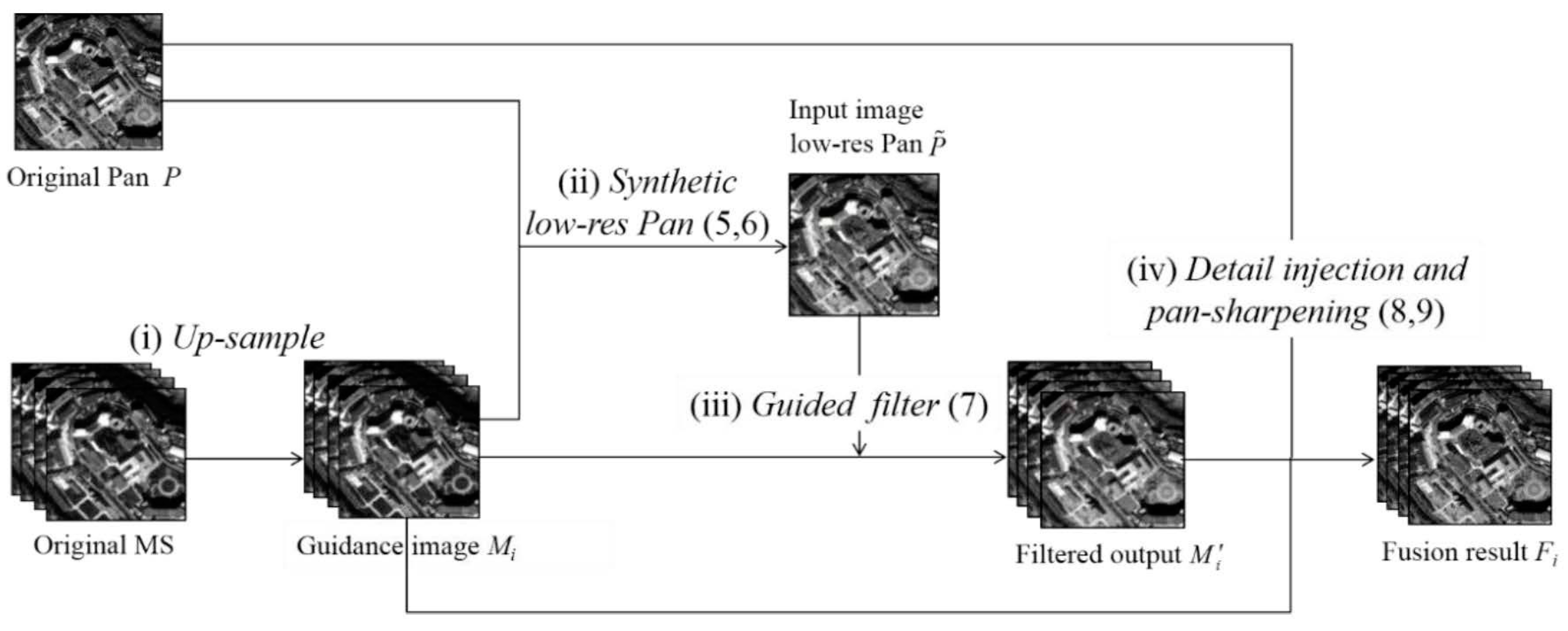
In this section, a pan-sharpening method based on guided image filtering is proposed. The flow chart of the method shown in
Figure 2 can be described as follows.
- (i)
The original multispectral image is registered and resampled to be the same size as the original Pan image .
- (ii)
By minimizing the residual sum of squares (Equation (5)), the weights
(with
) can be easily estimated.
Thereafter, a synthetic low-resolution panchromatic image
can be obtained with Equation (6).
where
is the simulated low-resolution panchromatic image and
is the weight for the
i-th band
, which is constant for the given band.
- (iii)
Each
(with
) is taken as the guidance image to guide the filtering process of the low-resolution Pan image
, and the filter output
(with
) is obtained as follows:
where
denotes the process of guided filtering, and
and
represent the guidance and input images, respectively.
- (iv)
The pan-sharpening result
is obtained by extracting the spatial information from the Pan image and injecting it into the resampled MS image
according to the weight
. This process can be formulated as shown in Equations (8) and (9):
where
is the fusion image,
is the original Pan image,
is the resampled MS image,
is the filtering output,
is the weight corresponding to
i-th MS band at a position
,
denotes a local square window centered at
,
expresses a pixel in the local square window
,
is the band number of the MS image and the total number of bands in the MS image is 4. Obviously, the greater the distance is, the smaller the weight should be; otherwise, the weight should be large.
In the proposed algorithm, the guided filtering involves both the resampled spectral band (as the guidance image) and the simulated Pan band (as the input band); therefore, the output band preserves the structures of both and . This process results in less spectral distortion when extracting the spatial details from the Pan band.
Furthermore, the algorithm modulates the extracted spatial details with a position-dependent ratio . More specifically, as shown in Equation (9), for each pixel located at position centered at a window of size , the Euclidean distance between each and is calculated. Then, the reciprocal of the distance is defined as an indicator of the amount of spatial details that should be injected into a specific MS band. A small distance indicates a small spectrum difference of the corresponding pixels between the MS and Pan bands; in which case, the weight should be large. However, the larger the distance is, the smaller the weight should be; thus, a weak combination is assumed. In this way, the spectral distortion is further reduced.
There are three important parameters in the proposed algorithm: the radius
of local windows, the regularization parameter
in the guided filter, and the radius
of the local windows for calculating the weights. A detailed discussion concerning parameter selections is provided in
Section 5.1.
3.3. Effectiveness of the Proposed Method
The effectiveness of the fused results depends primarily on the detail injection models, that is, the injection weights. A demonstration of detail enhancement and spectral preservation with different weights is provided in
Figure 3 and
Figure 4.
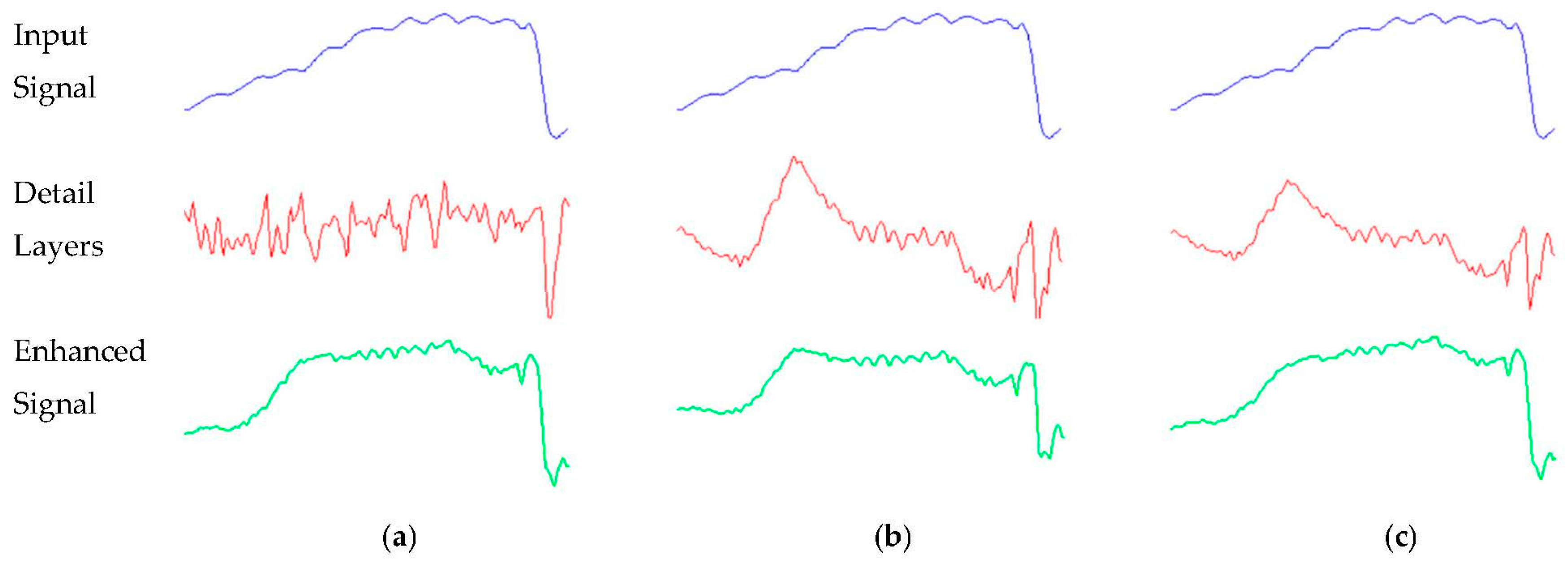
A 1-D example of detail enhancement with different models is shown in
Figure 3. The 1-D input spectral signal (blue) is the spectral curve of part of the features in the first resampled multispectral band
. The product of the
SP (spatial detail) and weight is the injected detail layer (red); among these,
SP expresses the difference between the Pan band and the filtered output. The injection weights include
(Equation (9)), the equal proportion injection model, and the GS-based model [
30] (the covariance between the Pan and first resampled multispectral band). The enhanced signal (green) is the combination of the input signal and the detail layer.
Figure 3a shows that the result obtained from the proposed method with weight
preserves the gradient information well, and the spatial details are obviously simultaneously enhanced. This is because the weight
is calculated pixel-by-pixel, and the spatial details are not lost during processing. However, spatial details are injected in equal proportion in the model; as shown in
Figure 3b, the enhanced signal appears to have an abnormal protrusion. In
Figure 3c, the result based on the GS model has the same trend as the input signal, but the curve is smoother. Due to this global model, some detail may be lost in the fused image.
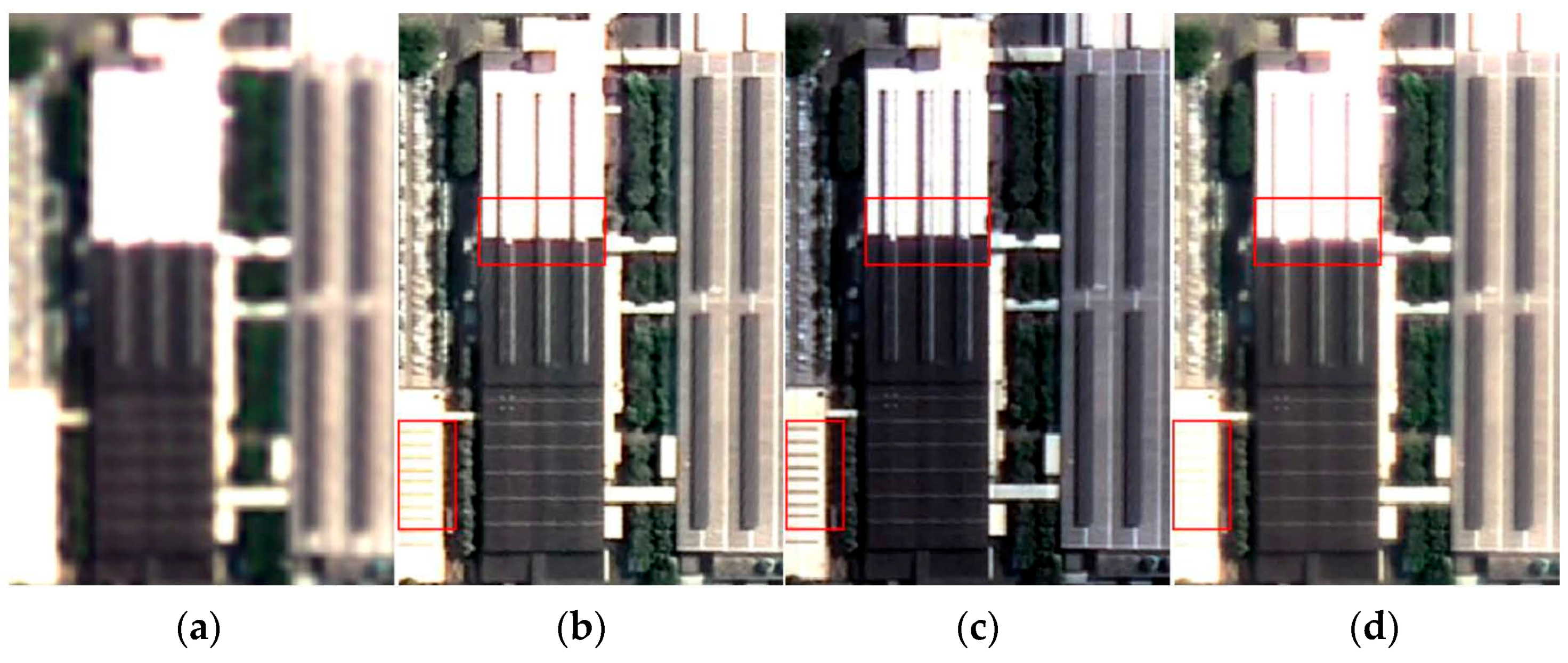
Figure 4 shows a comparison of output images with different injection weights as mentioned above. During processing, the radius and regularization parameter in the guided filter were set to 3 and 10
−8, respectively. The zoomed-in patches indicate that the proposed method, using
as the injection weight, achieves better spectral preservation and detail enhancement than do other models.
5. Results and Discussion
In this section, the influence of the three parameters is discussed first. Successively, four groups of experimental results and some image quality assessment are presented and discussed. Finally, the computational complexity of the proposed method is reported.
5.1. Analysis of the Influence of Parameters
5.1.1. Parameter Influences in the Guided Filter
As mentioned in
Section 2.2, the parameters
and
affect the filtering size and smoothing degree of the guided filter, respectively. To obtain the optimal parameter settings, an image of size 500 × 500 pixels was employed to conduct a parameter analysis, and two metrics, Entropy and SAM, were used as measures. Entropy is related to the spatial quality, while SAM [
33] quantifies the spectral distortion by computing the angle between the corresponding pixels of the pan-sharpened and reference images.
Figure 5 and
Figure 6 show the influences of these two parameters on the pan-sharpening performance.
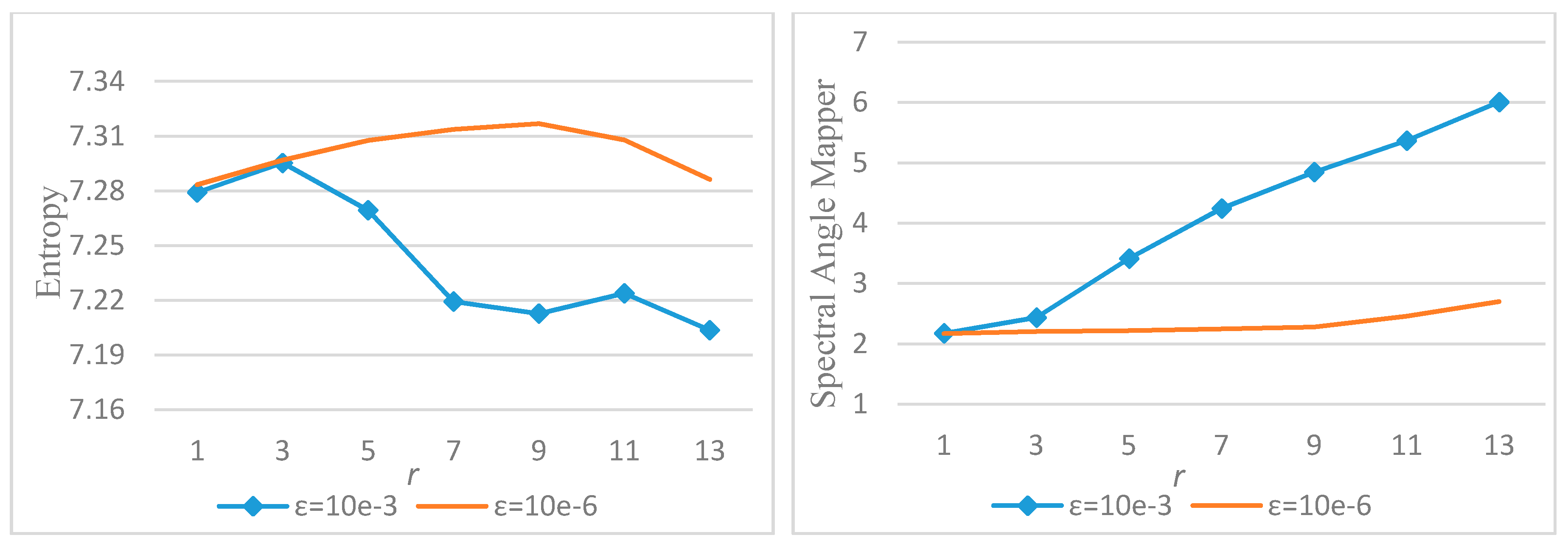
In these experiments, the window size of the weight was fixed to , and 7 groups of both and values were evaluated. When the influence of was analyzed, was fixed to 10−3 and 10−6, while was fixed to 2 and 4 when the influence of was analyzed.
From
Figure 5 we can see that when
is fixed, a larger
reduces the Entropy value and increase the SAM value. However, when
is less than 3, the changes in the Entropy and SAM values are not obvious; and when
is greater than 3, the Entropy value gradually decreases. Therefore, considering the trade-off between the two metrics, the value of
should not be too large or too small.
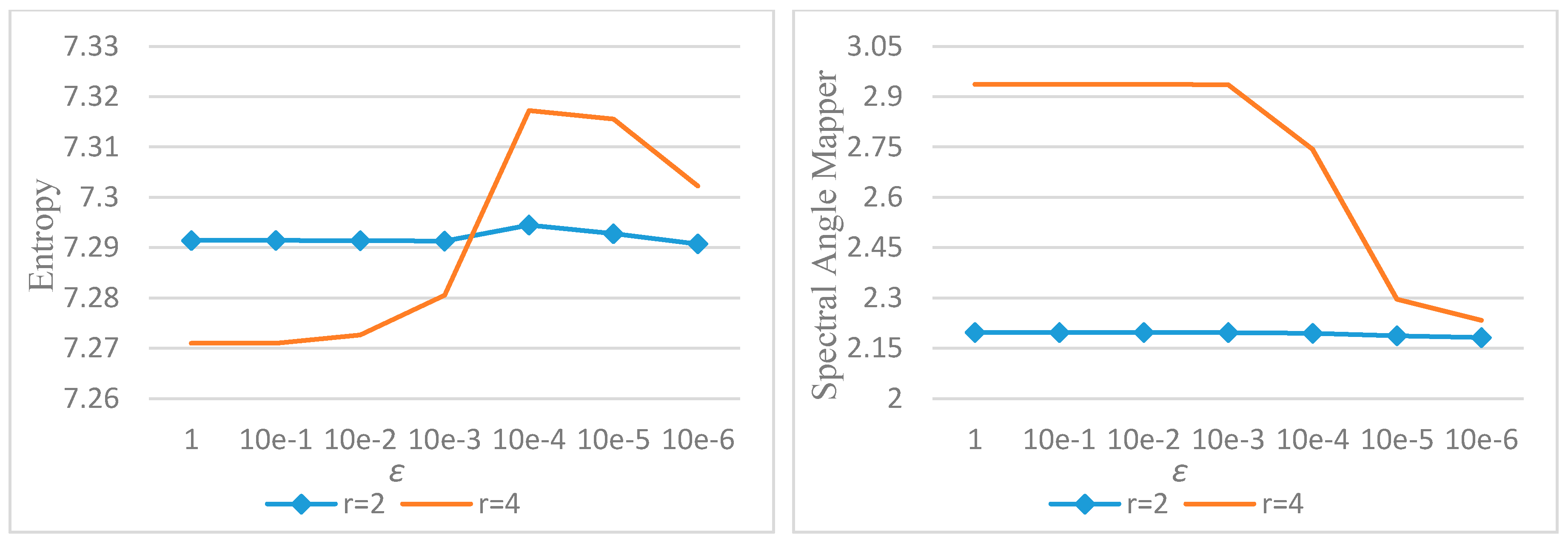
In
Figure 6, when
is fixed, as the
value decreases, the Entropy value becomes larger, while the SAM value continues to decrease. However, an
value greater than 10
−3 has a negligible effect on the Entropy and SAM values, an
value less than 10
−4 causes the Entropy value to decrease slowly, whereas the SAM value decreases continuously. Therefore, the value of
also should not be too large or too small. Consequently, in the following experiments, we set the values of
and
to 3 and 10
−8, respectively.
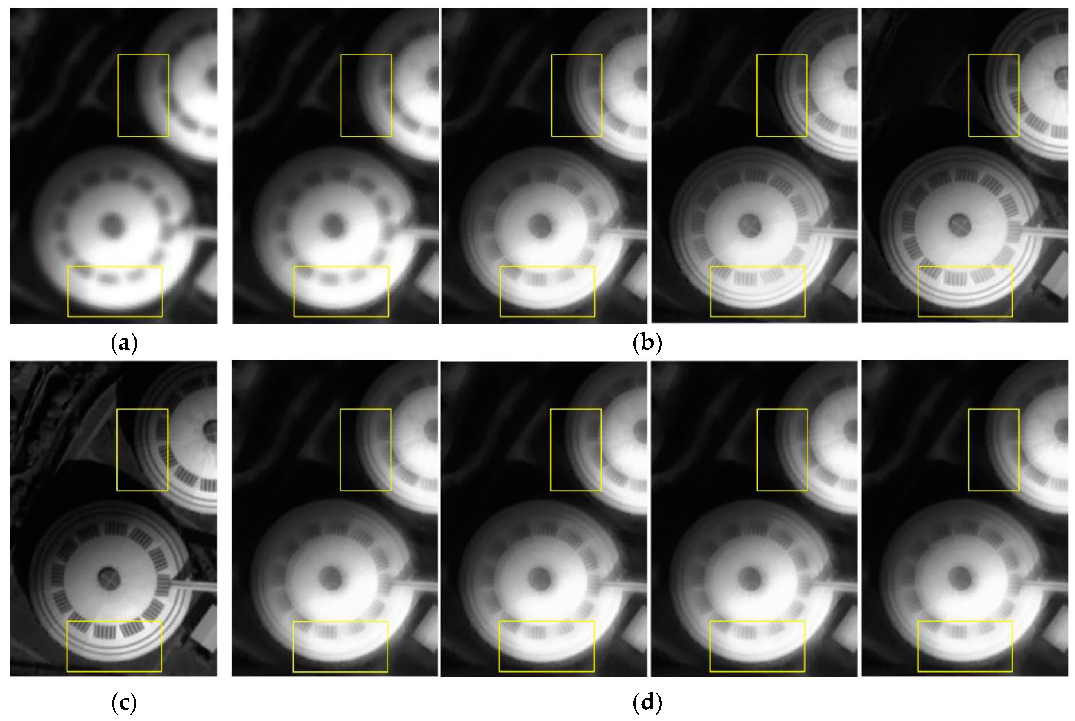
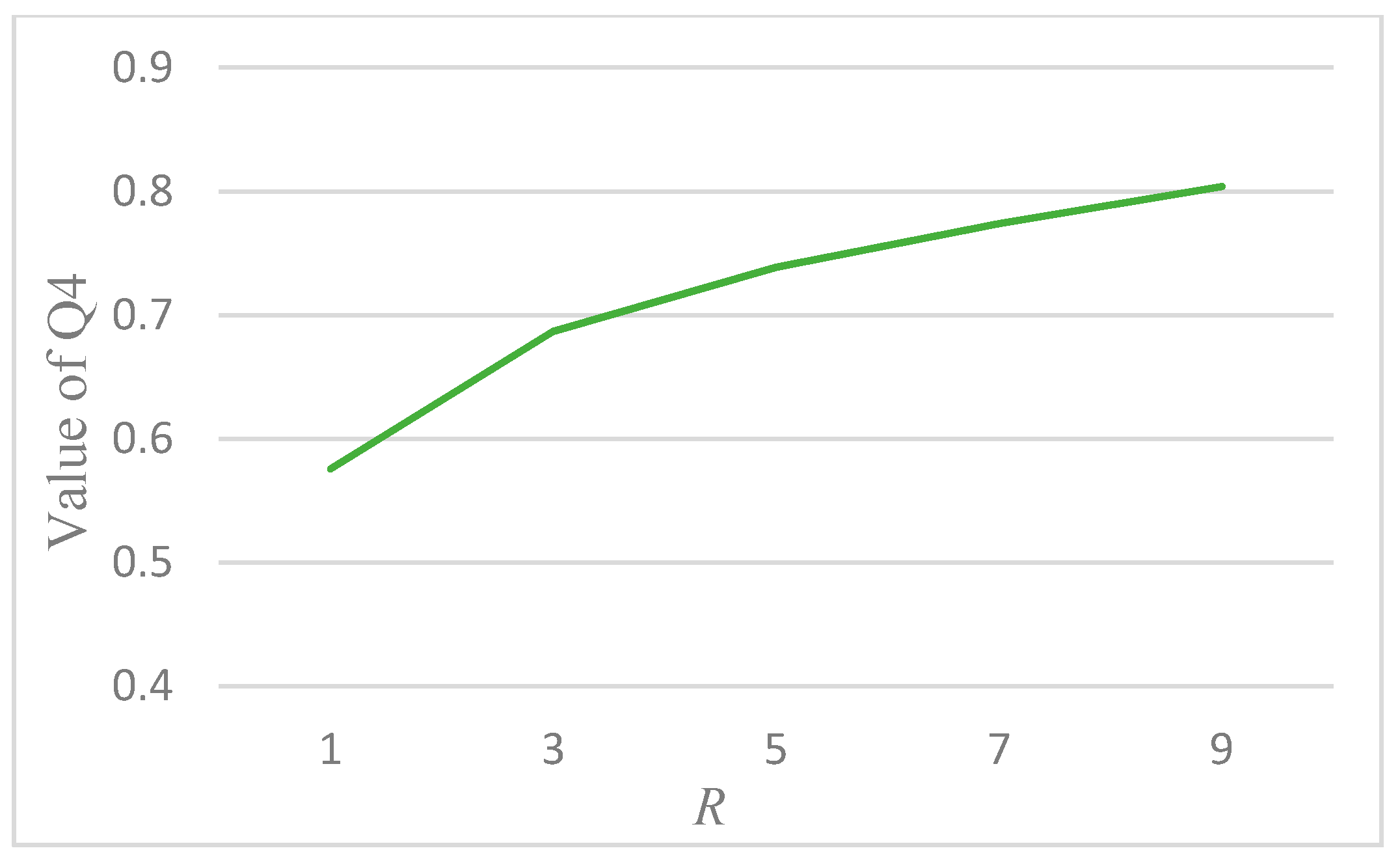
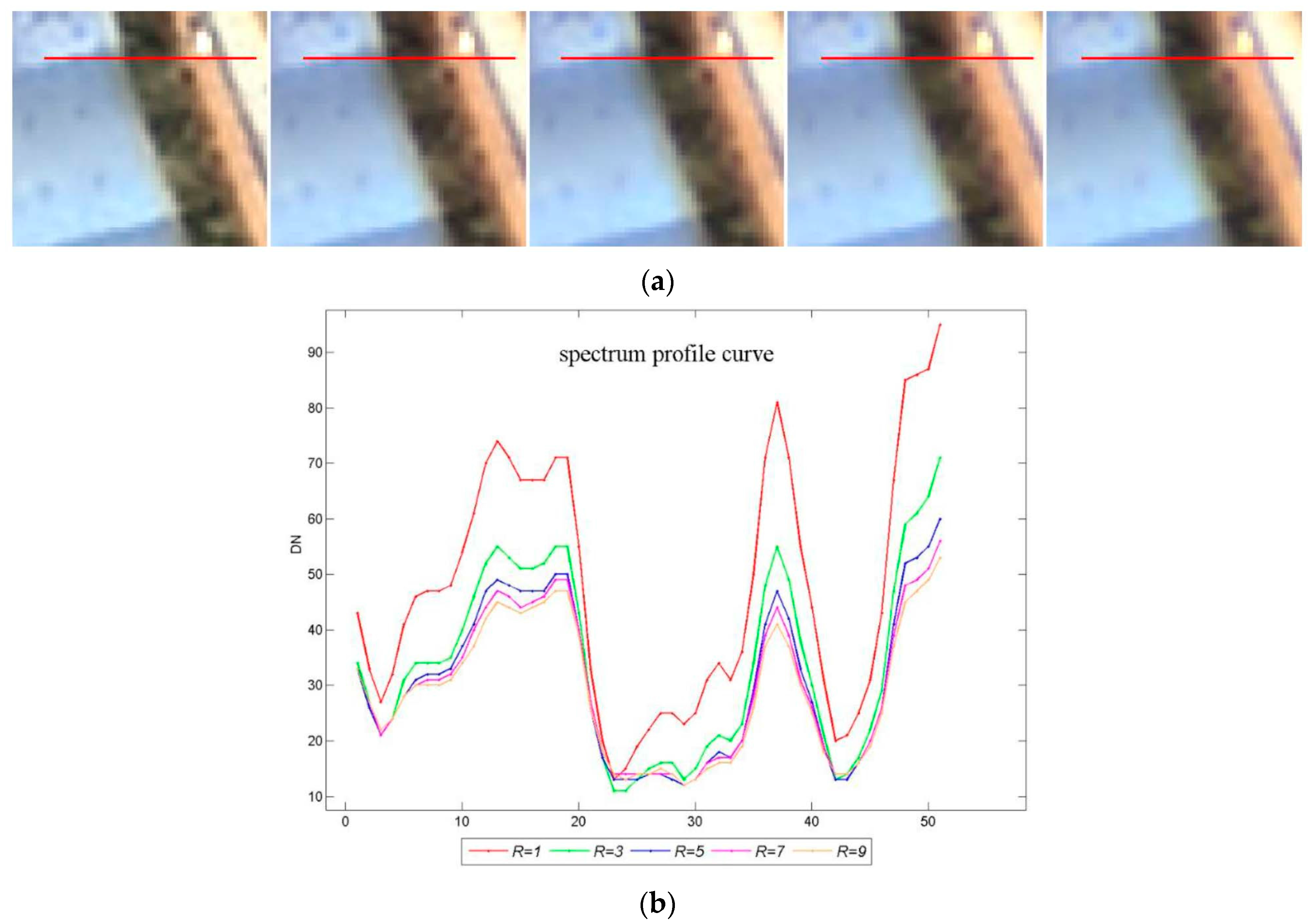
5.1.2. The Influence of the Window Radius for Calculating Weights
The window radius
of the weight during the fusion process is another important parameter. Here, the values of
and
were fixed at 3 and 10
−8, and
was set to 1, 3, 5, 7, and 9 to analyze its influence on the pan-sharpening performance. A quality index Q4 [
34] was employed as the measure of influence. Q4 was averaged over the whole image to produce a global evaluation index, and all calculations were based on
blocks. The value of Q4 ranges from 0 to 1, and lower values reflect the amount of spectral distortion in the fused product, while high values may indicate that a result is closer to the reference image. In the experiments, the value of
was set to 32.
As shown in
Figure 7, the
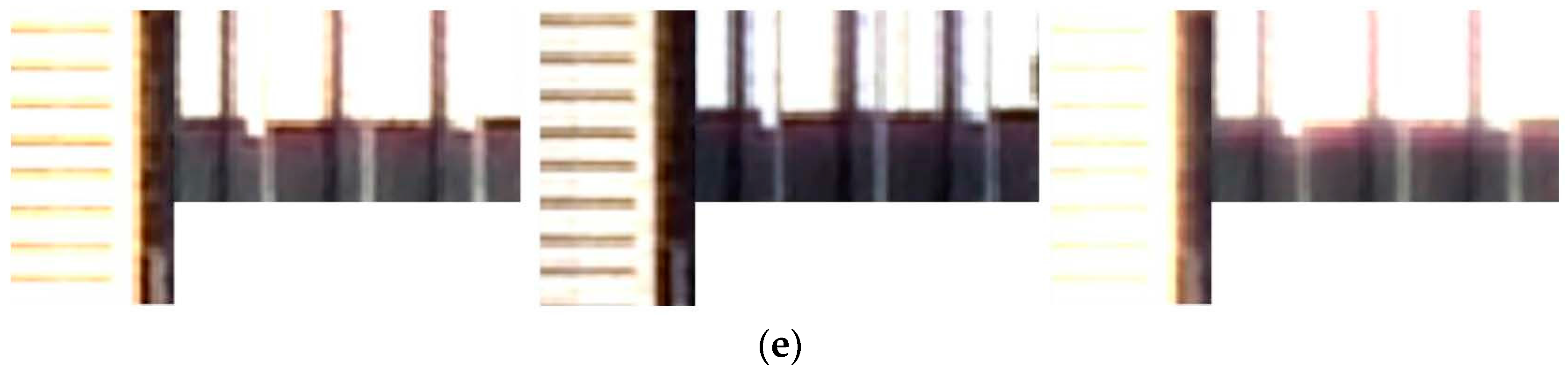
increases, the value of Q4 tends to rise, thus the fusion result had better spectral preservation. However, in some of the detailed pictures of the edge of the building displayed in
Figure 8a, the greater the radius is, the more the spatial details are blurred. Meanwhile, the spectral profile curves of these detailed pictures in the same position are shown in
Figure 8b. As shown, the smaller the
value, the sharper the edges of the corresponding curves become. Therefore, to achieve a better overall effect, the radius
of the weight should not be too small or too large. Considering this trade-off,
was consistently set to 3 in the experiments, that is, the window size for weight calculation was
.
In the above experiments, we found that, according to different metrics (i.e., Entropy, SAM, and Q4), the optimal window sizes for the filtering and weight calculations were consistently set to . Therefore, it is reasonable to set the two window sizes as the same, as both are related to modeling the connections between the Pan and MS bands. Therefore, we assume that the two window sizes are the same.
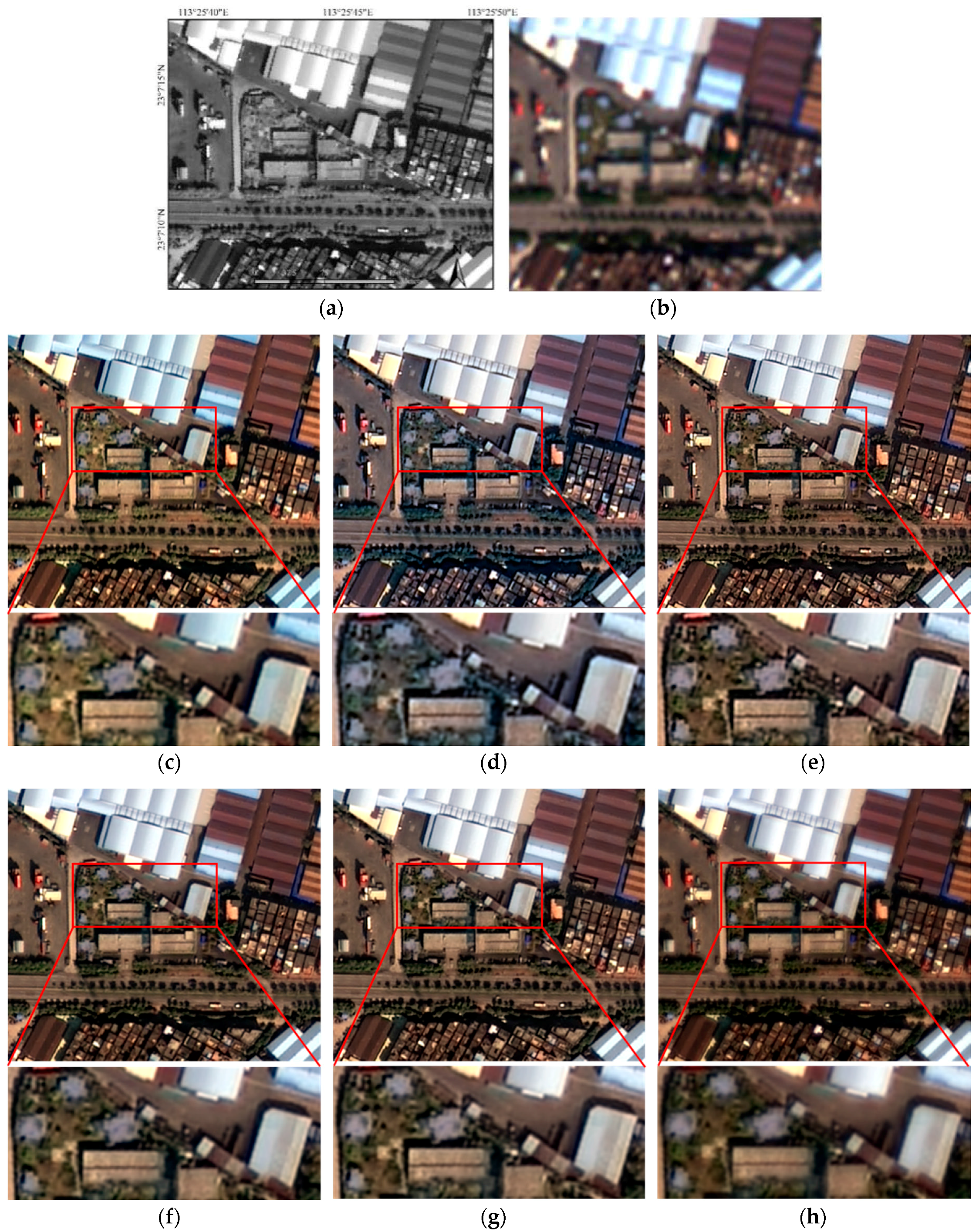
5.2. Comparison of Different Pan-Sharpening Approaches
In this subsection, the proposed pan-sharpening method was compared with some other state-of-the-art approaches. Detailed information about these methods is provided in
Section 4.2. As shown in
Figure 9,
Figure 10,
Figure 11 and
Figure 12, local patches with various land cover types were clipped from the fused results and displayed in true color using the same stretching mode. Quantitative assessments of these four sets of test data are shown in
Table 2,
Table 3,
Table 4 and
Table 5. The best performance of each metric is in bold.
In general, all of the methods yield visually better images than the original. For the urban area (
Figure 9 and
Table 2), the NND method exhibits obvious spectral distortion, and the ERGAS value of the NND method is the largest. From the local detail images, however, the differences between the GS, GSA, UNB, and GD methods are not obvious. Furthermore,
Table 2 shows that the proposed method achieves better spectral and spatial performance; its values for all four metrics are the best.
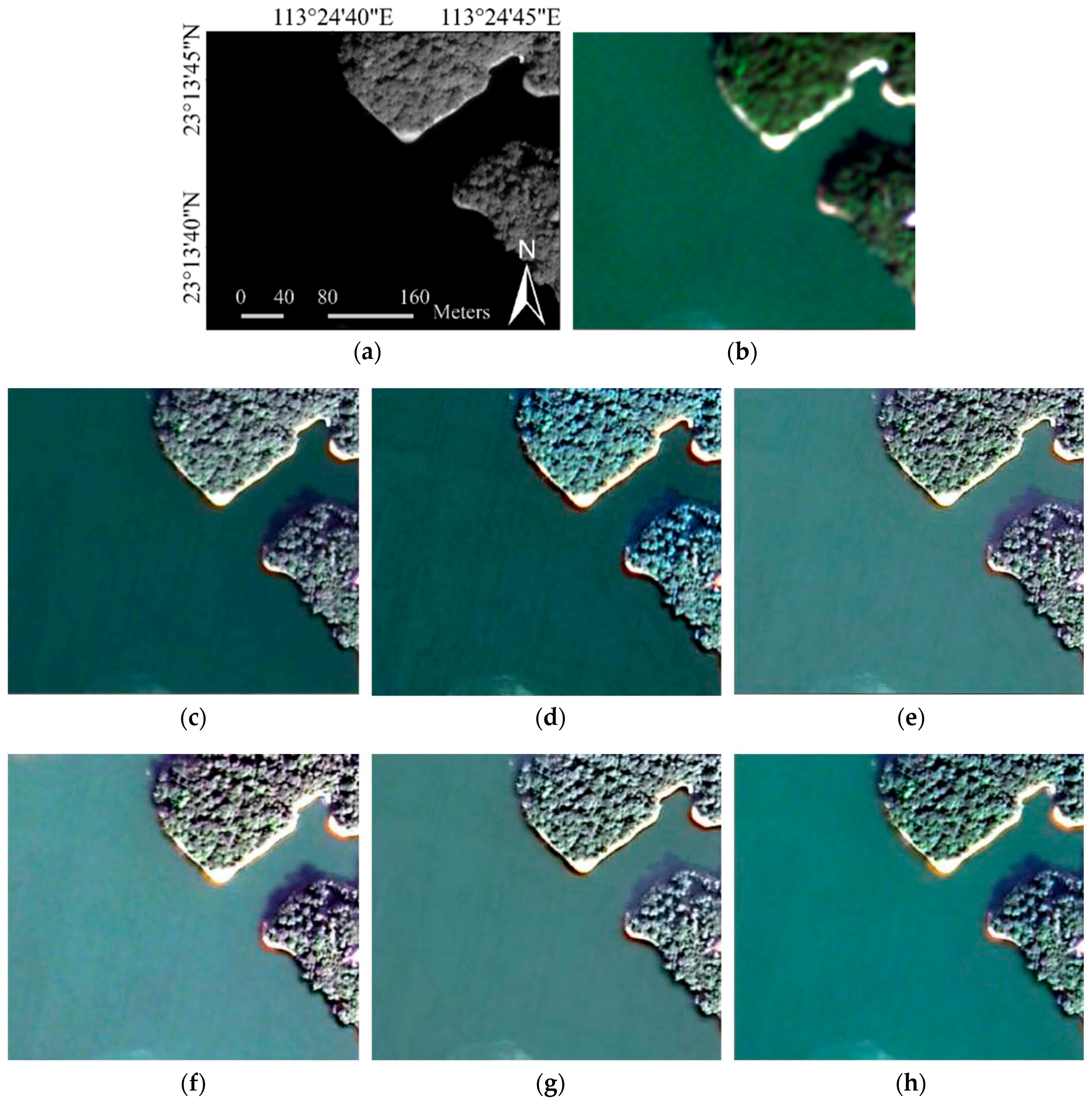
As shown in
Figure 10, the GSA, UNB, and GD methods cannot preserve the spectral information well for water bodies, and the color of the river is paler and not as deep blue as in the original MS image. In
Table 3, we can see that the Entropy value of the NND method is the best; however, its values on the other metrics are the worst. This demonstrates that the NND method performs well in enhancing detail but does not perform well on spectral preservation; this result may have occurred because the NND method is more suitable for fusing low-resolution images.
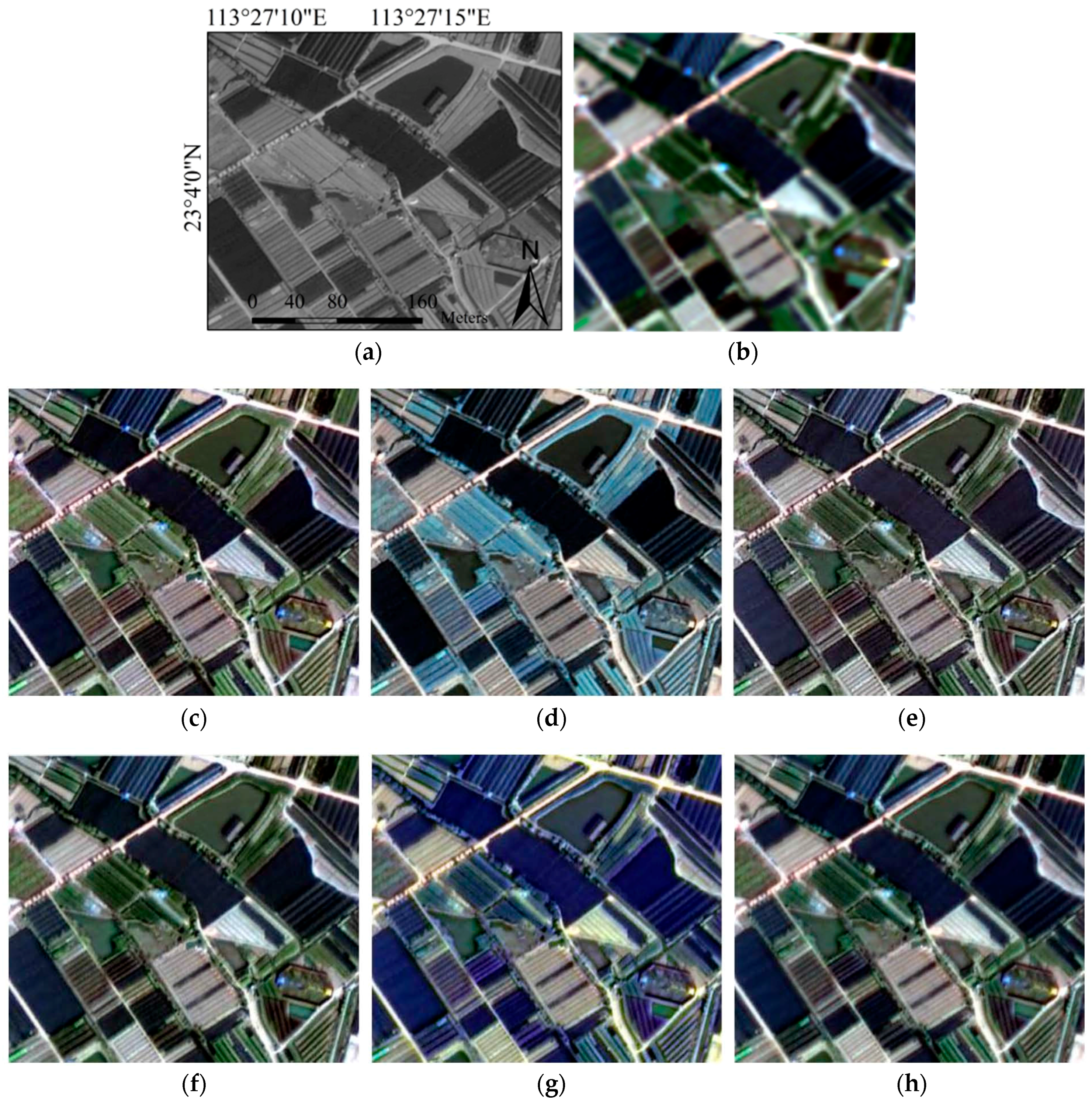
As seen from
Figure 11, the fused images obtained by the NND and GD methods had serious problems with spectral performance: the color of the cropland in their results is obviously quite different from that of the original MS image. In addition, in
Table 4, the NND and GD methods’ UIQI, CC and ERGAS values were the worst, but the overall spatial information was well preserved from a qualitative point of view. This is because the GD method employs a global detail-injection model; thus, color distortion will occur in some specific scenes. However, the proposed method based on the local injection model can be a good solution to spectral distortion. The GS, GSA, and proposed method performed better than the others.
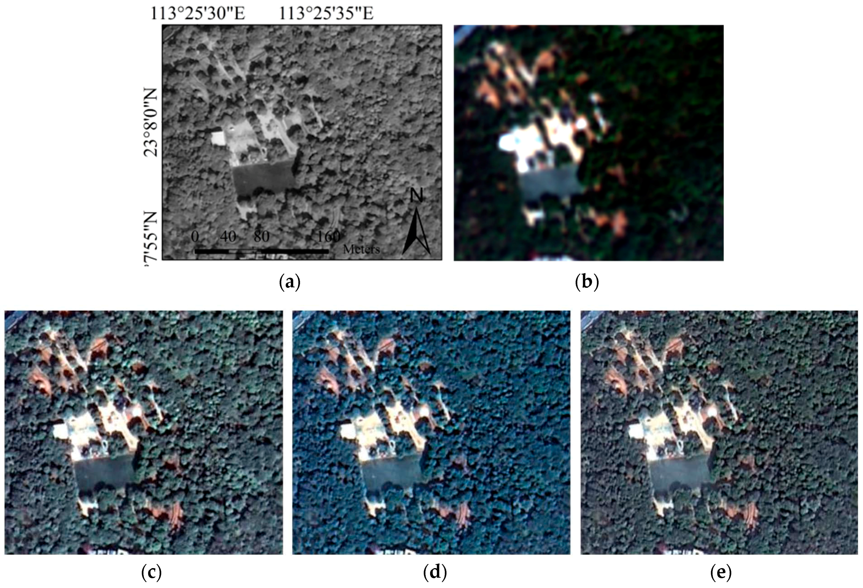
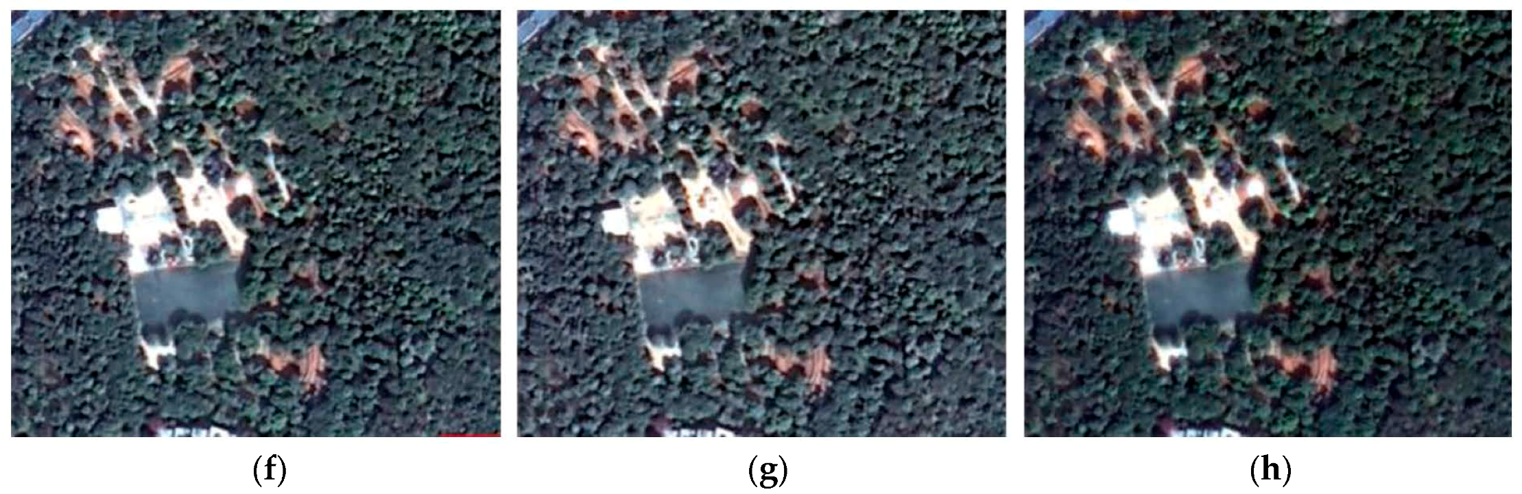
For the forest area shown in
Figure 12 and
Table 5, from a visual analysis, the proposed method achieves the best spectral and spatial information performance compared to the other methods, followed by the GSA, UNB, GS, and GD methods and finally, the NND method. In the quantitative evaluation, the UIQI and CC values of the proposed method were the best, and its ERGAS value was second best, which is consistent with the visual analysis results.
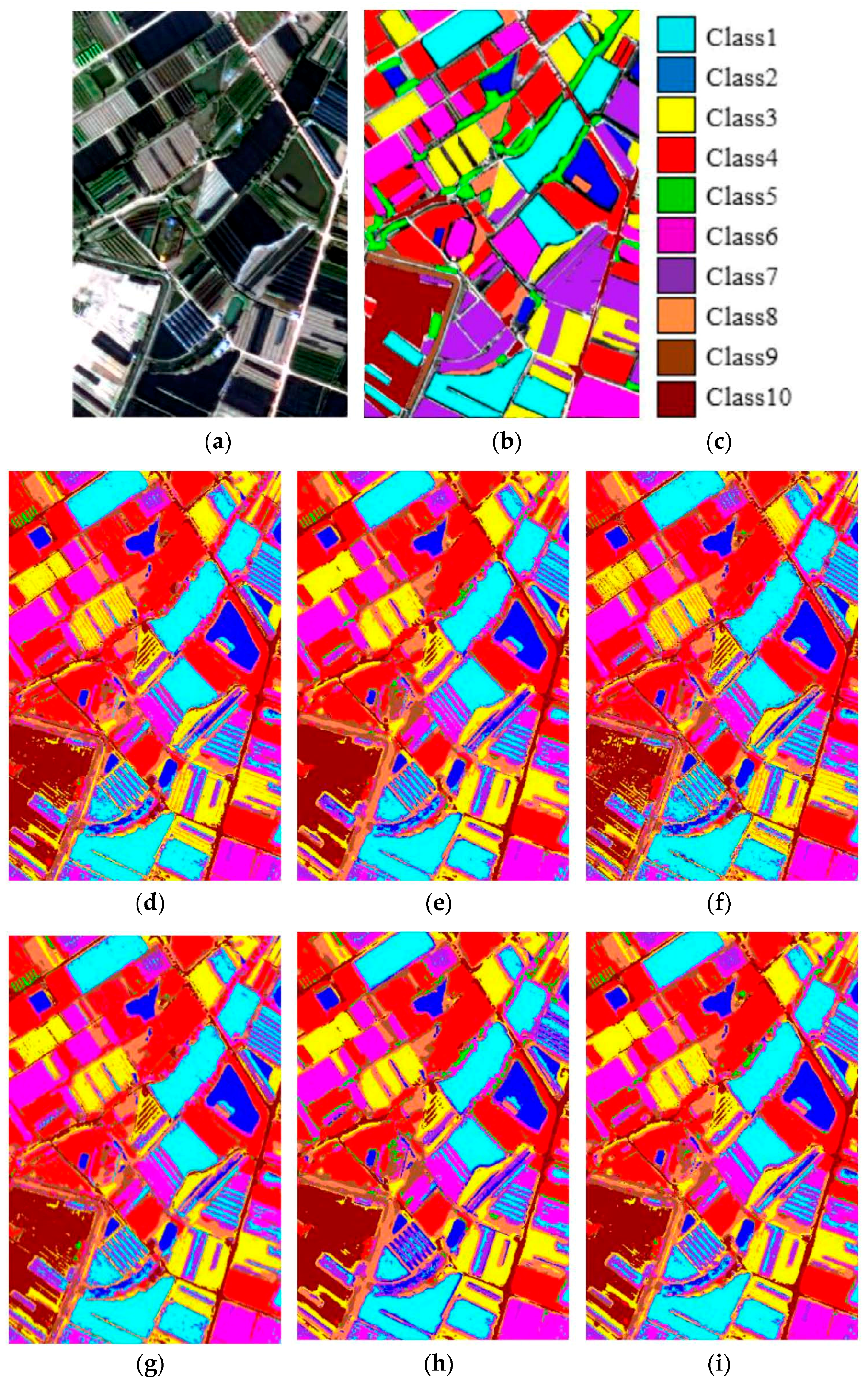
Many pan-sharpened images are employed not only for manual interpretation, but also for computer-based interpretation. Therefore, classification accuracy was used as an indirect evaluation method to verify the effectiveness of the proposed method. A better fusion method should result in fused images with higher interclass variance and, thus, should obtain better classification results. Therefore, in our work, the pan-sharpened images are classified based on spectral features. The overall accuracy (OA) and Kappa are employed as the measures of classification accuracy. The higher the OA and Kappa values are, the better the classification effect is.
In detail, a sample image with a 400 × 600 pixels size was employed to conduct the pan-sharpening process using different methods; then, a supervised classification using a Support Vector Machine (SVM) method [
38] was applied to the fused results.
Figure 13 shows the classification maps, among which,
Figure 13b,c shows the test sample with 157 blocks, including 10 classes. The number of each class in the test sample was 1/10 of the number in the training samples. As can be seen in
Figure 13, the classification results obtained by the NND and UNB methods are not particularly satisfactory. However, the proposed fusion method achieves a more consistent classification result.
Table 6 shows the OA and Kappa precisions achieved by these different methods, corresponding to the classification maps. Although many types of misclassifications occurred, the proposed method achieved the highest accuracy, which means that the proposed method is more effective at spectral preservation than other tested methods.
In conclusion, these experimental results are sufficient to demonstrate that the proposed approach both enhances the spatial information and effectively preserves the spectral characteristics of the original MS images with less distortion. In addition, the produced images can improve the classification accuracy, which is important.
5.3. Computational Complexity
In this section, the computational time of each pan-sharpening method is described to evaluate the computational efficiency. We employed MATLAB on a laptop with 4 GB of memory and a 2.4 GHz CPU to perform the experiments. For a 500 × 500-pixel image, the proposed method requires 11.28 s, while the GS, NND, UNB, GSA, and GD methods require 1.84 s, 1.67 s, 1.52 s, 1.43 s, and 2.36 s, respectively. Compared to the other algorithms, the proposed approach consumes more time; this may be because the weight calculation during the pan-sharpening process is performed in a pixel-by-pixel fashion, and the loop is not efficient enough. Therefore, the speed of the proposed algorithm can be further improved by using a more efficient computational approach.


