2. Preliminaries and Definitions
We denote the set of real numbers by and the two-dimensional real space by . The space containing moving 2-dimensional objects will be denoted . We will use x and y (with or without subscripts) to denote spatial variables and t (with or without subscripts) to denote time variables. The letter T (with or without subscripts) will be used to refer to triangles, which we assume to be represented by triples of pairs of points in .
In this section, we first give the definition of a spatial, a temporal and a spatio-temporal object. Next, we come back to the need of a normal form. Finally, we define affine triangulations of spatial and of spatio-temporal data.
2.1. Spatio-Temporal Data in the Geometric Data Model
In this section, we describe the geometric data model as introduced by Chomicki and Revesz [
1], in which spatio-temporal data are modeled by geometric objects that in turn are finite collections of atomic (geometric) objects. First, we define temporal, spatial and spatio-temporal data objects. In this definition we work with semi-algebraic sets because these are infinite sets that allow a effective finite description by means of polynomial equalities and inequalities. More formally, a semi-algebraic set in
is a Boolean combination of sets of the form
, where
p is a polynomial with integer coefficients in the real variables
,
, ...,
. Properties of semi-algebraic sets are well known [
28].
Definition 1. A temporal object is a semi-algebraic subset of , a spatial object is a semi-algebraic subset of and a spatio-temporal object is a semi-algebraic subset of . ☐
With the
time domain of a spatio-temporal object, we mean its projection on the time axis, i.e., on the third coordinate of
. It is a well-known property of semi-algebraic sets, that this projection is a semi-algebraic set and can therefore be considered a temporal object [
28].
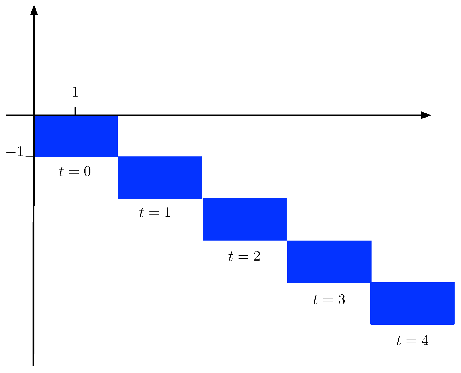
Example 1. The interval and the finite set are examples of temporal objects. The unit circle in the plane is a spatial object, since it can be represented by the polynomial inequalities , usually abbreviated by the formula . The set is a spatio-temporal object and it represents rectangle that is translated at constant speed during the time interval . At each moment t in this interval it has corner points , , and , as illustrated in Figure 1. In
the geometric data model [
1,
4], spatio-temporal objects are finitely represented by geometric objects, which in turn are finite collections of atomic geometric objects. An atomic geometric object is given by its spatial reference object, which determines its shape; a time interval, which specifies its lifespan; and a transformation function, which determines the movement of the object during the time interval.
Several classes of geometric objects were introduced, depending on the types of spatial reference objects and transformations [
1,
4]. In this article, we consider
spatio-temporal objects that can be represented as finite unions of triangles moved by time-dependent affine transformations. We refer also to Definition 2. Other combinations have been studied [
4] in which triangles, rectangles or polygons are transformed by time-dependent translations, scalings or affinities, that, in turn, are given by linear, polynomial or rational functions of time. The class of geometric objects that we consider is not only the most general of the classes that were previously studied, it is also one of the few classes that have the desirable property of being closed under the set operations union, intersection and difference [
4]. In
Section 4, we will rely on this closure property.
Definition 2. An atomic geometric object is a triple , where
is the spatial reference object of , which is a (filled) triangle with corner points that have rational or algebraic coefficients. For technical reasons, we allow a triangle to degenerate into a line segment or a point;
is the time domain (a point or an interval) of ; and
is the transformation function of , which is a time-dependent affinity of the form
where and are rational functions of t (i.e., of the form , with and polynomials in the variable t with rational coefficients) and the determinant of the matrix of the ’s differs from zero for all t in I. ☐
We remark that this definition guarantees that there is a finite representation of atomic geometric objects by means of the polynomial constraint description of the time-interval, (the cornerpoints of) the reference triangle and the coefficients of the transformation matrices. An atomic geometric object
finitely represents the spatio-temporal object
which we denote as
. Atomic geometric objects can be combined to more complex geometric objects.
Definition 3. A geometric object is a set of atomic geometric objects. It represents the spatio-temporal object ☐
By definition 3, the atomic geometric objects that compose a geometric object are allowed to overlap in time as well in space. This is a natural definition, but we will see in
Section 2.2, that this flexibility in design leads to expensive computations when we want to query spatio-temporal objects represented this way.
We define the time domain of a geometric object to be the smallest time interval that contains all the time intervals of the atomic geometric objects (this is the convex closure of these time intervals, denoted by ).
Remark that a spatio-temporal object is empty outside the time domain of the geometric object that defines it. Also, within the time domain, a spatio-temporal object is empty at any moment when no atomic object exists.
Example 2. The spatio-temporal object of Example 1 can be represented by the geometric object , where is represented by (, , f) and equals (, , f), with the triangle with corner points , , , the triangle with corner points , , , and f the transformation ↦
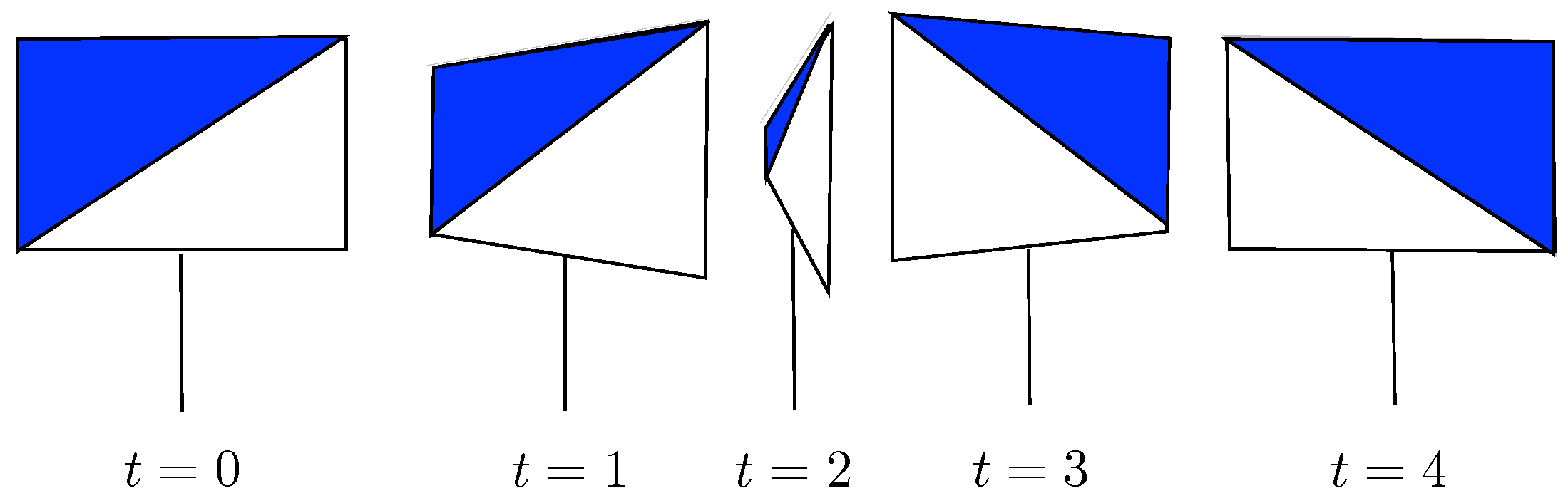
Example 3. Figure 2 shows a traffic sign at six moments (seen by an observer walking around it). This observation can be described by seven atomic geometric objects. During the interval , there exist three atomic objects, two triangles, and one line segment. At the time instant there exists one atomic object that represents the shape of a line. During the interval , there exist three atomic objects, two triangles, and a line segment. To end this subsection, we define the snapshot of a spatio-temporal object at a certain moment in time. Snapshots are spatial objects that show what a spatio-temporal object looks like at a certain moment.
Definition 4. Let be an atomic object. Let be a time moment in the time domain of . The snapshot of at time , denoted , is the intersection of the spatio-temporal object with the plane in defined by , i.e., the plane .
Let be a geometric object. The snapshot of at time , denoted , is the union of the snapshots at of all atomic objects that compose , i.e., . ☐
As explained in Example 3,
Figure 2 shows six snapshots of a geometric object representing a traffic sign seen by a moving observer.
2.2. The Benefits of a Normal Form
As remarked after Definition 3, the atomic objects that compose a geometric object may overlap both in space as in time. As a consequence, it is impossible to answer some very basic queries about a geometric object without a lot of computations.
To know the time domain of a spatio-temporal object, for example, one needs to check all atomic objects that describe it, sort the begin and end points of their time domains, and derive the union of all time domains.
Also, there might be atomic objects that do not contribute at all to the shape of the spatio-temporal object as they are entirely overlapped by other atomic objects. These objects are taken along unnecessarily in computations. Furthermore, two geometric objects that represent the same spatio-temporal object can have a totally different representation by means of atomic objects. It is computationally expensive to derive from their different representations that they are actually the same.
These drawbacks can be solved by introducing a normal form for geometric objects, that makes their structure more transparent. This normal form should have the property that it is the same for all geometric objects that represent the same spatio-temporal object, independent of their initial representation by means of atomic objects. In this paper, we add the requirement that this normal form should be invariant under affinities. If two geometric objects are the same up to time-dependent affinities, we also want their normal form representation to be the same up to these affinities.
2.3. Affine Triangulation Methods
We end this section with the definition of affine spatial and spatio-temporal triangulation methods. We remark that, in the following definition, we consider filled triangles and we allow a triangle to degenerate into a closed line segment or a point.
We use the notion of the interior of a set as follows: the interior of a triangle is its topological interior; the interior of a line segment is the segment without endpoints; and the interior of a point is the point itself.
Definition 5 (Spatial and spatio-temporal triangulation). Let be a geometric object and be a time moment in the time domain of {}.
A collection of triangles in is a triangulation of the snapshot if the interiors of different are disjoint and the union equals .
A geometric object is a triangulation of a geometric object if for each in the time domain of , is a triangulation of the snapshot and if furthermore . ☐
We remark that in the second part of Definition 5, at each moment in the time domain of , may be empty (i.e., may be outside the time domain of ).
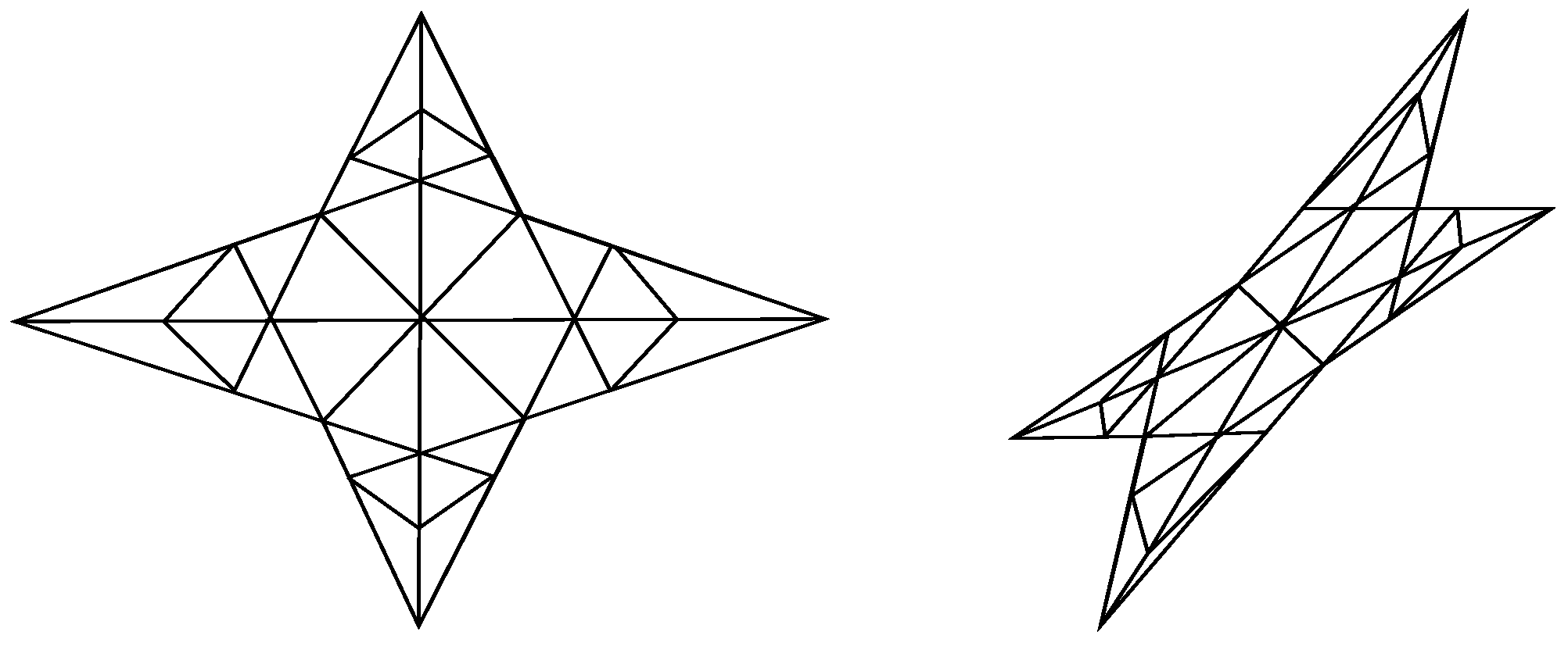
In
Figure 3, two stars with their respective triangulations are shown. Note that, although triangulations of spatial sets intuitively are
partitions of such sets into triangles, they are not partitions in the mathematical sense. Indeed, the elements of the
partition may have common boundaries. For spatial data, it is customary to allow the elements of a partition to share boundaries (see for example [
11]).
A spatial triangulation method is a procedure that on input (some representation of) a snapshot of a spatio-temporal object produces (some representation of) a triangulation of this snapshot. A spatio-temporal triangulation method is a procedure that on input (some representation by means of geometric objects of) a spatio-temporal object, produces (some representation by means of geometric objects of) a triangulation of this spatio-temporal object.
Next, we define what it means for such methods to be affine-invariant.
Definition 6 (Affine-invariant triangulation methods). A spatial triangulation method is called affine invariant if and only if for any two snapshots A and B, for which there is an affinity such that , also .
A spatio-temporal triangulation method is called affine invariant if and only if for any geometric objects and for which for each moment in their time domains, there is an affinity such that if also ☐
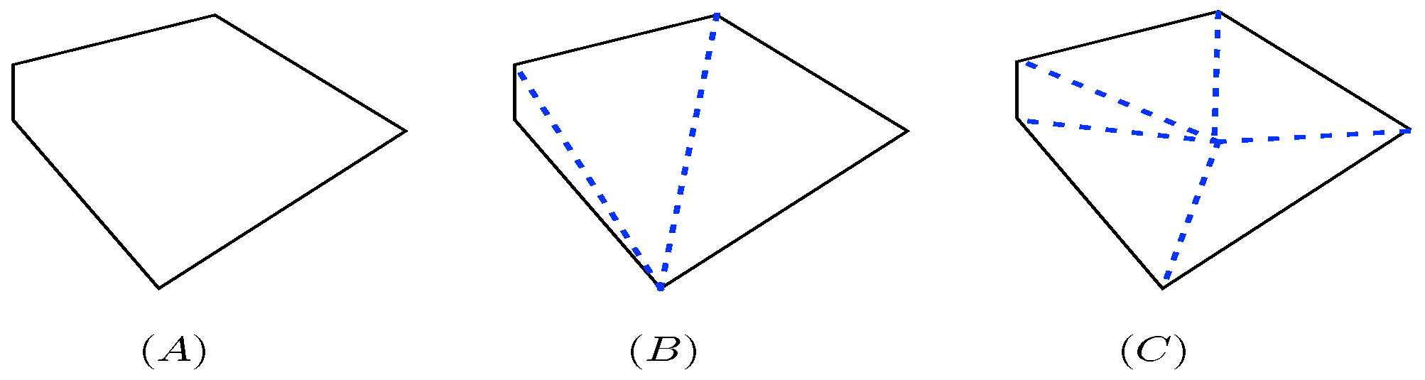
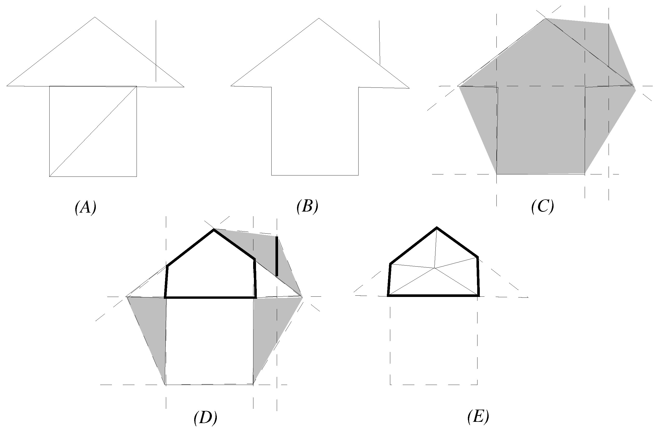
Example 4. Given a convex polygon as shown in of Figure 4. A spatial triangulation method that takes the leftmost of the corner points with the smallest y-coordinates of the polygon and connects it with all other corner points, is not affine invariant. It is not difficult to see that, when an affine transformation is applied to the polygon, another point may become the leftmost lowest corner point. Part of Figure 4 shows the result of applying this triangulation method to the convex polygon shown in . A triangulation method that computes the barycenter of a convex polygon and connects it with all corner points is affine-invariant. An illustration the output of this method applied to the polygon shown in is shown in of Figure 4. We now propose an affine-invariant spatial triangulation method for spatial figures that are snapshots of geometric objects, or, that can be represented as finite sets of triangles.
3. An Affine-Invariant Spatial Triangulation Method
We next propose an affine-invariant triangulation method. Later on, in
Section 4, we will use the technique proposed here to construct a spatio-temporal triangulation algorithm. We first explain the intuition behind the triangulation method, and then give the details in Algorithm 1. We illustrate the algorithm with an example, prove its correctness and end with determining the size of the output and the time complexity of the algorithm.
Intuitively, the algorithm is as follows. The input is a snapshot
S, given as a finite set of triangles. In
Figure 5A, for example, a snapshot of a house-like shape is given by four triangles. One of those triangles is degenerated into a line segment (representing the chimney). To make sure that the triangulation is independent of the exact representation of the snapshot by means of triangles, the boundary of the snapshot, i.e., the boundary of the union of the triangles composing
S, is computed. For the snapshot of
Figure 5, the boundary is shown in (B). The (triangle degenerated into A) line segment contributes to the boundary. Therefor, we label it, the reason for this will become clear in a further stage of the procedure. Also, the (triangles degenerated into) points of the input that are not part of a line segment or real triangle, i.e., the ones contributing to the boundary, are added to the output immediately.
The set of all lines through the edges of the boundary partitions the plane into a set of open convex polygons, open line segments, open (half-) lines and points. The (half-) lines and some of the polygons can be unbounded, so we use the convex hull
of the corner points of all triangles in the input as a bounding box. In (C) of
Figure 5, the grey area is the area inside of the convex hull. The partition of the area inside the convex hull is computed. The points in this partition are not considered. The points contributing to the boundary were already added to the output in an earlier stage. For each open line segments, it is checked whether it is part of a labelled line segment of the input. Recall that only line segments that contribute to the boundary are labelled in an earlier stage of the algorithm. Only if an open line segment is part of a labelled segment, as is the case for the one printed in bold in
Figure 5D, its closure (i.e., a closed line segment) is added to the output. For each open polygon in the partition, we compute the polygon that is its closure and triangulate this polygon using its center of mass (see
Figure 5D for a polygon in the partition and (E) for its triangulation). Some open polygons are only part of the convex hull of
S, but not of the snapshot itself. The polygons shaded in grey in (D) of
Figure 5 are an example of such polygons. If a polygon does not belong to
S, we do not triangulate it. The triangulations of all other polygons are added to the output. Note that we can decide whether a polygon belongs to the snapshot by first computing the
planar subdivision (which we will define next) of the input snapshot and then test for each open polygon whether its center of mass belongs to the interior of a region or face in the subdivision. We will explain this in more detail when analyzing the complexity of the algorithm.
In the detailed description of the algorithm, we will use some well known techniques. One of those is the
doubly-connected edge list [
29], used to store
planar subdivisions.
Definition 7 (Planar subdivision). A planar subdivision is a subdivision of the plane into labelled regions (or faces), edges and vertices, induced by a plane graph. The complexity of a subdivision is the sum of the number of vertices, the number of edges and the number of faces it consists of. ☐
Next, we describe the doubly-connected edge list, a data structure to store planar subdivisions. For this structure, each edge is split into two directed half-edges. In general, a doubly-connected edge list contains a record for each face, edge and vertex of the planar subdivision.
Definition 8 (Doubly-connected edge list). Given a planar subdivision . A doubly-connected edge list for , denoted DCEL(), is a structure containing a record for each face, edge and vertex of the subdivision. These records store the following geometric and topological information:
- (i)
The vertex record of a vertex stores the coordinates of and a pointer to an arbitrary half-edge that has as its origin;
- (ii)
The face record of a face f stores a pointer to an arbitrary half-edge on its boundary. Furthermore, for each hole in f, it stores a pointer to an arbitrary half-edge on its boundary;
- (iii)
The half-edge record of a half-edge e stores five pointers. One to its origin-vertex, one to its twin half-edge, one to the face it bounds, and one to the previous and next half-edge on the boundary on that face.
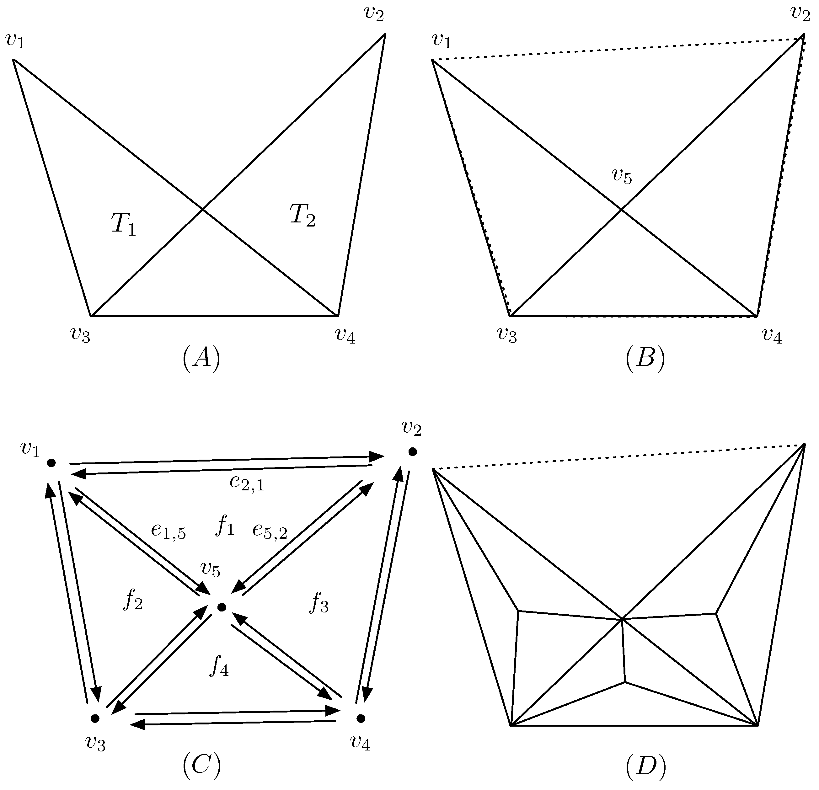
Example 5. Figure 6 shows a planar subdivision in (B) and its topological structure in (C), that is reflected in the doubly-connected edge list represented in Table 2. Algorithm 1 (or ) gives the triangulation procedure more formally. The input of this triangulation algorithm is a snapshot S, consisting of a geometric object which we assume to be given as a finite set of (possibly overlapping and possibly degenerated) triangles. We further assume that each triangle is represented as a triple of pairs of coordinates, which are rational numbers.
To shorten and simplify the exposition of Algorithm 1, we assume that S is fully two-dimensional, or equivalently, that points and line segments that are not adjacent to a polygon belonging to S are already in the output. Including their triangulation in the algorithm would make its description tedious, as we would have to add, and consider, more node and edge labels.
We use C programming-style notation for pointers to records and elements of records. For example, Let . In the vertex record of , and . Let e be an edge record. The coordinates of the origin of e are and .
| Algorithm 1 (Input: S = {, , …, }, Output: {, , …, }) |
- 1:
Out:= ∅. - 2:
Compute the set containing all line segments, bounding a triangle of the input, that contribute to the boundary of S (i.e., that contain an edge of the boundary). Meanwhile, construct the planar subdivision induced by the triangles composing S. - 3:
Compute the convex hull of S. - 4:
Construct the doubly connected edge list DCEL(S), induced by the planar subdivision defined by the lines through the segments of , using as a bounding box. - 5:
while there are any unvisited half-edges in DCEL() left do - 6:
Let e be an unvisited edge. - 7:
, , count := 0, Elist := ∅. - 8:
while e is unvisited do - 9:
Mark e with the label visited. - 10:
Elist Elist , , , count := count . - 11:
. - 12:
end while - 13:
. - 14:
if the point in belongs to a face of then - 15:
for all elements of Elist do - 16:
Out := Out , where is the (closed) triangle with corner points , and . - 17:
end for - 18:
end if - 19:
end while - 20:
return Out.
|
Before proving the correctness of the algorithm and determining the size of the output and the time complexity of the algorithm, we give an example.
Example 6. Let S be the set , where is the triangle with corner points , and , and the triangle with corner points , and , as depicted in Figure 6. The doubly-connected edge list corresponding to is shown in Table 2. We omitted the structures for vertices and faces, as we don’t need them for the second part of the algorithm. After the doubly-connected edge list is constructed, we create and output the triangles. This is done by visiting all half-edges once. Suppose we start with . The next-pointers lead to and . The next pointer of the last one points to , which we visited already. This means we visited all edges of one polygon. The center of mass can now be computed and the triangles added to the output. This is done for all polygons that are part of the input. In this example, the polygon with corner points , and will not be triangulated, as it is not part of the input. The algorithm stops when there are no more unvisited edges left.
Note that, as an optimization, we could decide to not triangulate faces that are triangles already. This does not influence the complexity results, however. Therefor, and also for a shorter and more clear exposition, we formulated the algorithm in a more general form.
We now prove compute the complexity of both the output and execution time of the triangulation method described in Algorithm 1 and afterwards show that it is affine-invariant. First, we show that is indeed a triangulation method.
Property 1 (Algorithm 1 is a triangulation method). Let S be a snapshot. The output of Algorithm 1 applied to S is a triangulation of S.
Proof. Let the set of triangles determine a snapshot S. It is easy to see that the output of is a triangulation. By construction, is a set of triangles that either have no intersection, or share a corner point or bounding segment. It is clear from the algorithm that , because each triangle in is tested for membership of S. We are also sure that S is covered by the output, because initially, the convex hull of S is triangulated, which contains S. ☐
Property 2 (Quadratic output complexity). Let a snapshot S be given by the set , consisting of m triangles. The triangulation , where is the triangulation method described in Algorithm 1, contains triangles.
Proof. It is well-known (see, e.g., [
30]), that an arrangement of
m lines in the plane results in a subdivision of the plane containing
lines,
edges and
faces. It follows that the structure DCEL(
) will contain
half-edges, i.e., two half-edges for each edge in the arrangement. In the worst case scenario, when all faces of the partition of the bounding box belong to
S, one triangle is added to the output for each half-edge in DCEL(
) (connecting that half-edge with the center of mass of the face it bounds). Therefor, the output contains
triangles. ☐
In the following analysis of the running time of Algorithm 1, we assume that triangles are represented as triples of points, and that a point is represented as a pair of rational or algebraic numbers. We further assume that all basic arithmetic operations on coordinates of points require constant time.
Property 3 ( running time). Let a snapshot S be given by the set , consisting of m triangles. The triangulation method , described in Algorithm 1, computes the triangulation of S in time .
Proof. Let a snapshot
S be given by the set
. Using a plane-sweep algorithm [
31], we compute both the list of segments contributing to the boundary of
S and the planar subdivision
induced by
. This takes
, as there are at most
intersection points between boundary segments of triangles of
S.
The
m triangles composing
S together have at most
different corner points. Computing the convex hull of
m points in the plane can be done in time
(see [
32]). The same authors propose, in [
30], an algorithm to compute a doubly-connected edge list, representing an arrangements of
m lines, in time
. We next show that the changes we make to this algorithm do not influence its running time. So, as
contains at most all
line segments, it induces an arrangement of at most
lines. Hence, Step 3 of Algorithm 1 also takes time
.
We changed the original algorithm [
30] for computing the doubly-connected edge list of an arrangement of lines as follows:
- (i)
We computed the convex hull of the input to serve as a bounding box instead of an axis-parallel rectangle containing all intersection points of the arrangement. The complexity of computing such an axis-parallel rectangle is higher () than that of computing the convex hull ().
- (ii)
The cost of constructing the doubly-connected edge list of the convex hull is
, as the convex hull contains at most
corner points and the algorithm for computing it, as described in [
32], already outputs the corner points of the convex hull in circular order. In the original algorithm [
30] with an axis-parallel bounding rectangle, computing the doubly-connected edge list of this rectangle only takes constant time. This extra time does, however, not affect the overall complexity.
- (iii)
The next step of both algorithms involves finding the intersection points between the lines to be inserted and the partial arrangement induced by the previously inserted lines. In the original algorithm, this is easier only for the intersection of a line with the bounding box. For the intersections with all other lines in the arrangement, the cost is the same.
The next part of Algorithm 1 (starting from Line 5) takes time
. Each half-edge of the doubly-connected edge list is visited only once. Also, each half-edge is only inserted once into the set
Elist, and consulted only once therein to create a triangle. As an arrangement of
m lines in the plane results in
edges, the number of half-edges in DCEL(
) also is
. We can, in time
, preprocess
into a structure that allows point location in
time [
33]. Therefor, testing for each of the
centers of mass whether they are part of the input takes
. We can conclude that all parts of Algorithm 1 run in time
. ☐
Table 3 summarizes the computational complexity of the various parts of Algorithm 1.
Property 4 ( is affine-invariant). The triangulation method is affine-invariant.
Proof. According to the definition of affine-invariance of spatial triangulation methods (Definition 6), we have to prove the following. Let A be a snapshot given by the set of triangles and B be a snapshot given by the set of triangles , such that there exists an affinity for which . Then, for each triangle T of , it holds that the triangle is a triangle of .
We prove this by going through the steps of the triangulation procedure . Let A and B be as above.
The convex hull and boundary of spatial figures are both affine-invariant (more specific, the boundary is a topological invariant). Intersection points between lines and the order of intersection points on one line with other lines are affine-invariant (even topological invariant). The subdivision of the convex hull of B induced by the arrangement of lines through the boundary of B is hence the image under of the subdivision of the convex hull of A induced by the arrangement of lines through the boundary of A. The doubly-connected edge list only stores topological information about the arrangement of lines, i.e., which edges are incident to which vertices and faces. Naturally, this information is preserved by affine transformations. The center of mass of a convex polygon is an affine invariant. Finally, the fact that a triangle is inside the boundary of the input and the fact that it is not are both affine-invariant. This completes the proof. ☐
Summarizing this section, we proposed a spatial triangulation method that, given a snapshot consisting of m triangles, returns an affine-invariant triangulation of this snapshot containing triangles, in time .
We remark here that the idea of using carriers of boundary segments to partition figures was also used in an algorithm to decompose semi-linear sets by Dumortier, Gyssens, Vandeurzen and Van Gucht [
34]. Their algorithm is not affine-invariant, however.
In the next section, we will use the affine triangulation for snapshots to construct a triangulation of geometric objects.
4. An Affine-Invariant Spatio-Temporal Triangulation Method
In this section, we present an spatio-temporal triangulation algorithm that takes as input a geometric object, i.e., a finite set of atomic geometric objects. We will adapt the spatial triangulation method , described in Algorithm 1, for time-dependent data.
The proposed spatio-temporal triangulation algorithm will have three main construction steps. First, in the partitioning step, the time domain of the geometric object will be partitioned into a set of points and open time intervals. For each element of this partition, all its snapshots have an isomorphic triangulation, when computed by the method . We refer to Definition 9 below for a formal definition of this isomorphism. Second, in the triangulation step, the spatio-temporal triangulation is computed for each element in the time partition, using the fact that all snapshots have isomorphic triangulations. Third, in the merge step, we merge objects when possible, to obtain a unique (and minimal) triangulation.
We will start this section by defining isomorphic triangulations. Then we explain the different steps of the algorithm for computing a spatio-temporal affine-invariant triangulation of geometric objects separately. We illustrate the algorithm with an example and end with some properties of the triangulation.
Intuitively, two snapshots and are called -isomorphic if the triangles in and have the same (topological) adjacency graph. In particular, if and are equal up to an affinity of , then they are -isomorphic.
Definition 9 (-isomorphic snapshots). Let and be two snapshots of a geometric object. We say that and are -isomorphic, denoted , if there exists a bijective mapping with the following property: A triangle of is incident to the triangles , and (where each is either a triangle of that shares the segment with , a triangle of that shares the segment with , or is ϵ, which means that no triangle shares that boundary segment with ) if and only if, the triangle belongs to and is bounded by , and . Moreover, if is a triangle of , then is a triangle of that shares the line segment with , if is a triangle of , then is a triangle of that shares the line segment with and if equals ϵ, then so does . ☐
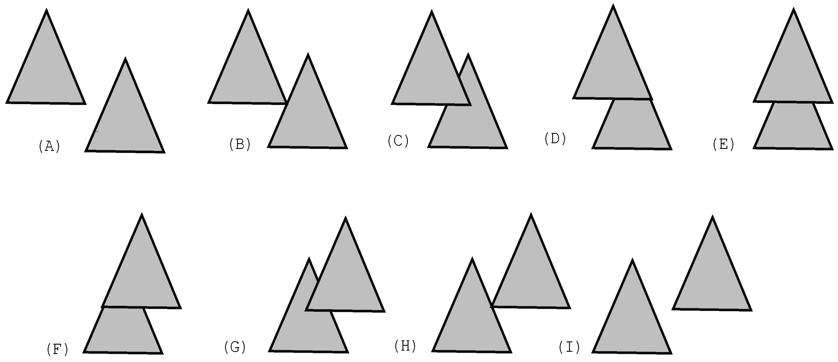
Example 7. The triangulations shown in Figure 3 are -isomorphic to each other. In Figure 7, all snapshots shown except the one at time moment are -isomorphic. The snapshot at time moment is clearly not isomorphic to the others, since it consists only of one line segment. Remark that for
Figure 3, the mapping
h is an affinity. In
Figure 7, this is not the case.
Now, we introduce a spatio-temporal triangulation method that constructs a time-dependent affine triangulation of spatio-temporal objects that are represented by geometric objects. We will explain its three main steps, i.e., the partitioning step, the triangulation step and the merge step separately in the next subsections.
We will illustrate each step on the following example.
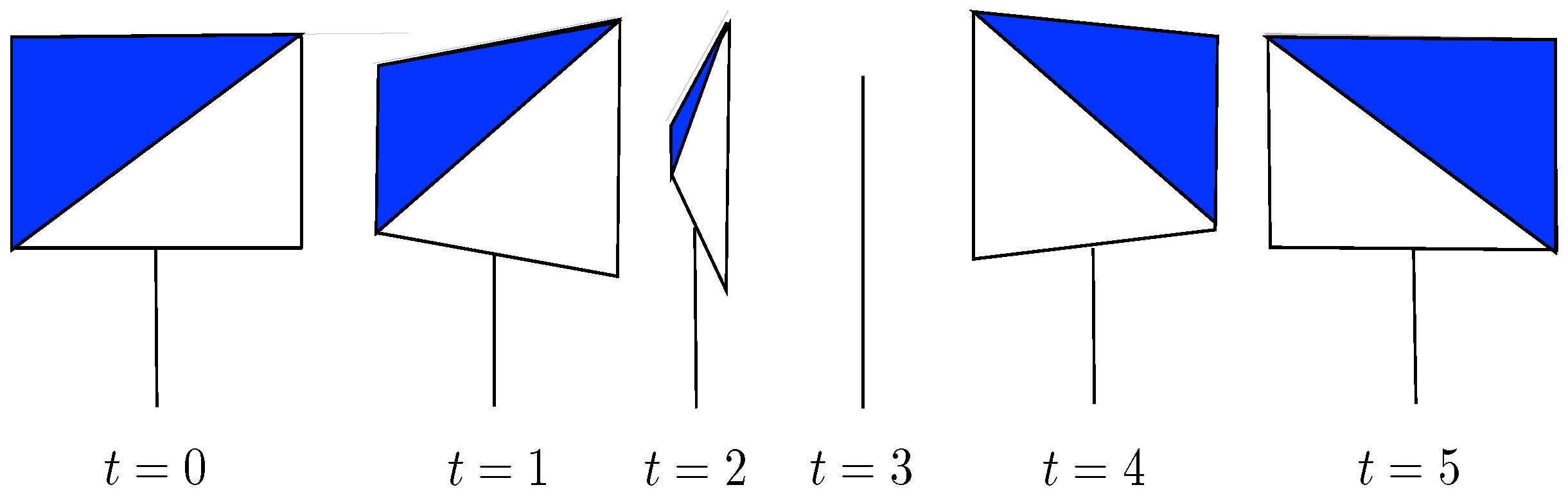
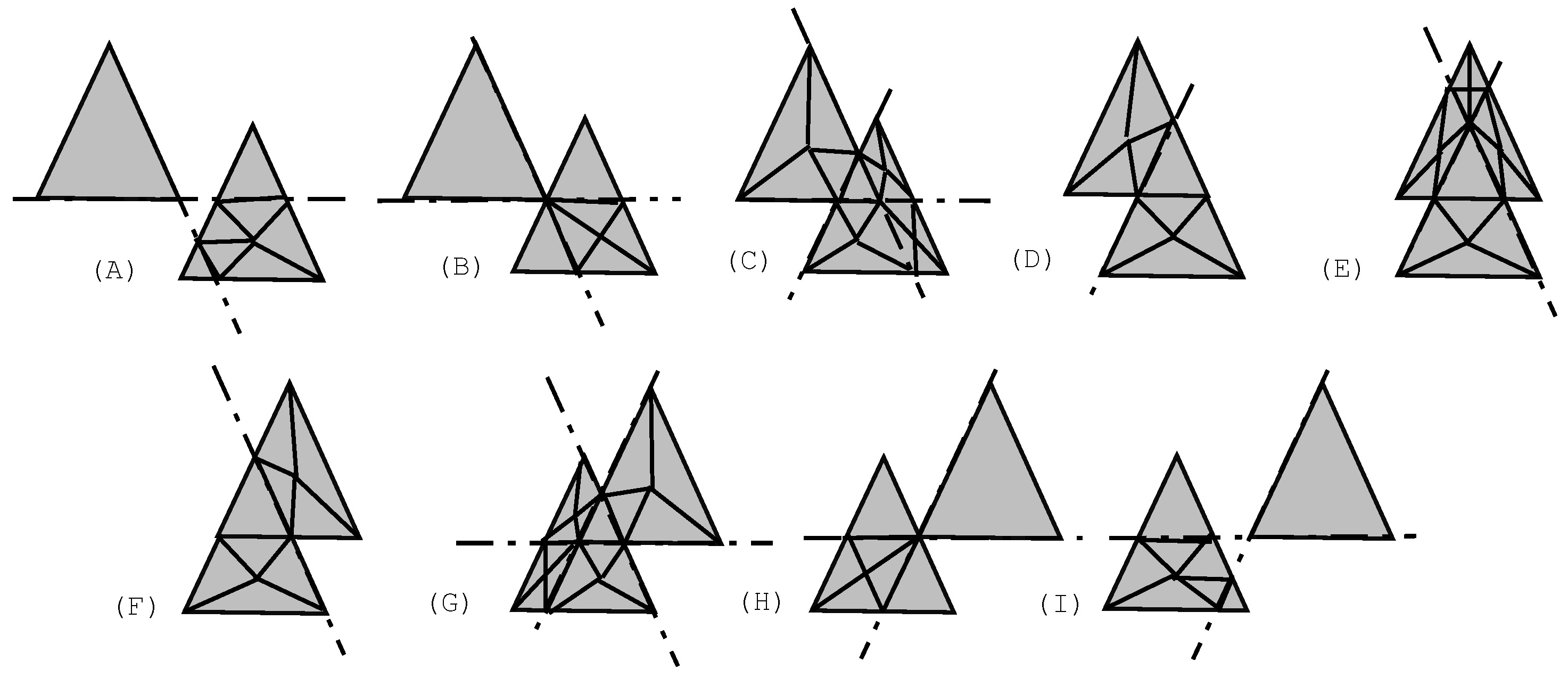
Example 8. Let be a geometric object, where is given as and is given as and f is the mapping given by . Figure 8 shows the snapshots of at time moments (A)
, (B)
, (C)
, (D)
, (E)
, (F)
, (G)
, (H)
and (I).
Let be a geometric object. We assume that the are given as triples of points (i.e., pairs of rational or algebraic numbers), the as structures containing two rational or algebraic numbers and two flags (indicating whether the interval is closed on the left or right side) and, finally, the are affinities given by rational functions, i.e., fractions of polynomials with integer coefficients (that we assume to be given in dense or sparse representation), for .
4.1. The Partitioning Step
Let be a geometric object. In the first step of , the time domain I of , i.e., the convex closure of the union of all the time domains is partitioned in such a way that, for each element of that partition, all its snapshots are -isomorphic.
Below, we refer to the set of lines that intersect the border of in infinitely many points, the set of carriers of the snapshot and denote it , ().
In [
4], we defined the
finite time partition of the time domain of two atomic objects in such a way that for each element
P of
, the carrier sets of each snapshot of
P are topologically equivalent. This definition can easily be extended to an arbitrary number of atomic objects. Also the property stating that the finite time partition exists, still holds in the extended setting.
Definition 10 (Generalized finite time partition). We call a finite time partition of a geometric object any partition of the interval into a finite number of time intervals such that for any (and all ), and are topologically equivalent sets in . ☐
Here, two subsets A and B of are called topologically equivalent when there exists an orientation-preserving homeomorphism h of such that .
The proof of the following property follows the lines of a proof in [
4].
Property 5 (Existence of a generalized finite time partition). Let be a geometric object.There exists a finite time partition of . ☐
We now proceed with the partitioning step of the spatio-temporal triangulation algorithm. In this step, a generalized finite time partition of is computed, using the information of the time-dependent carriers of the atomic objects in . Each time an intersection point between two or more time-dependent carriers starts or ceases to exist, or when intersection points change order along a line, a new time interval of the partition is started. Given three continuously moving lines, the intersection points of the first line with the two other lines only change order along the first line, if there exists a moment where all three lines intersect in one point. Algorithm 2 describes the partitioning step in detail.
We will show later that the result of the generalized finite time partition is a set of intervals during which all snapshots are -isomorphic. This partition is, however, not the coarsest possible partition having this property, because there might be atomic objects that, during some time, are completely overlapped by other atomic objects. Therefor, we will later, after the triangulation step, again merge elements of the generalized finite time partition, whenever possible.
We illustrate Algorithm 2 on the geometric object of Example 8.
Example 9. Recall from Example 8 that , where is given as and is given as and f is the affinity mapping triples to pairs .
We now illustrate the partitioning algorithm on input . First, the list χ will contain the time moments 0 and 4. The list will contain six elements. Table 4 shows these segments and the formulas describing their time-dependent carriers. All pairs of segments have an intersection that exists always, except for the pairs , and . The intersections of with and with exist only at respectively , . The segments and never intersect. Of all possible triples of carriers, only two triples have a common intersection within the interval . The carriers of , and intersect at and the carriers of , and intersect at . The partitioning step will hence return the list | Algorithm 2 Partition (Input: , Output: ) |
- 1:
Let (with ) be a sorted list of time moments that appear either as a begin or endpoint of for any of the objects , . - 2:
. - 3:
for all atomic objects do - 4:
Add the new atomic objects , and to , where , and are the boundary segments of . - 5:
end for - 6:
for all pairs of objects and of do - 7:
if then - 8:
Compute the end points of the intervals during which the intersection of the carriers of both time-dependent line segments does exist. Add those such end points that lie within the interval to , in a sorted way. - 9:
end if - 10:
end for - 11:
for all triples of objects , and of do - 12:
if then - 13:
Compute the end points of the intervals during which the carriers of the three time-dependent line segments intersect in one point. Add those such end points that lie within the interval to , in a sorted way. - 14:
end if - 15:
end for - 16:
Return .
|
We analyze both the output complexity and sequential time complexity of the partition step. First remark that the product of ℓ univariate polynomials of degree d is a polynomial of degree . Let the transformation function of an atomic object consists of rational coefficients, being fractions of polynomials of degree at most d. It follows that the time-dependent line segments and carriers can be defined using fractions of polynomials in t of degree . Also, the time-dependent intersection point of two such carriers and the time-dependent cross-ratio of an intersection point compared to two moving end points of a segment, can be defined using fractions of polynomials in t of degree .
Property 6 (Partition: output complexity). Given a geometric object consisting of n atomic objects. Let d be the maximal degree of any polynomial in the definition of the transformation functions . The procedure Partition, as described in Algorithm 2, returns a partition of containing elements.
Proof. It is clear that the list contains elements after Line 1 of Algorithm 2. Indeed, at most two elements are added for each atomic object. The list will contain at most elements. For each atomic object with a reference object that is a “real” triangle, 3 elements will be added to . In the case that one or more corner points coincide, one or two objects will be added to .
Now we investigate the number of time moments that will be inserted to while executing the for-loop starting at Line 6 of Algorithm 2. The intervals during which the intersection of two time-dependent carriers exists are computed. The intersection of two time-dependent line segments doesn’t exist at time moments where the denominator of the rational function defining it is zero. Because this denominator always is a polynomial P in t, it has at most zeroes, where denotes the degree of P. Accordingly, at most elements will be added to . Hence, in total, time moments are added in this step.
For the intersections of three carriers, a similar reasoning can be used. Hence, during the execution of the for-loop starting at Line 11 of Algorithm 2, elements are added to .
We can conclude that the list will contain elements. ☐
Now we analyze the time complexity of
Partition. We first point out that finding all roots of an univariate polynomial of degree
d, with accuracy
can be done in time
[
35]. We will use the abbreviation
for the expression
. Note also that, although the product of two polynomials of degree
d is a polynomial of degree
, the computation of the product takes time
. To keep the proofs of the complexity results as readable as possible, we will consider the complexity of any manipulation on polynomials (computing zeros, adding or multiplying) to be
, where a precision of
is obtained.
Property 7 (Partition: computational complexity). Given a geometric object consisting of n atomic objects. Let d be the maximal degree of any polynomial in the definition of the transformation functions and let ϵ be the desired precision for computing the zeros of polynomials. The procedure Partition, as described in Algorithm 2, returns a partition of in time .
Proof. Let be a geometric object. Let d be the maximum degree of any of the polynomials used in the definition of the functions .
Constructing the initial list , on Line 1, takes time (it is well known that the inherent complexity of sorting a list of n elements is ). Computing the set can be done in time : all n elements of are considered, and the time needed to copy the transformation functions depends on the maximal degree the polynomials defining them have. Recall that contains at most elements.
The first for-loop, starting at Line 6 of Algorithm 2 is executed times. One execution of its body takes . Indeed, computing the formula representing the time-dependent intersection, checking whether its denominator is always zero and finding the zeros of the denominator (a polynomial of degree linear in d) have all time complexity . Therefor, the first for-loop takes time in total.
The second for-loop has time complexity . The reasoning here is the same as for the previous for-loop.
Finally, sorting the list , which contains elements at the end, requires .
If we summarize the complexity of all the separate steps, we obtain . ☐
We now proceed with the triangulation step.
4.2. The Triangulation Step
Starting with a geometric object , the partitioning algorithm identifies a list of time moments that is used to partition the time domain of into points and open intervals. For each element in that partition (point or open interval), we now triangulate the part of restricted to that point or open interval.
The triangulation of the snapshots of at the time moments in is straightforward. For each of the time moments of , the spatial triangulation method is applied to the snapshot . For each of the triangles in , an atomic object is constructed with as reference object, the singleton as time domain and the identity as its transformation function.
The triangulation of the parts of
restricted to the open intervals in the time partition requires a new technique. We can however benefit from the fact that throughout each interval, all snapshots of
have an
-isomorphic triangulation. For each of the open intervals
defined by two subsequent elements of
, we compute the snapshot at the middle
of
and its triangulation
. Each triangle boundary segment that contributes to the boundary of
at time moment
, will also contribute to the boundary of
at the snapshot of
at any time moment
. So, the moving line segment can be considered a boundary segment throughout
. If two carriers of boundary segments intersect at time moment
, the intersection of the moving segments will exist throughout
, and so on. Therefor, we will compute the spatial triangulation of the snapshot
using the procedure
, but we will copy every action on a point or line segment at time moment
on the moving point of line segment of which the point or segment is a snapshot. The triangles returned by the spatial triangulation algorithm when applied to
will be reference objects for the atomic objects, returned by the spatio-temporal triangulation algorithm. These atomic objects exist during the interval
. Knowing the functions representing the time-dependent corner points of the triangles (because of the copying), together with the time interval and the reference object, we can deduce the transformation function and construct atomic objects (the formula computing this transformation was given in [
4]).
Next, a detailed description of the spatio-temporal triangulation is given in Algorithm 3. In this description of the spatio-temporal triangulation procedure, we will use the data type Points which is a structure containing a (2-dimensional) point (represented using a pair of real numbers), a pair of rational functions of t (a rational function is represented using a pair of vectors of integers, denoting the coefficients of a polynomial), representing a moving point, and finally a time interval (represented as a pair of real numbers and two flags indicating whether the interval is open or closed at each end point). We will only use or fill in this time information when mentioned explicitly. Given an element of type Points, we address the point it stores by , the functions of time by and respectively, and the begin and end point of the time interval by and . The flags and are true when the interval is closed at its begin or end point respectively. A pair of elements of the type Points is denoted an element of the type Segments.
We again illustrate the spatio-temporal triangulation algorithm on the geometric object of example 8.
| Algorithm 3 Triangulate (Input: , Output = ) |
- 1:
for all time moments , of do - 2:
for all triangles T in do - 3:
return the atomic element . - 4:
end for - 5:
end for - 6:
Let be the list containing all atomic objects , sorted by the begin points of their time domains. - 7:
Let be a list of elements of the type Segments, . - 8:
for all pairs , , in do - 9:
:= . - 10:
Remove all elements of for which . - 11:
for all elements remaining in do - 12:
:= , . - 13:
end for - 14:
for all in for which is do - 15:
Construct three Points , and such that , , and and respectively contain and (). - 16:
Construct three Segments , and , containing two different elements from the set . Add them to . - 17:
end for - 18:
Compute the set of elements of the type Segments, using only the constant point information of the elements of . Meanwhile, construct the subdivision . - 19:
Compute the convex hull , using only the constant point information of the elements of , a list of elements of the type Points. - 20:
Construct DCEL, where each half-edge (resp. origin) is now an element of the type Segments (resp. Points). Use as a bounding box. Each time the intersection of two constant carriers is computed, also compute the formula representing the moving intersection point. - 21:
while there are any unvisited Segments in DCEL left do - 22:
Compute the list Elist of Segments that form a convex polygon. Compute the Points structure containing both the constant and time-dependent center of mass of that polygon - 23:
if belongs to a face of then - 24:
for all elements of E list do - 25:
Output the atomic object , where S is the triangle with corner points , and and I is . The transformation function f is computed using the functions , , , , and . - 26:
end for - 27:
end if - 28:
end while - 29:
end for
|
Example 10. Recall from Example 8 that , where is given as and is given as and f is the affinity mapping triples to pairs .
From Example 9, we recall that the output of the procedure Partition on input was the list .
The triangulation of the snapshots at one of the time moments in χ are shown in Figure 9. To keep the example as simple as possible, we did not further triangulate convex polygons that are triangles already. The open intervals to be considered are , , , and . We illustrate the triangulation of the interval . During the time interval , the triangulation will always look like the one shown in Part (A) of Figure 9. Hence, will not change, and will be partitioned into seven triangles. The top one will not change, so the atomic object will be part of the output. For the others, we have to compute the time-dependent intersections between the carriers and afterwards apply the formula from [4]. We illustrate this for . the snapshot of at the middle point of is the triangle with corner points , and . Its time-dependent corner points are , and . Solving the matrix equationgives the transformation function that maps triples to pairs . We also give the output complexity and time complexity for this triangulation step.
Property 8 (Triangulation step: output complexity). Given a geometric object consisting of n atomic objects and a finite partition χ of its time domain into k time points and open intervals. The procedure Triangulation, as described in Algorithm 3, returns atomic objects.
Proof. The number of atomic objects returned by the triangulation procedure for one time interval is the same as the number of triangles returned by the spatial triangulation method on a snapshot in that interval. We know from Property 2 that the number of triangles in the triangulation of a snapshot composed from n triangles is . Since their are moments and intervals for which we have to consider such a triangulation, or a slightly adapted version of it, this gives .☐
Property 9 (Triangulation step: computational complexity). Let a geometric object consisting of n atomic objects and a finite partition χ of its time domain into k time points and open intervals be given. Let d be the maximal degree of any polynomial in the definition of the transformation functions and let ϵ be the desired precision for computing the zeros of polynomials. The procedure Partition, as described in Algorithm 2, returns a spatio-temporal triangulation of in time .
Proof. The first for-loop of Algorithm 3 is executed k times. The time needed for computing the snapshot of one atomic object at a certain time moment is . The spatial triangulation algorithm runs in time , as was shown in Property 3. So we can conclude that the body of the first for-loop needs time. Sorting the atomic objects by their time domains takes .
The second for loop is executed once for each open interval, defined by two consecutive elements of . In the body of this loop, first the list is updated. Each insertion or update takes time . At most all objects are in the list , so this part, described in the Lines 10 through 18 of Algorithm 3, needs time . The next part, described in the Lines 19 through 29 essentially is the spatial triangulation algorithm, but, any time the intersection between two line segments is computed, also the rational functions defining the time-dependent intersection of their associated time-dependent line segments are computed. Computing those functions takes time . So the second part of the body of the second for loop requires .
If we add up the time complexity of two for-loops and the sorting step, we have , which is . ☐
4.3. The Merge Step
We already mentioned briefly in the description of the partitioning step that the partition of the time domain, as computed by Algorithm 2, might be finer than necessary. The partitioning algorithm takes into account all line segments, also those of objects that, during some time span, are entirely overlapped by other objects. To solve this, we merge as much elements of the time partition as possible.
The partition of the time domain is such that the merging algorithm will either try to merge a time point and an interval of the type or , or two different intervals of the type and or and . Here, we use the (unusual) notational convention that ( and ) can be either [ or ].
The simplest case is when a time moment and an interval have to be tested. Assume that these are and , respectively. These elements can be merged if there is a one to one mapping M from the atomic elements with time domain to those with time domain in the triangulation. Furthermore, for each pair of atomic objects and , if and only if the left limit . We note that, for rational functions f of t, equals , provided that is in the domain of f. We also note that is in the domain of f only if all coefficients of the transformation function f are well-defined for and if the determinant of f is nonzero for .
When two intervals are to be merged, the procedure involves some more tests. Let
and
be the intervals to be tested. First, we have to verify that for each atomic object
,
is in the domain of
and that for each atomic object
,
is in the domain of
. Second, we have to test whether
can be continuously expanded to
. This involves the same tests as for the simple case where an interval and a point are tested. Finally, two atomic object can only be merged if the combined atomic object again is an atomic object. This means that, if
would have been chosen as a reference object for
, then
would be equal to
, and vice versa. This can be tested ([
4]).
This merge step guarantees that the atomic objects exist maximally and that the resulting triangulation is the same for geometric objects that represent the same spatio-temporal object. Algorithm 4 shows this merging step in detail.
| Algorithm 4 Merge (Input: , Output: |
- 1:
Sort all atomic objects by their time domains. - 2:
Let be the list . - 3:
Let be the first element of and the second. - 4:
while there are any elements in left do - 5:
(resp. ) is the set of all objects having (resp. ) as their time domain. - 6:
if is a point then - 7:
Preprocess the reference objects of the elements of such that we can search the planar subdivision they define. - 8:
let Found be true. - 9:
for all objects in do - 10:
Check whether is part of the time domain of . - 11:
Compute their snapshot at time (which is a triangle ). - 12:
Do a point location query with the center of mass of in and check whether the triangle found in has the same coordinates as . If not, Found becomes false. - 13:
if Found is false then - 14:
break; - 15:
end if - 16:
end for - 17:
if found is true then - 18:
remove all elements of from and extend the time domain of all elements of to . - 19:
and is the next element of if any exists. - 20:
else - 21:
and is the next element of , if any exists. - 22:
end if - 23:
else - 24:
if is a point then - 25:
do the same as in the previous case, but switch the roles of and . - 26:
else - 27:
Let be the element of the form and the one of the form . - 28:
Check whether and can be merged. - 29:
if this can be done then - 30:
Check for each pair of matching atomic objects whether their transformation functions are the same ([ 4]). - 31:
end if - 32:
end if - 33:
end if - 34:
end while
|
We illustrate Algorithm 4 on the geometric object of Example 8.
Example 11. Recall from Example 8 that , where is given as and is given as and f is the linear affinity mapping triples to pairs .
From Example 9, we recall that the output of the procedure partition on input was the list . This resulted in a partition of the interval consisting of the elements , , , , , , , , , and . For each of these elements, (a snapshot of) their triangulation is shown in Figure 9. During the merge step, the elements and of the time partition will be merged.
It is straightforward that the output and input of the merging algorithm have the same order of magnitude. Indeed, it is possible that no intervals are merged, and hence no objects. We discuss the computational complexity of the algorithm next. Note that the complexity is expressed in terms of the size of the input to the merging algorithm, which is the output of the spatio-temporal triangulation step.
Property 10 (Merge step: computational complexity). Given a geometric object , which is the output of the triangulation step, and a finite partition χ of its time domain into K time moments and open intervals. Let d be the maximal degree of any polynomial in the definition of the transformation functions and let ϵ be the desired precision for computing the zeros of polynomials. The procedure Merge, as described in Algorithm 4, merges the atomic objects in in time .
Proof. Sorting all atomic objects by their time domains can be done in time . Computing the list can be straightforwardly done in time . This list will contain elements. We assume that (in case the merging algorithm is not applied). The while-loop starting at Line 4 of Algorithm 4, is executed at most times. Indeed, at each execution of the body of the while-loop, one new element of is considered. The if-else structure in the body of the while-loop distinguishes three cases. All cases have the same time complexity, as they are analogous. We explain the first case in detail.
The number of atomic objects having the same time domain is of the order of magnitude of
. This follows from Property 8. The preprocessing of the snapshot takes
time [
33]. The for-loop, starting at Line 9 of Algorithm 4 is executed at most
times. The time needed for checking whether an atomic object exists at some time moment and computing the snapshot (a triangle) is
. Because of the preprocessing on the snapshot at time moment
, testing the barycenter of the triangle against that snapshot can be done in
time [
33]. In case the snapshots are the same, adjusting the time domains of all atomic objects takes time
. Summarizing, the time complexity of the first case is
.
Combining this with the fact that the while-loop is executed times, and the time complexity of the first two steps of the algorithm, we get an overall time complexity of . ☐
Finally, the spatio-temporal triangulation procedure combines the partition, triangulation and merging step. Algorithm 5 combines all steps.
The following property follows from Property 6 and Property 8.
Property 11 (: output complexity). Given a geometric object consisting of n atomic objects. Let d be the maximal degree of any polynomial in the definition of the transformation functions . The spatio-temporal triangulation method , as described in Algorithm 5, returns atomic objects.
| Algorithm 5 (Input: , Output: ) |
- 1:
= Partition(O); - 2:
= Triangulate(, ); - 3:
if has more than one element then - 4:
= Merge(, ); - 5:
return . - 6:
else - 7:
return . - 8:
end if
|
The next property follows from Property 7, Property 9 and Property 10.
Table 5 summarizes the time complexity of the different steps.
Property 12 (: computational complexity). Given a geometric object consisting of n atomic objects. Let d be the maximal degree of any polynomial in the definition of the transformation functions and let ϵ be the desired precision for computing the zeros of polynomials. The spatio-temporal triangulation method , as described in Algorithm 5, returns a spatio-temporal triangulation of in time .
We now show that Algorithm 5 describes an affine-invariant spatio-temporal triangulation method. We remark first that the result of the procedure is a spatio-temporal triangulation. Given a geometric object . It is clear that each snapshot of is a spatial triangulation. Also, . This follows from the fact that the time partition covers the whole time domain of and that the method produces a spatial triangulation.
Property 13 ( is affine-invariant). The spatio-temporal triangulation method , described in Algorithm 5, is affine-invariant.
Proof. (Recall Definition 6 for affine-invariance.) Let and be geometric objects for which for each moment in their time domains, there is an affinity such that .
It follows from the construction of the spatio-temporal triangulation that and also . The property now follows from the affine-invariance of the spatial triangulation method . ☐
The following corollary follows straightforwardly from Property 13:
Corollary 1. Let and be two geometric objects such that there is an affinity such that, for each moment in their time domains holds. Then, for each atomic element of , the element belongs to . ☐
This shows that the partition is independent of the coordinate system used to represent the spatio-temporal object. The affine partitions of two spatio-temporal objects that are affine images of each other only differ in the coordinates of the spatial reference objects of the atomic objects.
Remark also that, in practice, either most of the original objects have the same time domain, making the number of intervals in the partition very small, or all different time domains, which greatly reduces the number of objects existing during each interval. So, in practice, the performance will be better than the worst case suggests.
5. Applications
We now describe some applications that we believe can benefit from the triangulation described in Algorithm 5. We first say what we mean by a spatio-temporal database.
Definition 11. A spatio-temporal database is a set of geometric objects. ☐
For this section, we assume that each atomic object is labelled with the id of the geometric object it belongs to.
5.1. Efficient Rendering of Objects
When a geometric object that is not in normal form has to be displayed to the user, there are two tasks to perform. First, the snapshots of the geometric object at each time moment in the time domain of the object have to be computed. This can be done in a brute force way by computing the snapshots of all atomic objects. Since some will be empty, this approach might lead to a lot of unnecessary computations. Another algorithm could keep track of the time domains of the individual atomic objects and keep a list of active ones at the moment under consideration, which has to be updated every instant. If the geometric object is in normal form, the atomic objects can be sorted by their time domains, and during each interval in the partition of time domain, the list of active atomic objects will remain the same.
The second task is the rendering of the snapshot. If the geometric object is not in normal form, the snapshots of the atomic objects overlap, so pixels will be computed more than once. Another solution is computing the boundary, but this might take too long in real-time applications. When a geometric object is in normal form, no triangles overlap, so each pixel will be computed only once.
5.2. Moving Object Retrieval
The triangulation provides a means of automatic affine invariant feature extraction for moving object recognition. Indeed, the number of intervals in the time domain indicates the complexity of the movement of the geometric object. This can be used as a first criterium for object matching. For objects having approximately the same number of intervals in their time domains, the snapshots at the middle of each time interval can be compared. If they are all similar, which can be, for example, defined as
-isomorphic, the objects match. Or, if more exact comparison is needed, one can extract an affine-invariant description from the structure of the elements of the triangulation of the snapshot (see also
Section 5.6).
5.3. Surveillance Systems
In some applications, e.g., surveillance systems, it is important to know the time moments when something changed, when some discontinuity appeared. This could mean that an unauthorized person entered a restricted area, for example, or that a river has burst its banks. Triangulating the contours of the recorded images and reporting all single points and end points of intervals of the partition of the time domain indicates all moments when some discontinuity might have occurred.
5.4. Precomputing Queries
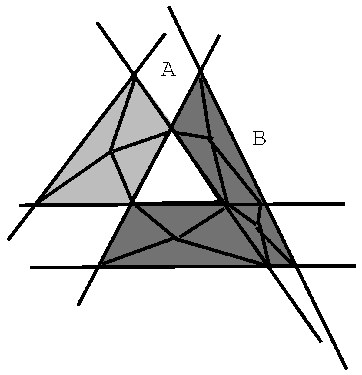
If we do not triangulate each geometric object in a database separately, but use the contours of all geometric objects together in the triangulation, the atomic objects in the result will have the following nice property. For each geometric object in the original database, an atomic object will either belong to (or be a subset of) it entirely, or not at all. This means that we can label each element of the spatio-temporal triangulation of the database with the set of id’s of the geometric objects it belongs to. We illustrate this for the spatial case only in
Figure 10. Suppose we have two triangles
A and
B. The set
A is the union of the light grey and white parts of the figure, the set
B is the union of the dark grey and white parts of the figure. After triangulation, we can label the light grey triangles with
, the white triangle with
, and the dark grey triangles with
.
Using this triangulation of databases in a preprocessing stage, means that the results of queries that ask for set operations between geometric objects are also pre-computed. Answering such a query boils down to checking labels of atomic objects. This means a lot of gain in speed at query time. Indeed, even to compute, for example, the intersection of two atomic objects, one has to compute first the intervals where the intersection exists, and then to consider all possible shapes the intersection can have, and again represent it by moving triangles.
5.5. Maintaining the Triangulation.
If a geometric object has to be inserted into or removed from a database (i.e., a collection of geometric objects), the triangulation has to be recomputed for the intervals in the partition of the time domain that contain the time domain of the object under consideration. This may require that the triangulation in total has to be recomputed.
However, the nature of a lot of spatio-temporal applications is such that updates involve only the insertion of objects that exists later in time than the already present data. In that case, only the triangulation at the latest time interval of the partition should be recomputed together with the new object, to check whether the new data are a continuation of the previous. Also, data is removed only when it is outdated. In that case a whole time interval of data can be removed. Examples of such spatio-temporal applications are surveillance, traffic monitoring and cadastral information systems.
5.6. Affine-Invariant Querying of Spatio-Temporal Databases
An interesting topic for further work is to compute a new, affine-invariant description of geometric objects in normal form, that does not involve coordinates of reference objects. The structure of the atomic objects in the spatio-temporal triangulation can be used for that. Once such a description is developed, a query language can be designed that asks for affine-invariant properties of objects only.


