3.2. Buffer-Based Service Level Analysis
The scope of services is an important aspect of assessing service capabilities, which reflects the range of greenway services. Therefore, to evaluate the service capacity of urban greenways, it is necessary to analyze its scope of services. The buffer-based service level analysis method can effectively determine the regional scope, population range and residential area of linear feature services. Thus, this article uses this method from the perspective of the scope of service to evaluate the urban greenway service capacity.
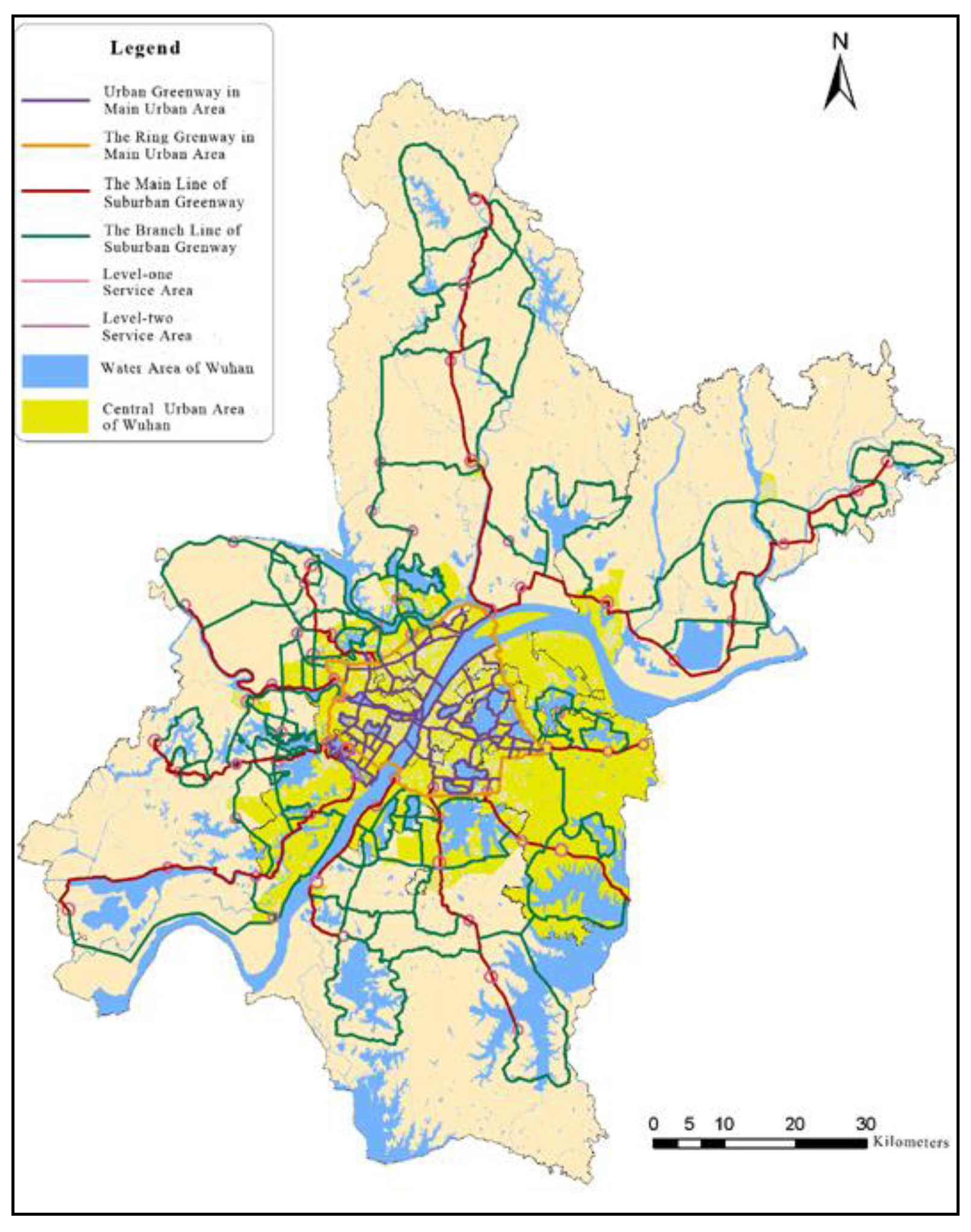
According to the time–cost planned in the greenway system planning in Wuhan stated in
Section 2, the time of arrival can be assigned for each class of greenway. Level 1 greenways are located in the main urban area, and mostly consist of community greenways. Therefore, the arrival time range of Level 1 greenways was set to 5–10 min. The Level 2 greenway is the ring greenway in the main urban area, which belongs to main urban greenways. Thus, the arrival time range of the Level 2 greenway was set to 15–20 min. Level 3 greenways are located outside the main urban area and consist of suburban greenways. Therefore, the arrival time range of Level 3 greenways was set to 30–45 min.
After the arrival time range of the three classes of greenway is determined, the greenway service radius can be calculated when the walking speed is provided. Thus, the service radius of each greenway class is computed by assuming that the average walking speed is 1 m/s [Equation (1)]. Apparently, the service radii of Levels 1, 2, and 3 greenways are 600, 1200, and 2700 m, respectively. The service radius is determined as follows:
where
is the service radius of Level
greenway,
is the human average walking speed,
is the upper limit of arrival time of Level
greenway, and
is 1, 2, or 3.
Subsequently, the relative service level value for each class of greenway should be set. The relative service level value can be used to represent the greenway service level. However, the value does not represent the accurate value of greenway service level. This value is simply a reference, which indicates that a high relative service level value corresponds to the service that can be provided by this kind of greenway.
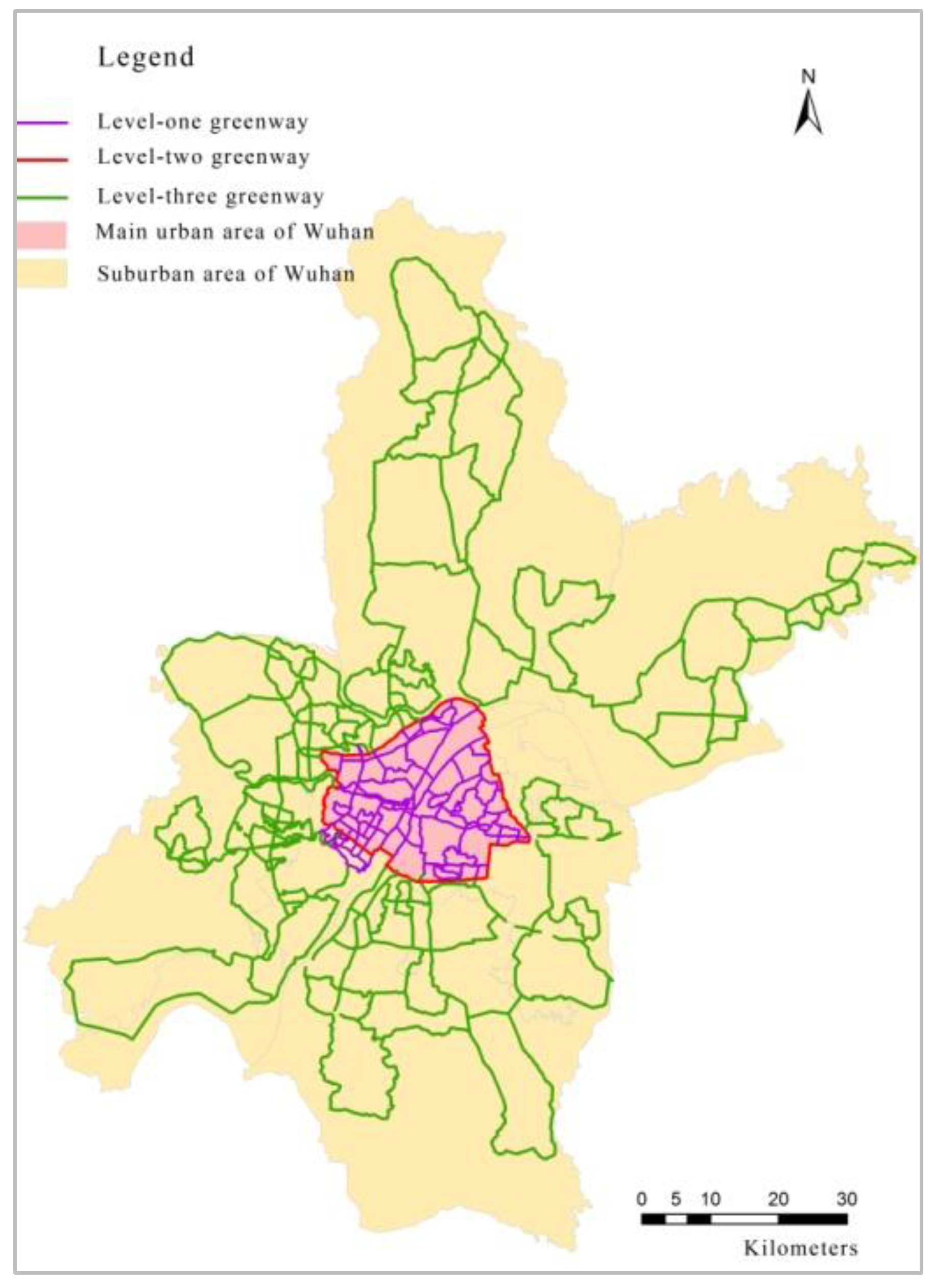
Figure 4 illustrates that Level 1 greenway is located in the main urban area and characterized by an apparent geographical advantage. Thus, improved services can be theoretically provided by Level 1 greenway compared to others. Similarly, the services that can be obtained from Level 2 greenway are better than those from Level 3 greenway. Thus, the relative service level values were assigned to each greenway class in the order of natural numbers. As a result, the relative service level values of Levels 1, 2, and 3 greenways were set to 3, 2, and 1, respectively.
A buffer attribute table can be established through the presented calculation and assignment process (
Table 1). The buffer zones of the greenway service were created on the basis of
Table 1.
The three-level greenway service buffer zones were overlaid by the UNION function of GIS spatial analysis. The relative service level value within the overlapping area was then added to calculate the actual service level value of the greenway buffer. In the relative service level value in
Table 1, the actual service level value is an integer between 1 and 6. The superposition results were then divided into three categories. The service levels were set to III, II, and I when the actual service level values ranged between 1 and 2, 3 and 4, and 5 and 6, respectively. Thus, the distribution map of the greenway service level was obtained (
Figure 5).
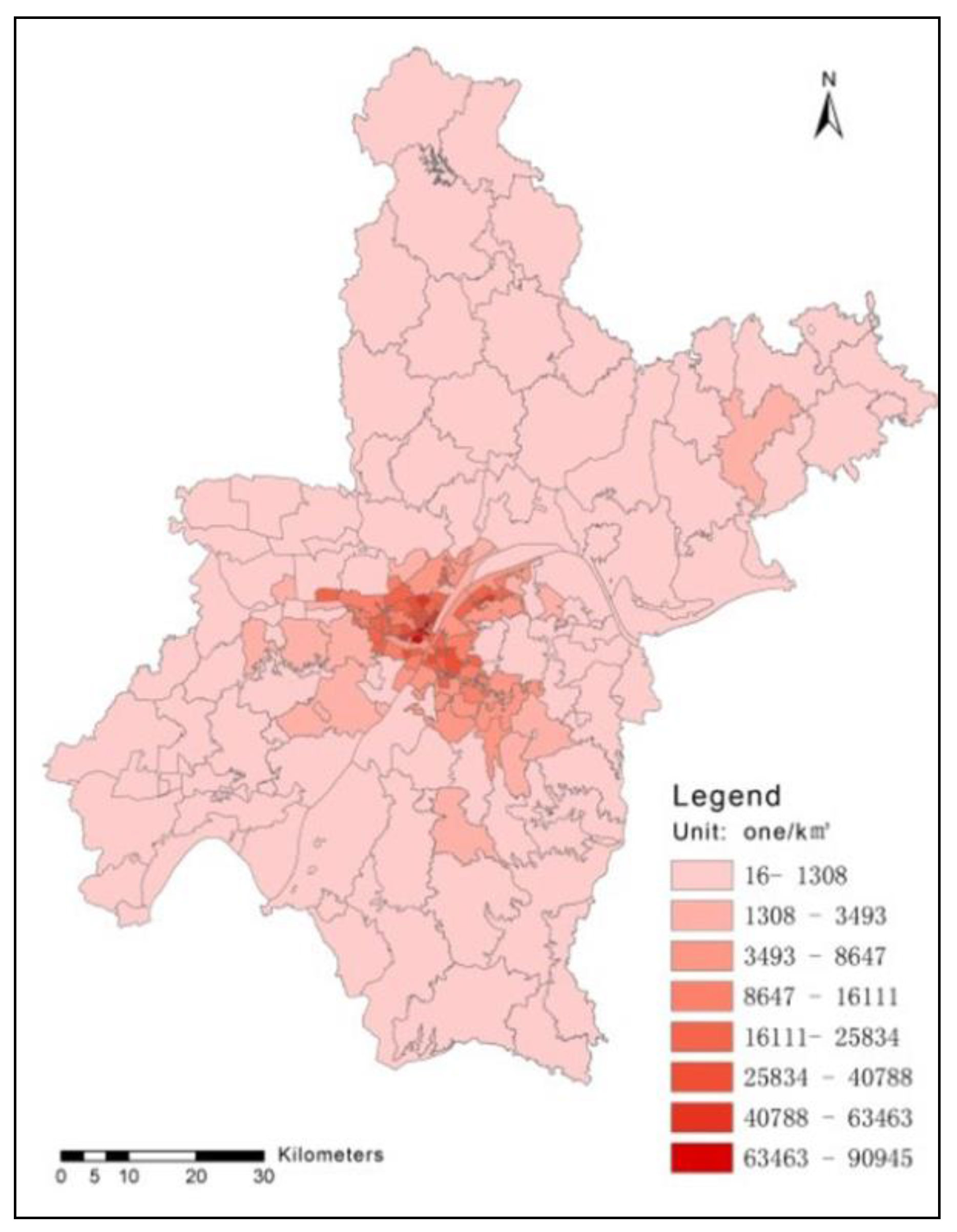
After obtaining the greenway service level data shown in
Figure 5, the population density distribution map was generated using the sixth census, Data of Wuhan. The population density distribution of Wuhan is shown in
Figure 6.
The greenway service level data and population density data were intersected to obtain the demographic information of different service levels by using the intersection function of ArcGIS overlay analysis module. The greenway service level data and the Wuhan residential quarter data were superimposed to obtain the living area statistics in different service levels. The number of urban populations and the area of residential quarters were determined by following the abovementioned detailed steps, and our results indicated that urban greenways can serve the entire city area.
3.3. Minimum Distance-Based Accessibility Analysis
Service convenience is another important aspect of service capability evaluation, and this aspect reflects the convenience of urban residents to utilize greenway services. Therefore, the service convenience of urban greenways should be analyzed to evaluate their service capacity. The reachability analysis method, based on the minimum proximity distance, is based on the distance from the residential area to the green road, which can effectively show the convenience of the greenway service. This method is used in our study on the basis of the service convenience, to evaluate the service capacity of urban greenways.
The minimum distance method represents the accessibility level by considering the distance from the residential quarters to the nearest greenway. This method is based on the assumption that people tend to exercise or spend their leisure times at greenways located close to their living area. Thus, this method is appropriate and commonly used in accessibility analysis [
16].
A rational level division of greenway accessibility should be formed in the implementation stage. In accordance with the Wuhan greenway system planning stated in
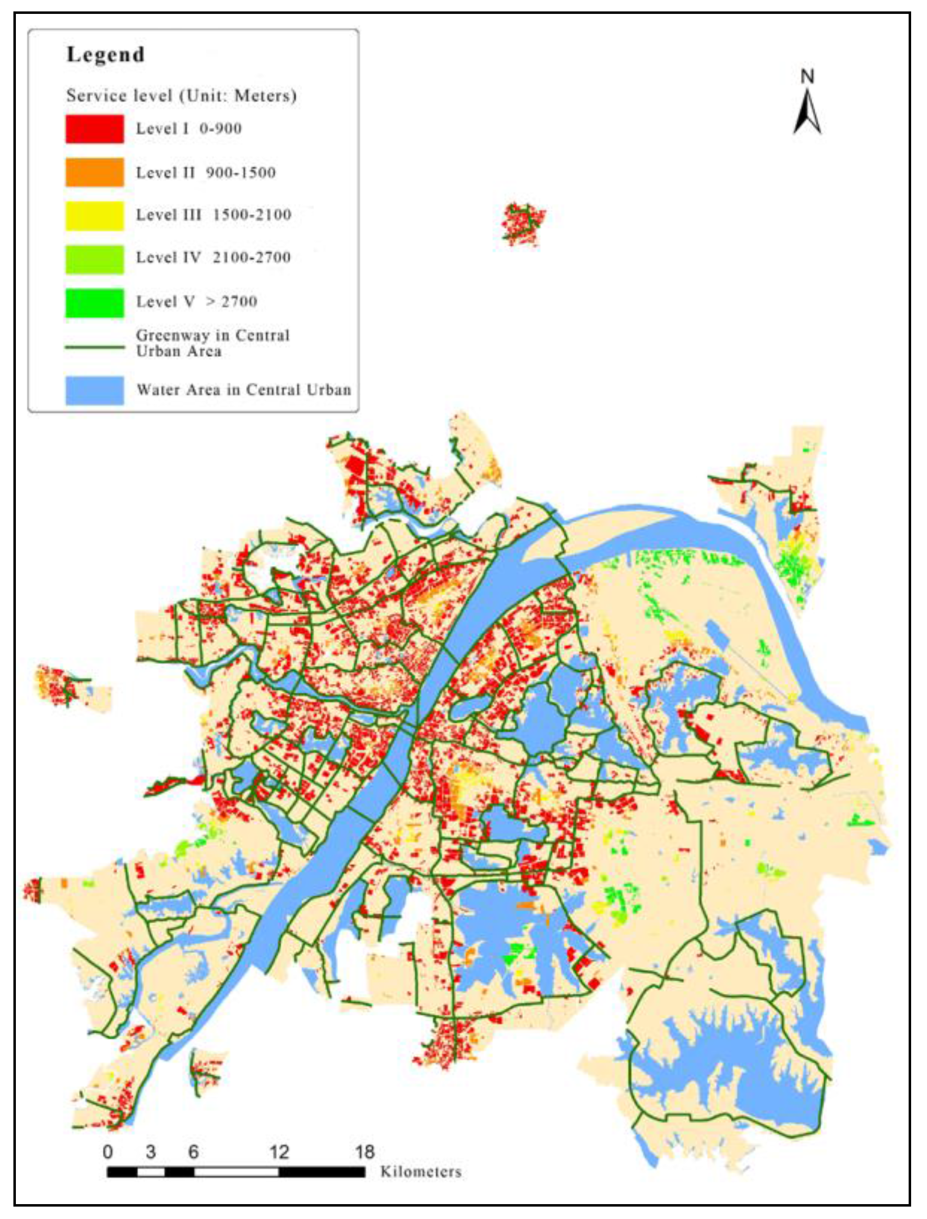
Section 2, the public can reach the greenways in all regions within 5–45 min. A 10 min interval was set for segmentation of the arrival times, to present the accessibility level of greenway. Hence, the total arrival time interval was divided into five segmentations, which consisted of 5–15, 15–25, 25–35, 35–45, and more than 45 min. Based on these arrival time ranges, the normal walking speed is assumed to be 1 m/s. The ranges of reach distance were then determined for each corresponding time segment. These ranges are shorter than 900, 900–1500, 1500–2100, 2100–2700, and longer than 2700 m.
The accessibility level division table can be established by using the presented division and estimation processes (
Table 2). In
Table 2, a short reach distance corresponds to a high accessibility level. Thus, the highest accessibility level is Level I, and the lowest accessibility level is Level V.
In this method, the distance from the residential quarters to the nearest greenway was calculated by using the minimum distance module of ArcGIS. The residential quarters were subsequently divided into different accessibility levels based on the residential quarter data of Wuhan, and the division rules shown in
Table 2. Based on the distribution of residents of Wuhan (shown in
Figure 6), and requirements of different accessibility level in time and distance (shown in
Table 2), we know that the greenway which meets the time and distance requirements of different accessibility levels is mainly located in the main urban area of Wuhan. The obtained distribution thematic map of the greenway accessibility level in main urban area of Wuhan is shown in
Figure 7.
Finally, a statistic of the residential quarter area in different greenway accessibility levels can be performed using the greenway accessibility level data (
Figure 7). Then, the greenway accessibility level data and the population density data were intersected to obtain the demographic information of different accessibility levels. Through these processes, we determined the area of residential quarters and the number of residential population at different levels of accessibility. Obviously, the higher the accessibility level, the more conveniently the residents can reach a greenway from their residential quarters.
3.4. Comprehensive Service Capability Evaluation
Quality of service is another important aspect of service capacity evaluation, and this parameter indicates the actual effect of a greenway service. Therefore, the quality of services should be assessed to evaluate the service capacity of urban greenways. Integrated service capability analysis method combines various influencing factors that can objectively reflect the actual effect of greenway service. This method is used on the basis of service quality perspectives to evaluate the service capacity of urban greenways.
Relevant factors should be defined to evaluate the comprehensive service capability of an urban greenway network. In our study, the following factors used to evaluate the comprehensive service capability of the greenway network of an urban area are proposed: urban traffic convenience, public and government service facilities surrounding the greenway, urban population density, residential areas, and greenway service level values. The first five factors are called influencing factors. Thus, this study presents a greenway comprehensive service capability model based on regular grids. The calculation formula is given as follows:
where
is the comprehensive service capability of the
i-th grid,
is the population coefficient of the
i-th grid,
is the residential area coefficient of the
i-th grid,
is the public service facility coefficient of the
i-th grid,
is the government service facility coefficient of the
i-th grid,
is the public transport coefficient of the
i-th grid, and
is the greenway service level coefficient of the
i-th grid.
In reality, the service objects of greenways are mainly the residents of urban areas. Among the five influencing factors, population and residential area coefficients represent the number of potential greenway users, which is the main aspect influencing the quality of green service. Public transport, public service facility, and government service facility coefficients correspond to the completeness of greenway service, and their influence on the quality of greenway service is lower than that of population and residential area coefficients. The weight of the main influencing factor is set to 2, because the value range of the influencing factor is at [0, 1] to show the difference of the degree of influence accurately. The weight of the secondary influencing factor is set to 1. In Equation (2), other modest weigh settings are equally acceptable, as long as they do not overstate or diminish the degree of influence.
Six key steps should be performed on the basis of the model shown in Equation (2), to derive the comprehensive service capability of urban greenways.
(1) Regular grid division.
In Step 1, the research area was divided into regular grids with the size of 1 km × 1 km, based on the construction goal of “500 Meters to Reach the Greenbelt, 1000 Meters to Reach the Garden.”
(2) Value statistics of the five influencing factors in each grid cell.
In Step 2, the values of the five influencing factors include the number of population in a grid cell (
), the area of residential quarters in a grid cell (
), the number of public transport points in a grid cell (
), the number of public service points in a grid cell (
), and the number of government service points in a grid cell (
). We suppose that
represents a single grid cell,
represents the population,
represents the area of residential quarters,
represents the position of public transport points,
represents the position of public service points, and
represents the position of government service points. The processes of value statistics were as follows: The first process involves overlaying the regular grid layer to the layers related to the population, residential quarter, public transport, public service, and government service. The second involves calculating the values of the five influencing factors in each grid cell using Equation (3).
In Equation (3), means that the spatial objects are within a grid cell.
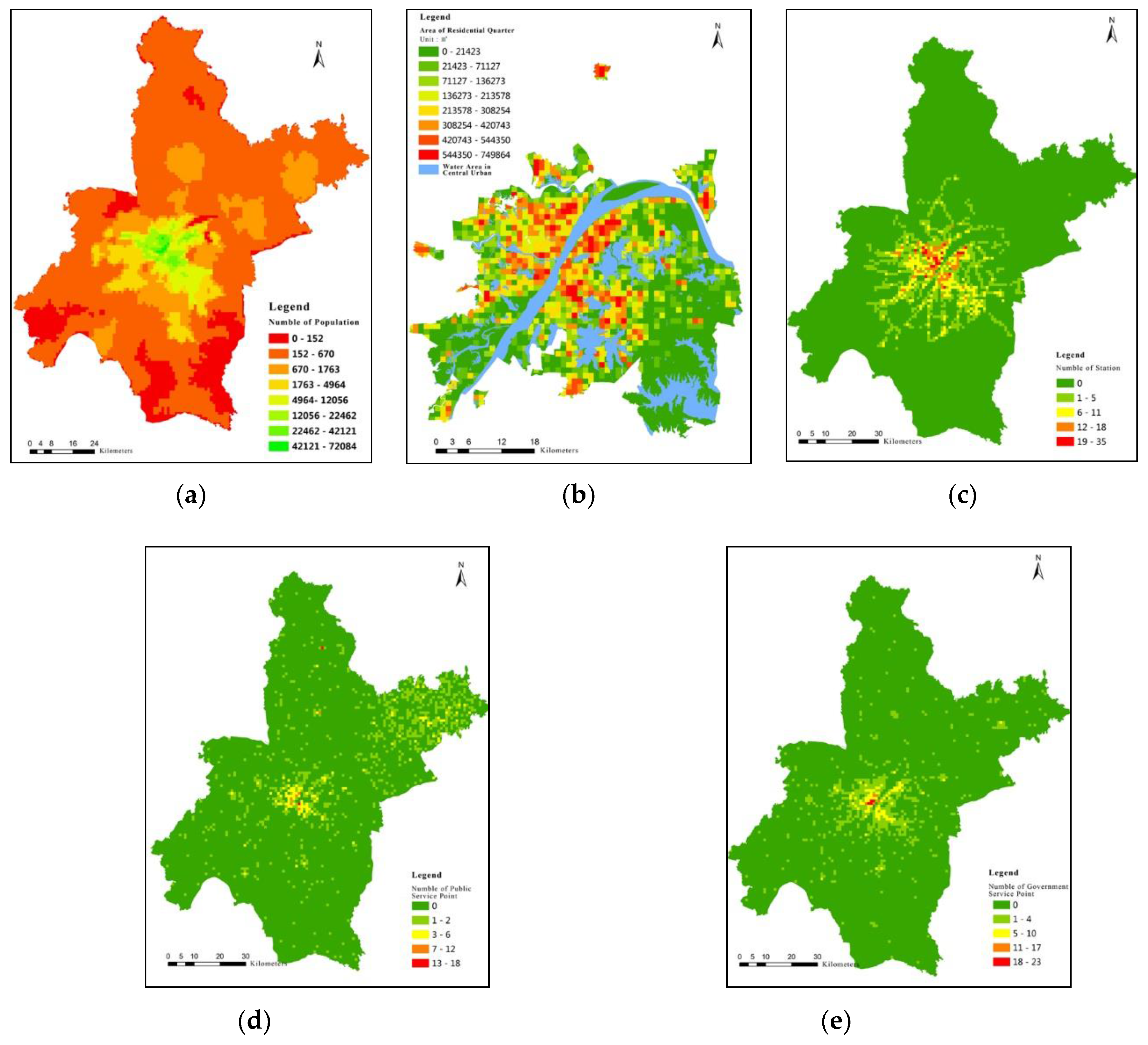
(3) Grading of the five influencing factors.
In Step 3, the thematic map of the distribution of the five influencing factors (
Figure 8) is derived by grading the values of the five influencing factors in each grid cell, which were obtained in Step 2. A high value of a certain influencing factor likely yields a high grade of the corresponding influencing factor. In
Figure 8, the distribution of five different influencing factors indicate that the high-grade areas are concentrated in the urban center. Low-grade areas are widely distributed throughout the suburban areas.
(4) Calculation of the coefficients of the five influencing factors.
In Step 4, weights were assigned to each corresponding grade of each influencing factor in the order of natural numbers (e.g., grade 1 had an assigned weight of 1, grade 2 had an assigned weight of 2) after grading for the five influencing factors. We then normalized the weights to obtain the final coefficients. Equation (4) shows the calculation method of weight normalization.
In Equation (4), represents the coefficient of grade of a certain influencing factor, represents the assigned weight of grade of a certain influencing factor, represents the grade of a certain influencing factor, and represents the highest grade of a certain influencing factor.
(5) Calculation of the greenway service level coefficient.
In Step 5, the greenway service level data, including the actual service level value, obtained in
Section 3.2 were used. First, the regular grid layer and the greenway service level layer (data) were overlaid. Next, the average of the actual service level value in each grid cell was calculated, that is, the average of a certain grid cell was the greenway service level coefficient of that grid cell.
represents a single grid cell,
reflects the greenway service level coefficient of a certain grid cell,
corresponds to one of the actual service level value in a certain grid cell, and
refers to the number of the actual service level value in a certain grid cell. The greenway service level coefficient is calculated using Equation (5).
In Equation (5),
means that the spatial objects are within a grid cell.
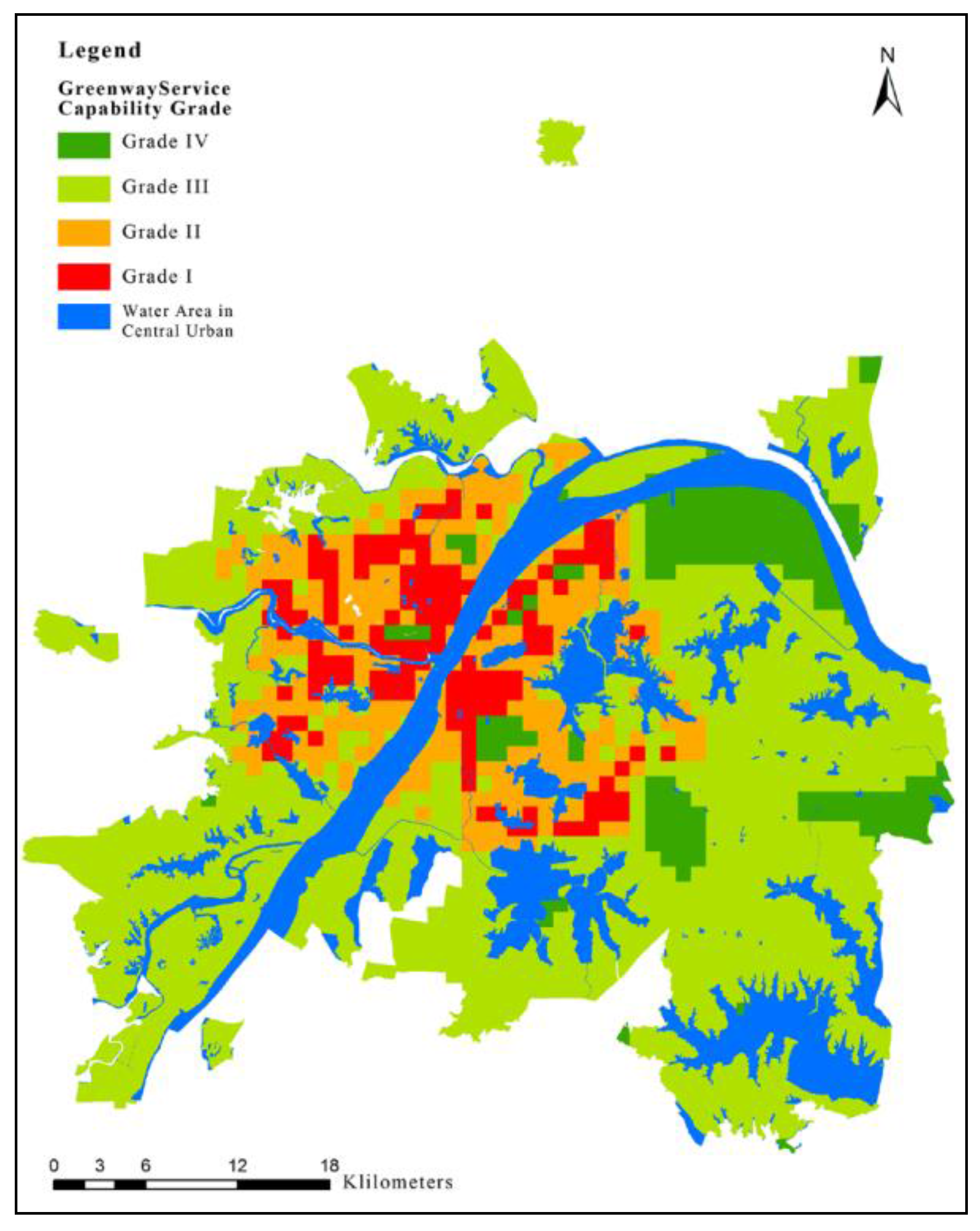
(6) Calculation of the comprehensive service capability value of urban greenways.
In Step 6, the coefficients of the five influencing factors obtained in Step 4, and the greenway service level coefficient obtained in Step 5, were substituted into Equation (2) to derive the comprehensive service capability value of urban greenways in each grid cell. A high value of represents high service quality.


