2.1. Data Field Index Calculation
The feature space is a basic concept in hyperspectral remote sensing studies. Pixels with similar spatial positions are more likely to belong to the same kind of objects than pixels that are far away from each other. In the feature space, the distance between similar pixels is closer and more likely to converge. Mixed pixels are more likely to be located on the boundary between different kinds of objects. However, anomalous endmembers are prone to be located in the sparsest areas in the feature space. A large homogeneous area in an image space has the cluster characteristics of the feature space, while an anomalous endmember appears as an isolated point. Therefore, the traditional preprocessing methods cannot adequately extract abnormal endmembers in large homogeneous areas.
According to the characteristics of physical fields, the structural characteristics of a hyperspectral image in feature space can be described by the data field theory. The data in the feature space are regarded as data particles, which can radiate energy; thus, the entire feature space is projected to the data field space, and each point in the space has a corresponding potential value. Using the field theory from physics as a reference, we introduce the intrinsic interactions of material particles and the corresponding field description to describe an abstract image datum space.
There exist some particles or nuclei of a given mass with a field around them in the space, in which any given object is subject to the force exerted by the other objects. Thereby a data field is determined over the entire space. For static data that do not depend on time, the data field can be considered stable and active. Therefore, given all the intensity vectors or the potential scalars, we can describe the spatial distribution.
From a point within the data field, the pixels are no longer isolated data points. Instead, they represent many particles capable of radiation. A given point radiates energy from itself to the entire area covered by the image. The energy intensity decreases with increasing distance. Any pixel receives energy from the surrounding points; meanwhile, it radiates energy to other points.
The potential energy function is calculated in formula (1) [
23]:
where m ≥ 0 denotes the grey value of a pixel;
k ∈ N denotes the distance index; and
k, which is set to two in this study, represents the Euclidean distance. σ is the impact factor, which is a constant of the data field and describes the potential influence of the pixels on one another. When this factor is small, there is little influence between the pixels, reflecting limited clustering. In such cases, the lines of equal potential also describe independent pixel-centric regions of energy. With increases in the impact factor, increasing interactions between individual data pixels occur, and the line features are closer together. The effects of the impact factor on the endmember extraction tests will be evaluated in the experiments described in
Section 3.
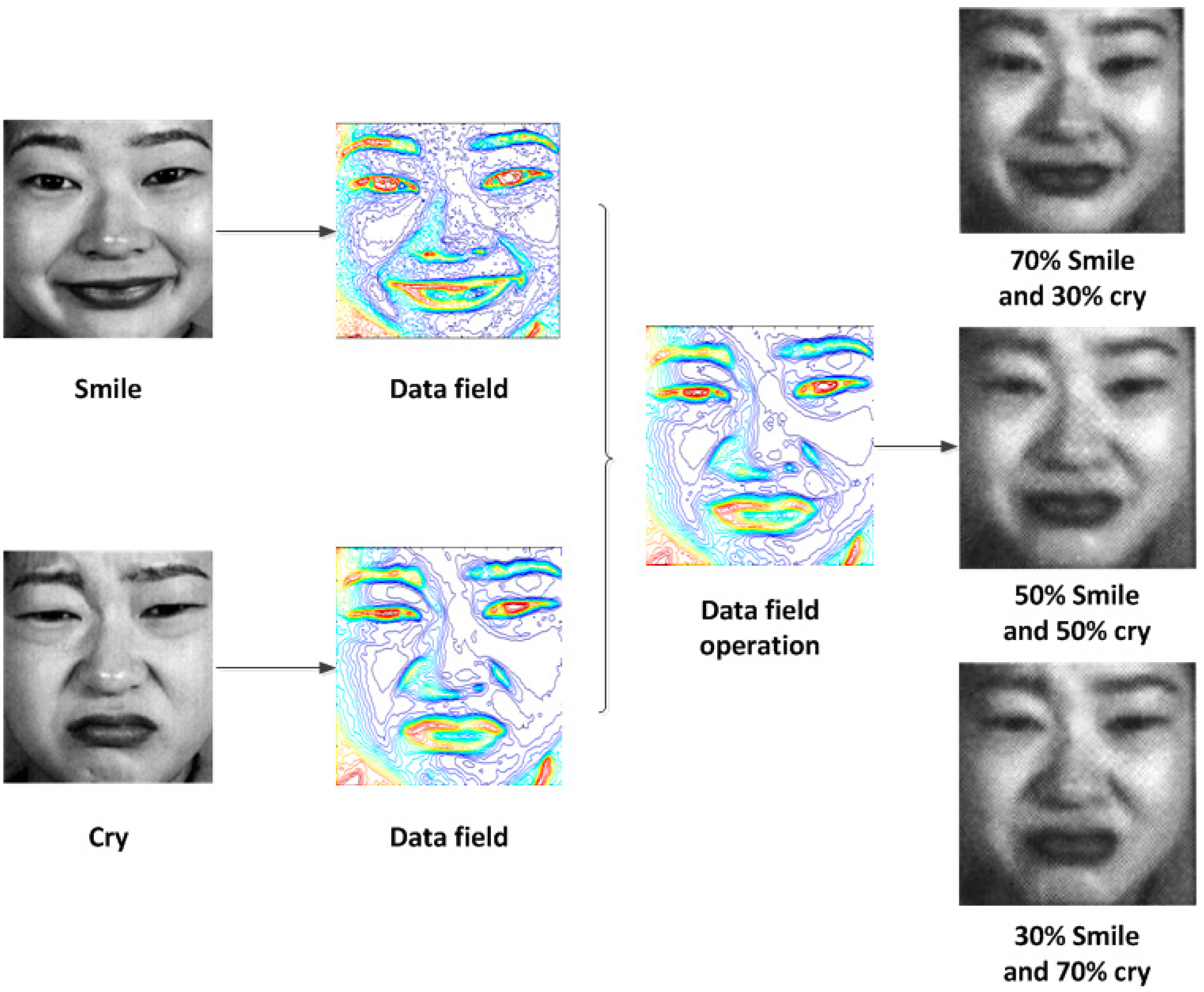
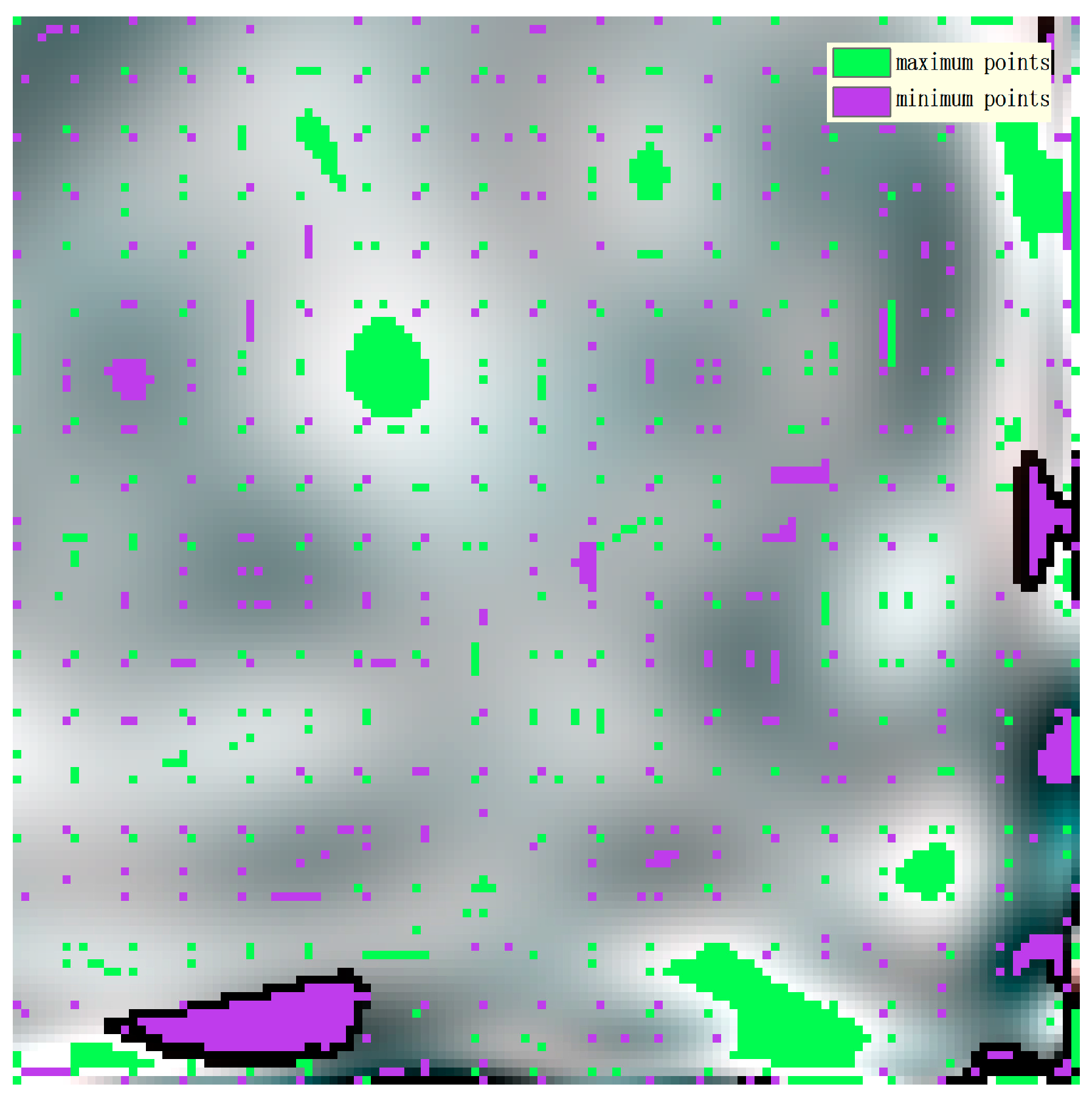
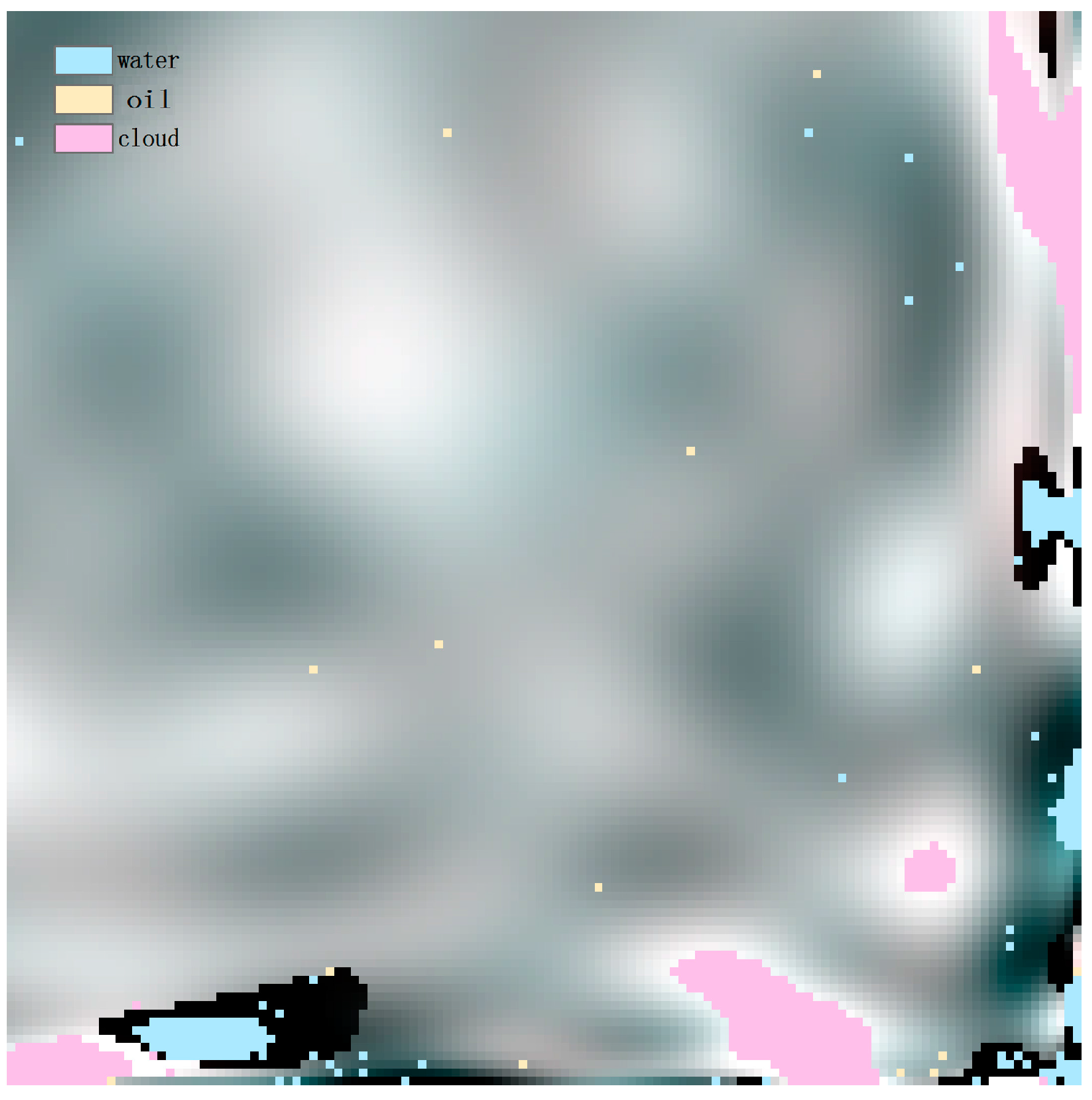
The data field model can effectively and conveniently reflect the distribution of the important feature points (such as the maxima and minima in the data field space) of the original image in different characteristic spaces. Using the field operation of the data field, the original image can be easily transformed through the extraction of feature points. Take a face for example, which can easily demonstrate the function of the data field model, as shown in
Figure 2.
Different spatial and spectral characteristics in the local region result in different spatial distributions and different data fields associated with each pixel vector in the image space. We used the potential energy as the feature to extract from the characteristics of the data field, thus achieving the purpose of the endmember extraction preprocessing.
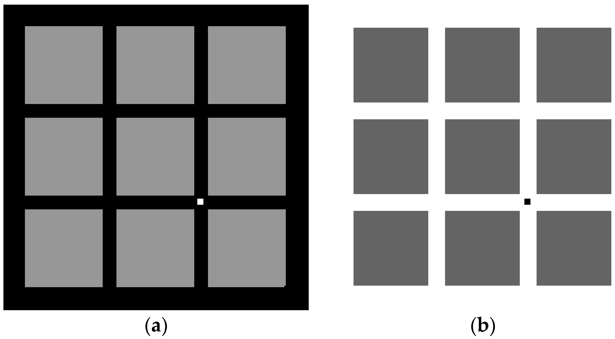
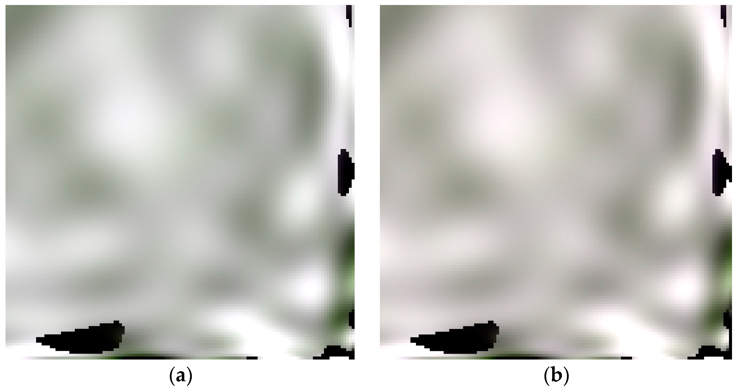
To more deeply explore the characteristics of an image data field, this paper studied the data field properties of central pixels and their neighbouring pixels in an image. We simulated a grid with a background value of
= 0 and a foreground value of
= 150, and another grid with a background value of
= 255 and a foreground value of
= 100, as shown in
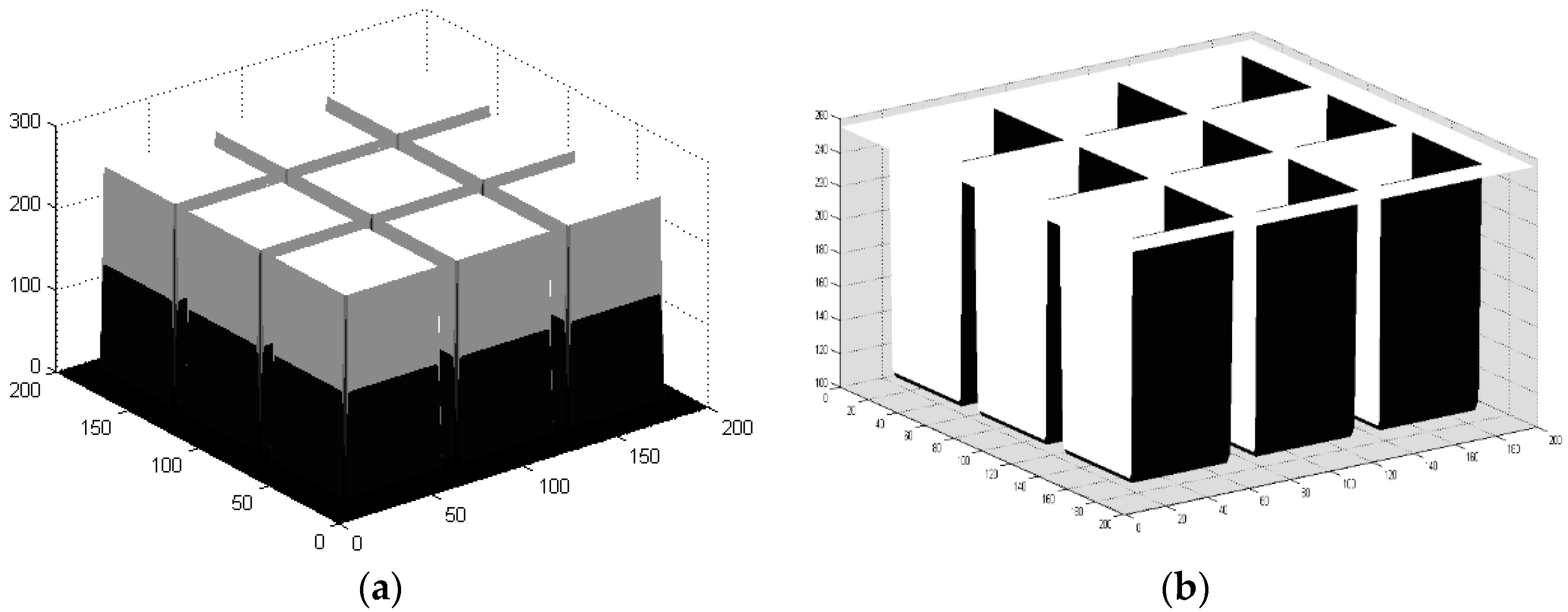
Figure 3. In addition, we also calculated the corresponding image data fields, as shown in
Figure 4.
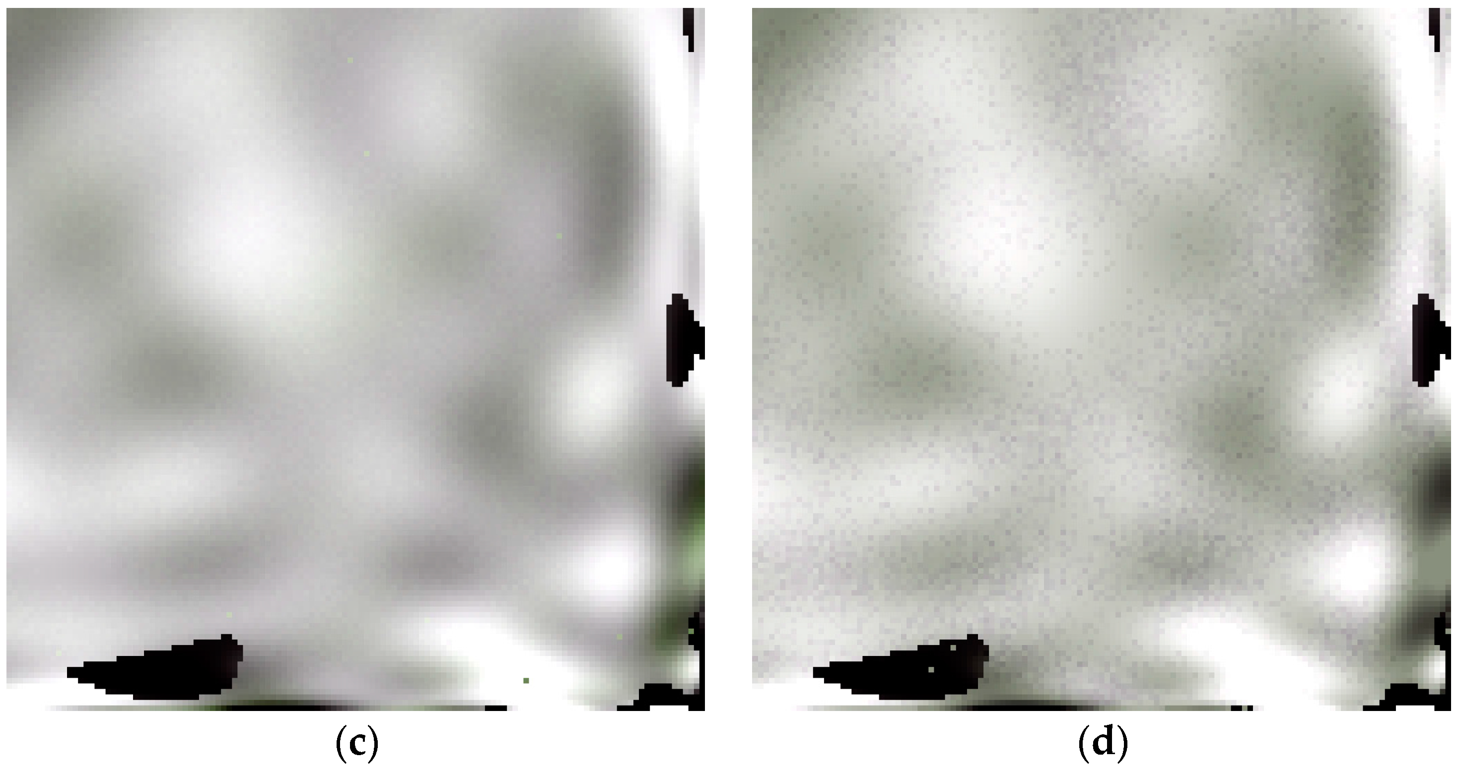
When the centre pixel and the neighbouring pixels of the homogeneous region are relatively high values, they are called the high grey value areas (the nine patches in
Figure 3a). Conversely, the homogeneous regions containing low-value pixels are called the low grey value areas (the nine patches in
Figure 3b). The data field calculated from the above figure shows that the average potential energy of the high grey areas is also high, so there exists a maximum in the local data field space. In contrast, the potential value of the nine patches is significantly lower than that of the edge region with a higher background value. In addition, both high-value areas and low-value areas are defined as homogeneous regions [
24,
25]. The normal endmember in the image space we are examining may exist in the geometric centre of a homogeneous region, corresponding to the potential extreme values of the data field space. Therefore, using the data field theory to locate the endmembers corresponds to locating the maximal or minimal points in the data field where the “potential cores” of the homogeneous area are located. The normal candidate endmembers are always located in the “potential cores” of the data field.
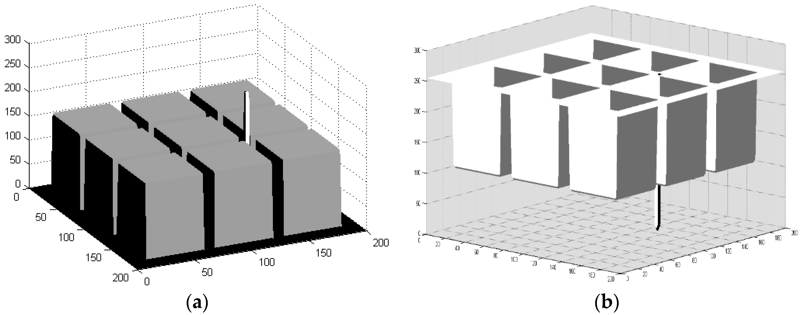
To explore the performance of the anomalous endmember extraction using the data field theory, anomalous pixels were added to the above simulated images. The corresponding data fields were then calculated, as shown in
Figure 5 and
Figure 6.
The accuracy of the anomalous endmember extraction directly affects the accuracy of the spectral unmixing. It is shown in the above figures that when an anomalous pixel is added to a corner of a simulated image, the anomalous pixel will form an obvious extreme in a neighbouring range of the local data field. On the other hand, the endmember of the homogeneous region will also generate many extreme points in the data field space. Therefore, to extract the extreme in two places, that is, to extract the local potential cores of the image, we can extract the candidate endmembers, including the anomalous endmembers and the homogeneous endmembers. This procedure lays a theoretical foundation for extracting candidate endmembers using data field theory.
In this step, in the process of the data field index calculation, with the help of principal component analysis (PCA) [
26], we used the first three principal components of the hyperspectral image and the impact factor σ as the inputs and obtained a set of data field values derived from the input image as the outputs.
2.4. Fusion of Data Field and Spectral Information
This step takes the data field pixels calculated in step 1 and the spectrally purest pixels identified in step 3 as the inputs. The two index results were calculated by means of a dot product computation, carried out point by point.
Finally, it returned a subset of pixels from the original hyperspectral image, which were preprocessed to subsequently extract the endmembers.
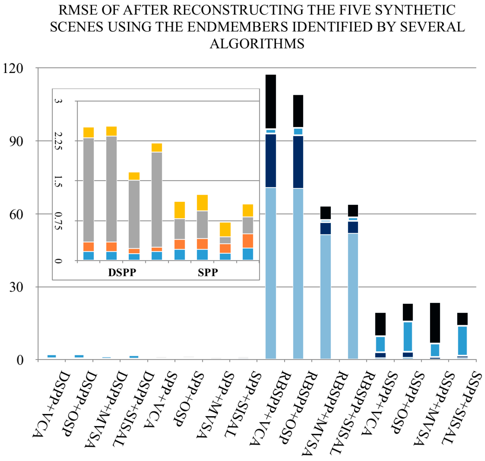
Moreover, in addition to using the DSPP endmember preprocessing algorithms for endmember candidate extraction, we also used OSP, VCA, MVSA, and SISAL to extract the exact endmembers. The reasons why we selected these extraction algorithms are as follows: (1) They are fully automated; (2) They require no additional input parameters other than the endmember number
e; (3) The four algorithms can be divided into two groups. OSP and VCA are based on the pure signature assumption, whereas MVSA and SISAL are considered minimum volume methods. Therefore, the latter two algorithms do not assume that the endmembers exist in the image. At last, we applied a fully constrained linear model [
28] to complete the hyperspectral unmixing. The result of this process is a set of
e endmembers and their corresponding abundance estimation maps.


