4.1. LC/LU Maps
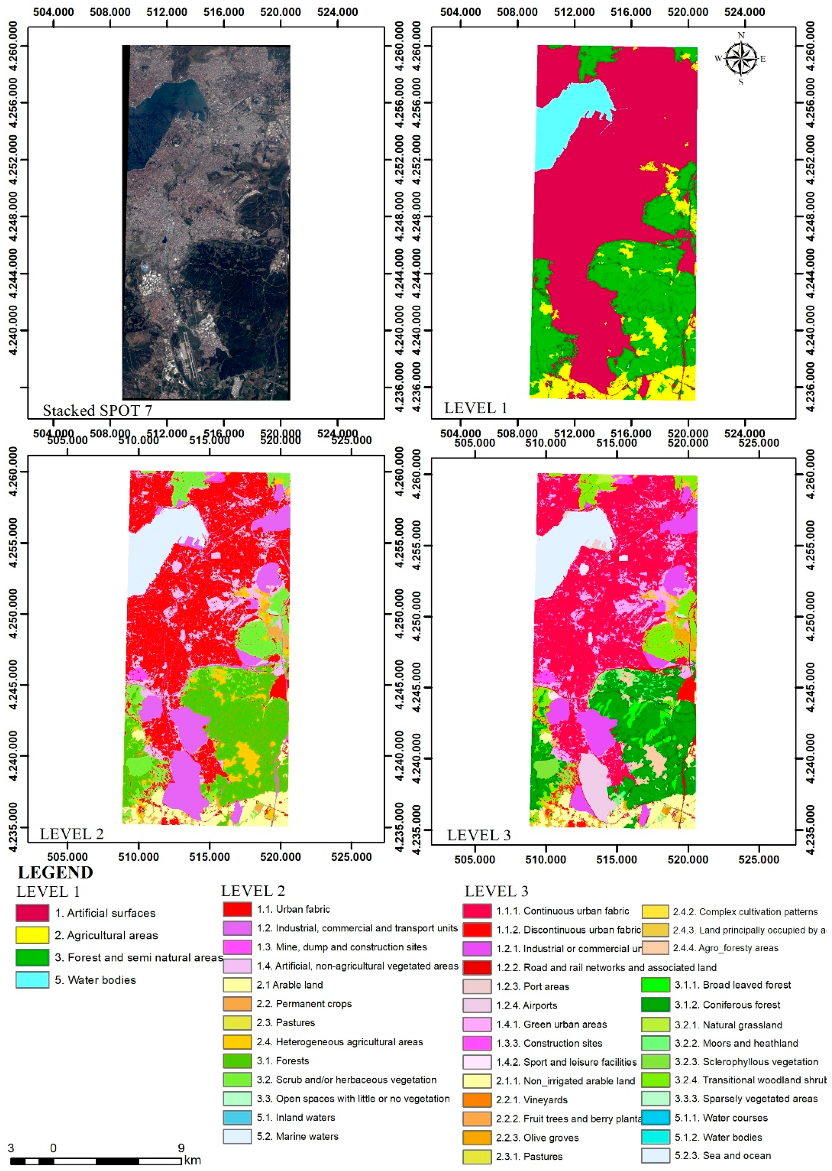
In this study, 3 different levels of LC/LU maps were produced according to CORINE nomenclature by applying GEOBIA technique on multi-temporal SPOT 7 images.
Figure 4 illustrates the classification results. In the map of Level 1, Artificial Surfaces (1) cover 167 km
2, Agricultural Areas (2) cover 25 km
2, Forest and Semi-Natural Areas (3) cover 73 km
2, and Water Bodies (5) cover 18 km
2 area. According to classification results, Artificial Surfaces is the dominant land cover type within the study area. A variety of artificial classes could be deducted from Level 2 and Level 3 classifications with more thematic details. As an example for Artificial Surfaces, 4 and 9 different artificial sub-classes were obtained in Level 2 and Level 3, respectively for the study area. These thematic details could provide efficient and precise information on urban, transport, industrial, port areas that could be used as an input for variety of different applications ranging from landscape architecture to environmental studies. Semi-Natural Areas (3) also cover a large proportion when compared to other classes. Evaluation of the generated maps showed that class diversity is quite significant especially at the Level 3 LC/LU map. This suggests the difficulty of keeping the accuracy high during the classification process. In addition, the SPOT 7 image was not enough by itself to determine some LC/LU classes of Level 3 LC/LU map, such as Industrial or Commercial Units (121), and Olive groves (223). Inclusion of different thematic layers shown in
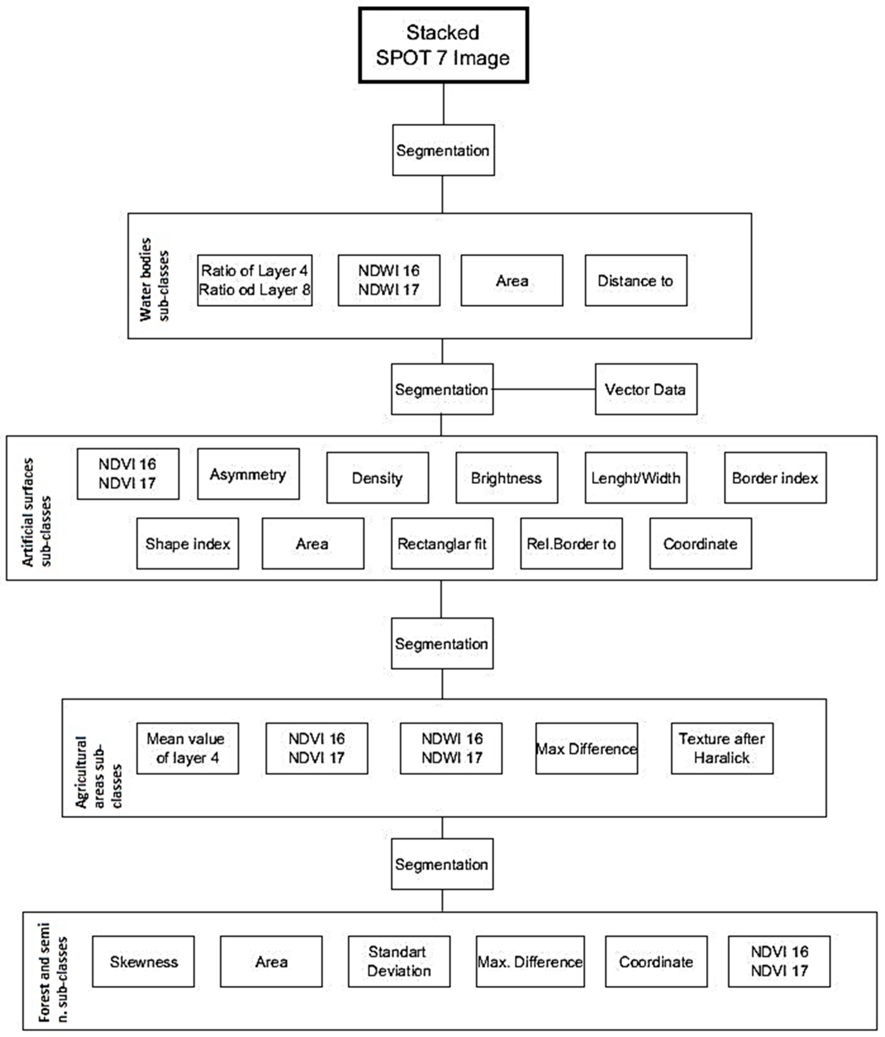
Table 3 into the classification improved the results. Considering the different number of patches and classes in different levels, landscape metrics of three different levels provided various information.
Selection of the most appropriate LC/LU classification system is an important step and there are different standardized nomenclatures available for this purpose. For most of the LC/LU systems, hierarchical levels are available in which the 1st Level represents general land cover classes and thematic detail, and complexity in class definition increases in 2nd and 3rd Levels. We used 3 Level hierarchical CORINE-based classes in this research. Although generating 1st Level classes such as Artificial Surfaces, Agricultural Areas, Forest and Semi-natural, Water Bodies are easy and could be automatically done by object based classification approaches in conjunction with some spectral indices, classification of Level 2 and Level 3 thematic classes is a more challenging task to automatize. Specifically, for some Level 3 Artificial Surfaces classes, land use information is crucial, which could not be directly produced from satellite images. In such cases, integration of open source geo-information to segmentation and classification stage improved the accuracy of classifications and lead to identify thematically detailed LC/LU classes. It is important to use multi-temporal data from different seasons to accurately identify agriculture and vegetation related 2nd and 3rd level classes such as Broad-Leaved Forest, Coniferous Forest, Non-irrigated Arable Land and Permanent Crops. Texture based Haralick features are used as an important indicator for the identification of some permanent crops such as Vineyards.
4.3. Landscape Metrics
Landscape metrics such as Number of Patch (NP), Edge Density (ED), Largest Patch Index (LPI), Euclidean Nearest Neighbor Distance (ENN), Splitting Index (SPLIT) and Aggregation Index (AI) metrics are useful indicators to assess the landscape configuration of related regions by using satellite based LC/LU maps. Landscape metric values change with classification levels; therefore, it is important to select the most appropriate classification level for a given area. Most of the studies conducted in the literature are based on Level 1 LC/LU class metrics, which could only provide very general information about the related region. Calculation of landscape metrics for Level 2 and Level 3 classification scheme leads to better understanding of the configuration and composition of the landscape.
Table 9,
Table 10 and
Table 11 provide the class-level metric calculation results for each of the three different levels LC/LU maps.
Calculated metric values according to Level 1 classification show that Artificial Surfaces (1) is the dominant class in the study area (PLAND = 56.45). Although the NP value of the Artificial Surfaces (1) class is lower than the NP value of the Forest and semi-natural areas (3) class, the LPI, ED, TCA values are higher than the other classes. These values show that compact and related patches are concentrated on this class. ENN_AM, weighted with respect to the patch size, refers to the neighborhood relations of the patches in terms of proximity. According to this metric value, patches that belong to Artificial Surfaces (1) are in a close relation to each other. Also, SPLIT shows that the scattering in Artificial Surfaces (1) is low. Water bodies (5) was identified as the most passive class in terms of PD, NP and PLAND. Patches are too small and too far from each other to develop an edge-core relationship. This relationship is important as it presents the ability of a patch to interpret stability or change in time and it increases the meaning of shape metrics.
Even though it covers half of the surface compared to Artificial Surfaces (1) class, NP and PD values of the Forest and Semi-Natural Areas class (3) are quite high. When considered with the low level of LPI (6.68), these results suggest that this class is undergoing fragmentation over time. It can be also asserted that the Forest and Semi-Natural Areas (3) class, which has the highest LSI value, has a complex structure and formed by natural geometries with relatively natural lines with natural geometries form it. However, in terms of ED and TCA values, it is behind the Artificial Surfaces (1) class. In particular, TCA value is significantly lower (4039.79) when compared to Artificial Surfaces (15,050.68). This shows that patches of Forest and Semi-Natural Areas class (3), have started to lose their core properties and edge relations have been weakened.
Agricultural Areas class (2) was identified as the class with the highest class fragmentation in Level 1. Although value of NP is much higher compared to class Water Bodies (5), which covers the smallest surface in the study area, Agricultural Areas class (2) has the lowest LPI value (1.39). It also has the lowest value for TCA. These values show that the patches in Agricultural Areas (2) are small, undeveloped and according to the values of SPLIT and ENN_AM they are scattered and not connected.
Water bodies class (5), which covers the smallest area in the study region and also is the weakest class in terms of NP and PD has the closest LSI value (3.27) to the geometric form. ED values of patches that belong to this class were found to be particularly low (1.89). Patches are relatively far apart (ENN_AM = 24.96) and scattering level is very high (SPLIT = 266.54) though not as much as the Agricultural Areas class (2).
All of these evaluations of Level 1 class metrics show that, the patches of the Artificial Surfaces (1) in the landscape are compact, big, interrelated and they have mature edge-core relationships. Results conclude that Artificial Surfaces (1) dominate the landscape. Agricultural Areas (2) are scattered in the region as disjointed small units. Forests and Semi-Natural Areas (3) are suppressed by Artificial Surfaces (1) both in area and patch relation. Water Bodies (5) is the weakest class in terms of area, patch density and patch number. Geometry of the water surfaces in the area exhibits unnatural, geometrical forms. These results indicate that water sources in the area are insufficient in terms of ecology.
Analysis of Level 2 and Level 3 class metrics show that Urban Fabric (11) and Continuous Urban Fabric (111) classes are dominant classes at their respective levels.
At Level 2, Urban Fabric (11) which is dominant in terms of NP, PD, PLAND and ED metrics, is behind Industrial, Commercial, and Transport Unit (12) class in terms of TCA, LSI and LPI metrics. In terms of patch and percentage of landscape Urban Fabric (11), in terms of shape and dominant patch class Commercial, and Transport Unit (12) classes stand out. It had been determined that, the dominant class among the Agricultural Areas classes (21, 22, 23 and 24) is Arable Land (21). The values of PLAND, PD, NP and LPI metrics of this class are relatively higher. Heterogeneous Agricultural Areas (24) and Permanent Crops (22) are the classes that enables the general Agricultural Areas of Level 1 to have a heterogeneous form because of their high LSI values. On the other hand, the most disjointed sub-category in terms of the distance between the patches is Permanent Crops (22), while SPLIT shows that the most scattered is Pastures (23).
Assessment of Level 3 metric results shows that, classes that dominate Level 3 in terms of PLAND and LPI are forest classes (311, 312 …, 333). Forest classes are in large units (LPI = 4.79) with centralized area development (TCA = 2397.37). Coniferous Forest (312) leads the forest classes in terms of both PLAND and LPI, and it also has developed edge-core relations (TCA and ED). Transitional Woodland Shrub (324) has the highest patch values (PLAND, PD, NP and LPI). LSI metric of class Moors and Heathland (322) shows that it is the most natural class among others. The interpretation that applies to the whole forest classes at Level 3 is, they have the largest fragmentation (SPLIT = 157,027.38) and the longest average distance between patches (ENN_AM = 18.37). Another notable class at Level 3 is the Olive Grooves class (223), which increases overall LSI value of Permanent Crops. These results revealed that, this class is in a more heterogeneous form than the other sub classes of Permanent Crops.
An overall evaluation of Level 2 and Level 3 metrics shows that, according to PLAND, NP and PD metrics, Level 3 class Continuous Urban Fabric (111) induce the Level 2 class Urban Fabric (11) which means class 111 increases the metric values of class 11. Similarly, Road and Rail Networks and Associated Land class (122) induce Shape Metrics and LPI of Industrial, Commercial and Transport class (12).
It is interesting that the class which causes the patch shape to be more indented (LSI = 600.10) is essentially a linear class. This can be explained by the fact that the Urban Fabric (11) class has a much higher SPLIT ratio than Industrial, Commercial and Transport units (12) classes. A large number of patches of class Urban Fabric (11) are scattered throughout landscape, while class Industrial, Commercial and Transport class (12), which has the lowest SPLIT ratio (57.91), forming more complete and uniform patches (LPI = 13.14) which means that shape irregularities and patch shape has become more heterogeneous. On the other hand, Construction Sites class (131) induces the fragmentation (SPLIT) of class Mine, Dump and Construction Sites class (13) in Level 2. In this class, which stands out with a very low PLAND (0.54), a few patches (NP = 8) are located far away from each other and scattered within the landscape.
Discussion of spatial metrics and their possible contribution to landscape ecology should also address the issue of what these measures are to be compared against [
54]. The findings of this research showed that selected metric sets are successful for revealing landscape characteristics at different levels of classification. Using detailed class definitions while keeping the scale level constant, enabled a more comprehensive interpretation of landscape characteristics. Additionally, performing these observations based on quantitative data is a valuable contribution for landscape analysis and evaluation.

 ,
, 


