An Algorithm based on the Weighted Network Voronoi Diagram for Point Cluster Simplification

Abstract

Points on maps that stand for geographic objects such as settlements are generally connected by road networks. However, in the existing algorithms for point cluster simplification, points are usually viewed as discrete objects or their distances are considered in Euclidean spaces, and therefore the point cluster generalization results obtained by these algorithms are sometimes unreasonable. To take roads into consideration so that point clusters can be simplified in appropriate ways, the network Voronoi diagram is used and a new algorithm is proposed in this paper. First, the weighted network Voronoi diagram is constructed taking into account the weights of the points and the properties of the related road segments. Second, the network Voronoi polygons are generated and two factors (i.e., the area of the network Voronoi polygon and the total length of the dilated road segments in the polygon) are considered as the basis for point simplification. Last, a Cartesian coordinate system is built based on the two factors and the point clusters are simplified by means of the “concentric quadrants”. Our experiments show that the algorithm can effectively and correctly transmit types of information in the process of point cluster simplification, and the results are more reasonable than that generated by the ordinary Voronoi-based algorithm and the weighted Voronoi-based algorithm.

1. Introduction

Point clusters are widely used to visually represent geographic features on maps. For example, settlements, islands, and control points can be presented using point symbols on certain scale maps [1]. When the scale of a map containing point symbols becomes smaller, the point clusters generally become crowded and the map becomes illegible. Under such a circumstance, the point clusters need to be simplified so that the smaller scale map can be read easily. In the process of point cluster simplification, some more important points are retained and the other less important ones are deleted. Automated simplification of point clusters depends on algorithms. By far many achievements have been made at this aspect. As shown in

Table 1. Two types of algorithms for point cluster simplification.

Algorithm	Weights	Values of the Weights
Settlement-spacing ratio-based	Yes	Given based on the importance of the settlements
Gravity modeling-based	Yes	Given based on the importance of the settlements
Distribution-coefficient	Yes	Given based on the importance of the settlements
Circle-growth	Yes	Given based on the characteristics of the points
MWVD-based	Yes	Given according to experience of experts
Hierarchical Voronoi-based	Yes	The distance between the current point and other points
Convex hull-based	No	/
On spatial distribution properties preservation	No	/
Genetic Algorithm	No	/
Dot maps simplification	No	/
Circle characters-based	No	/
Kohonen-based	No	/
Ordinary Voronoi-based	No	/

Note: ‘/’ means the algorithm does not take the weights into account.

, existing algorithms can be divided into two categories: the ones that consider weights and the other ones that do not.

The first type includes five algorithms. Three of them are proposed by Langran & Poiker (1986), i.e., the settlement-spacing ratio algorithm, the distribution-coefficient algorithm and the gravity model. In these algorithms, the simplification is done based on the importance of the settlements and the two-dimensional Euclidean distances between settlements [2]. In addition, van Kreveld et al. (1995) proposed an algorithm based on the idea of circle growth, in which the weights of the points were represented as the size of circles, and the simplification is done based on the size of corresponding circles [3]. The fourth one, the algorithm based on a multiplicatively weighted Voronoi diagram (Yan & Wang, 2013), sets the weights of the points according to the experience of experts, and the weighted Voronoi diagram is employed in point cluster simplification [4]. The last one is proposed by Li et al. (2014), which is based on the hierarchical Voronoi diagram. In the algorithm, the cluster analysis and simplification are done based on the linear distance between current point and other points [5].

The second type includes seven algorithms. The first one is the algorithm based on the convex hull (Wu, 1997), it simplifies point clusters by merging the convex hulls and simplifying the polygons. It can transmit the distribution characteristics of the original point cluster well [6]. The second one is the algorithm for spatial distribution properties preservation (Ai & Liu, 2002), which simplifies the outer points and the internal points respectively to maintain the geometric characteristics of the point cluster [7]. The third one is the algorithm based on the genetic algorithm (Deng et al., 2003). It simplifies point clusters by the adaptive algorithm and the generic algorithm, and it can transmit the distribution scope and local density well [8]. The fourth is the dot map simplification algorithm (de Berg et al., 2004), which simplifies points by ε-approximation and clustering algorithms, and the distribution density and clustering characteristics of the original point cluster can be maintained well through the simplification [9]. The fifth algorithm is based on circle characters (Qian et al., 2006), which simplifies point clusters by repetitive clustering and simplifying operations. It can maintain the distribution center and scope correctly after simplification [10]. The sixth one, a Kohonen net-based algorithm (Cai et al., 2007), can well and effectively preserve the local density and structure characteristics of the original point clusters [11], and the last one, a Voronoi diagram-based algorithm (Yan et al., 2008) can maintain the geometric and topological features after point cluster simplification [12].

It can be concluded that the second type of algorithm focuses on the preservation of geometric structure and topological features of the original point clusters in the simplification. Nevertheless, the weight of the point is ignored in this type of algorithm. In the first type of algorithm, although the weight of the point is considered in the simplification, two problems still exist:

(1) The world is abstracted as an infinitely homogeneous and isotropic space, and the distance between two events or facilities is measured by the Euclidean distance [13,14]. However, in the real geographic space, the connection or the distance between points is usually constrained by the road network.

(2) Road networks are not taken into account in these algorithms, which can generate the same results if the same point cluster is put into two different road networks and simplified by the same algorithm. This is obviously unreasonable, because the relations among the points are not pure geometric relations but are affected by the road network [15].

To settle down the two problems, the “network Voronoi diagram” is introduced into the new algorithm. It is a type of special Voronoi diagram which establishes links between facilities by considering the road network related to the facilities rather than only the Euclidean distances among them. To be specific, it takes into account the properties of the roads related to the facilities. Compared with the ordinary Voronoi diagram, the network Voronoi diagram is more appropriate for analyzing the spatial phenomena and activities that are constrained by networks. For example, it has been applied in analyzing traffic accidents and crime distribution and describing service regions [15,16,17,18]. Thus, it should be a natural thought to use network Voronoi diagrams to simplify the point clusters that stand for geographic entities on the Earth and are closely related to the nearby road networks.

The organization of this paper is as follows. After this introduction, the idea of the new algorithm is introduced in Section 2. The construction of a weighted network Voronoi diagram (Section 3) and the generation of network Voronoi polygon (Section 4) are presented in detail; the procedure of the deletion of the point is illustrated in Section 5, and then the experiments will be illustrated and discussed to test the validity of the new algorithm (Section 6). Finally, some conclusions will be drawn and a number of potential research topics will be given (Section 7).

2. Framework of the New Algorithm

Suppose that a number of settlements in a block of a city are represented as point cluster on a map at scale S, and the information of the roads pass through the block is given (Figure 1). If the scale of the map becomes S/5, the points on the map become crowded and need to be simplified. Figure 2 shows the procedure of the point cluster simplification proposed in the new algorithm.

This network Voronoi diagram-based algorithm comprises three steps: (1) Firstly, the weighted network Voronoi diagram is constructed by taking into account the grades of the points, the traffic capacity, and the directions of the related road segments. After that, the different roads are distributed to different points (marked in different color in Figure 3b). (2) Then, the network Voronoi polygons are constructed (Figure 3c), where the area of the network Voronoi polygon and the total length of dilated road segments in the polygon are proposed and used to calculated the selection probability of the points. (3) Lastly, the point deletion is carried out based on the selection probability of the points.

3. Construction of Weighted Network Voronoi Diagrams

To construct weighted network Voronoi diagrams, the stream flowing method, which has been tested to be an effective method for constructing the network Voronoi diagrams, is employed here [18]. It is described step by step in the following subsections.

3.1. Network Tessellation

The roads are tessellated to obtain a discrete representation, which is similar to the rasterization of the planar space. This can be achieved by the following way: First, the road network is broken into a set of consecutive segments connecting two neighboring road intersections (e.g., AB and BC in Figure 4). Second, each segment is subdivided into a number of equal-length linear units, which are referred to as lixels. The lixels can be interpreted as the line pixel in an image [19]. It should be noted that the length of the linear unit is set according to the practical application. For example, compared with the bus stop, the service region of a train station is much greater and a greater lixel length can be set for the network tessellation.

Once the road network is tessellated, points are projected onto the nearest lixels. The thick linear units in Figure 4 represent the projected lixels.

According to the role the lixels play in the dilation operation, the lixels may be classified into three types: (1) unoccupied lixel, (2) expanding lixel, and (3) occupied lixel. An unoccupied lixel refers to the one that has not been occupied by any of the generators (e.g., S₁ in Figure 4). An expanding lixel is the one that has been occupied by a generator but has at least one unoccupied neighboring lixel. It acts as an active head in dilation operation (e.g., S₂, S₄ in Figure 4). An occupied lixel refers to the one itself and its neighbors have been occupied (e.g., S₃ in Figure 4).

3.2. Expansion Operator

The idea of stream flowing which is similar to the expansion principle in mathematical morphology is employed in expansion operations here [18]. In the process of expansion, the projected lixels of the points are viewed as the source of the generator starting from which the flows expand with a certain step along with related road segments simultaneously. The flows expand along different tributaries before they reach the intersections of the road network, and the expansion does not stop until the flows encounter each other or reach the end of the road network (Figure 5). As a result, the routes taken by different generators form the network Voronoi diagrams, which partition the impacting area in the network space.

As shown in Figure 5, the stream flowing assumes that the streets are two-way and in homogeneous spaces, and the facility features have equal importance. However, in the real geographic world, some roads are one-way and/or less important, and some others might be two-way and/or more important, and the point features themselves have different importance. Obviously, all of the factors take effect in computing the influential regions of the facilities. Therefore, these factors should be considered when the expansion speed is calculated. These factors are listed as follows:

• Direction of the roads

The flow can expand along the road if its expanding direction is the same as the direction of the road. Otherwise, the flow cannot expand along the road, e.g., if the road extends from west to east, the flow that is expanding from east to west has to stop on this road. This can be expressed by Equation (1):

$$L_{p1}=k\times F(P_1,P_2)$$

(1)

where, L_P1 is the expansion unit, k is the standard length of a lixel, and F(P₁, P₂) is a direction function. If the flow is the same as the direction of the road, F equals 1; otherwise, F equals 0.

• Traffic capacity of the roads

Because different categories of roads have different traffic capacity, the new algorithm set different weights for different categories of roads, e.g., assign 2 to arterial roads and 1 to secondary roads. The function that traffic capacity plays in the expansion operation can be expressed by:

$$L_{p2}=k\times W(x)$$

(2)

where, L_P2 is the expansion unit and W(x) denotes the traffic capacity of the roads.

• Weight of the points

The weight of the point depends on the scale and power of the corresponding facility. The higher the weight of the point, the larger its influence area is, which can be represented in expansion operation by Equation (3):

$$L_{p3}=k\times W(p)$$

(3)

where, L_P3 is the expansion unit and W(p) denotes the weight of the point.

If all the above factors are considered, the expansion speed can be defined as Equation (4)

$$L_p=k\times W(x)\times W(p)\times F(P_1,P_2)$$

(4)

Figure 6 shows the expansion result when all of the three factors are considered, where routes that are generated from different points are marked in different colors.

4. Construction of Network Voronoi Polygons

In the weighted network Voronoi diagram, the road network and its related space are assigned to different points. The road segments generated from the same point (marked in the same color in Figure 6) may constitute a polygon region. The polygon region which can be named network Voronoi polygon can represent: (1) the importance of the point, which is the basis of the point simplification; and (2) the distribution characteristics of the point cluster, which should be considered in the simplification of the point cluster. Therefore, the network Voronoi polygon is important in the simplification of a point cluster. Its construction is described as follows:

Step 1: Construct the constrained Delaunay triangulation using the nodes of the road segments (points P₁-P₁₂ in Figure 7a) [20].

Step 2: Calculate the boundary polygon by the method of dynamic threshold ‘stripping’, which may be described below:

(1) Set threshold $d=k\times Avelength$, where k is the grade of ‘stripping’ (here, k = 2) [21], Avelength is the average value of all the triangle edges in the Delaunay triangulation, and d is dynamically updated after every “stripping” [22].

(2) Compare every outside non-feature edge (the edge which has only one adjacent triangle and is not the feature edge of the linear object group) with threshold d. If it is greater than d, then determine if the other two edges of the current triangle can form a triangle with any other edge after deleting the current edge. If the result is positive, delete this edge and turn to 3), otherwise the edge should be retained; repeat this step.

(3) Set the other two edges of the triangle that the deleted edge belongs to as outside edges, recalculate the value of Avelength and update the value of d. Strip inward layer by layer until the length of all the outside non-feature edges is less than the current threshold d.

The ‘stripping’ result of the linear object group in Figure 7c is shown in Figure 8a.

(4) Connect the outside edges end to end to form the final boundary polygon (Figure 8b).

By doing this, the network Voronoi polygons are constructed (i.e., S₁ in Figure 9), by which the weights of the points can be calculated and the point cluster simplification can be done.

5. Deletion of Points

5.1. Strategies Used in Information Transmission

One of the main goals of the algorithm for point cluster generalization is to correctly transmit the information contained in the original point cluster. Therefore, some strategies are used in the proposed algorithm to transmit the four different informations on point maps, i.e., statistical, thematic, topological, and metric information [23].

• Statistical information

The Radical Law is an extensively applied method for calculating the number of objects that should appear on a target scale map in map simplification. Thus, the number of points that should be retained on the target map can be determined by Equation (5) [24].

$$N=N_0\cdot \sqrt{S_o/S_f}$$

(5)

where, N is the number of points on the target map; N₀ is the number of points on the original map; S_o is the denominator of the original map scale, and S_f is the denominator of the target map scale.

• Thematic information

The importance of the point is considered as the basis for point cluster simplification, which is decided by both the weight of the point and the properties of the related road segments. In the new algorithm based on the weighted network Voronoi diagram, it can be seen that the weight of the point and the properties of the road segments can be represented by the network Voronoi polygons.

For the network Voronoi polygon, firstly, the region of it will be larger if the point and its related road segments are more important; secondly, it has a lot to do with the density of the road network. The resulting network Voronoi polygons can be quite different, although the flows expand with equal speed at equal times. For example, the network Voronoi polygon of P₁ is larger than that of P₂ (Figure 10), but the total length of the expanded routes (road segments in polygon) of P₁ is smaller than that of P₂. Such results were produced because of the different local densities. Thus, the regions of the network Voronoi polygons as well as the total length of dilated road segments in the polygon are treated as the basis for point simplification. In the following simplification, a basic rule is generally abided by: ‘the larger the network Voronoi polygon and the longer the total length of dilated road segments in the polygon, the more probable the point can be retained on the resulting map’. This rule obviously may ensure that the points of great importance and points next to the important roads have a higher possibility to be shown on the generalized map.

In the new algorithm, the relative area of the network Voronoi polygon (P_i1) and relative total length of road segments in polygons (P_i2) are computed by Equation (6) and Equation (7). After that, P_i1 and P_i2 together determine the probability of a point to be retained.

$$P_{i1}=A_i/{\displaystyle \sum _{i=1}^n{A}_i}$$

(6)

where, A_i is the area of the network Voronoi polygon of the i^th point.

$$P_{i2}=l_i/{\displaystyle \sum _{i=1}^n{l}_i}$$

(7)

where, l_i is the total length of road segments in the network Voronoi polygon of the i^th point.

There may be a special case in which the road segments generated from a point cannot form a polygon, e.g., there is only one road segment generated from the point. In this situation, only the length of the road segment is calculated for thematic information.

• Topological information

Although it is impossible to protect topological relations among the points in the process of point cluster simplification, it is still a principle to try and minimize damaging their topological relations. Thus, the rule ‘do not delete any two neighboring points’ needs to be observed [25], i.e., any two points whose network Voronoi polygons are neighbors cannot be deleted simultaneously in the same round of point deletion.

In the simplification, each point may be in one of the three statuses: ‘fixed’, ‘deleted’, or ‘free’. In the beginning, all the original points are marked as ‘free’. If a point is marked as ‘deleted’, it means that this point is a candidate that will be deleted but not all at once. To ensure the efficient transmission of the topological information, if a point is marked as ‘deleted’, its neighbors should be marked as ‘fixed’. Fixed points cannot be marked as ‘deleted’ in the same round of point deletion, ensuring that no adjacent points are deleted simultaneously. This step is repeated until no points can be marked as ‘deleted’. In this procedure, the points marked as ‘fixed’ belong to typeⅠ, which will be retained; the points which are marked as ‘deleted’ belong to type II and will be deleted; other points belong to type III and will compete to decide whether they will be retained or deleted [26].

• Metric information

In the new algorithm, the relative area of the network Voronoi polygon that reflects the local relative density is employed as a metric measure. It works together with the rule ‘do not delete any two neighboring points’ and ensures that the metric information can be clearly transmitted.

5.2. Process of Point Deletion

In the process of point deletion, it is easy to select the points of type II because if a point will be deleted in the simplification, it is very likely that its relative area of the network Voronoi polygon (P_i1) and the relative total length of dilated road segments in the polygon (P_i2) are both small. If the corresponding points are marked in the Cartesian coordinate system, where the area of the network Voronoi polygon is the abscissa and the total length of the road segments in the polygon is the ordinate, the points of type II will be nearer to the origin of the system. Based on this, the point deletion is done as follows:

Step 1: The number of points to be deleted is determined by Equation (8):

$$n=\mathit{int}(N_0-N)$$

(8)

where, n is the number of points to be deleted; N₀ is the number of points on the original map, and N is the number of points on the target map which is calculated by the Radical Law.

Step 2: The values of P_i1 and P_i2 are marked as weighted points in the Cartesian coordinate system with P_i1 as its abscissa and P_i2 as its ordinate. The weighted points of the point cluster in the example are shown in Figure 11a.

Step 3: Concentric quadrants are drawn starting from a quadrant whose center is the origin and the radius is the distance between the origin and the nearest weighted point to the origin.

Step 4: Concentric quadrants are drawn recurrently at one step intervals of the minimum distance between the weighted points (Figure 11b). The weighted points on the current quadrant and in the stripe between it and the prior quadrants will be selected after each round, and their corrsponding points in the point cluster, whose statuses are ‘free’ and their neighbor points have not been marked as ‘deleted’, will be marked as ‘deleted’. Meanwhile, their neighbor points will be marked as ‘fixed’. After this round of marking, the number of points marked as ‘deleted’ will be compared with value n. If it is smaller than n, then Step 4 will be repeated; if it is greater than n, turn to Step 5; otherwise, turn to Step 6.

Step 5: The points that have been marked as ‘deleted’ in the prior stripe are marked as “free” and they will compete with each other to decide which one should be deleted. The area of the network Voronoi polygon is treated as the main basis for deletion in this situation. The corresponding points are sorted by ascending order of the area of their network Voronoi polygons, and the points in the tail will be marked as ‘deleted’. Turn to Step 6 until the number of the points marked as ‘deleted’ equals n.

Step 6: The points marked as ‘deleted’ are deleted from the point cluster and the rest points constitute the target point cluster.

6. Experimental Studies and Discussion

6.1. Experiments

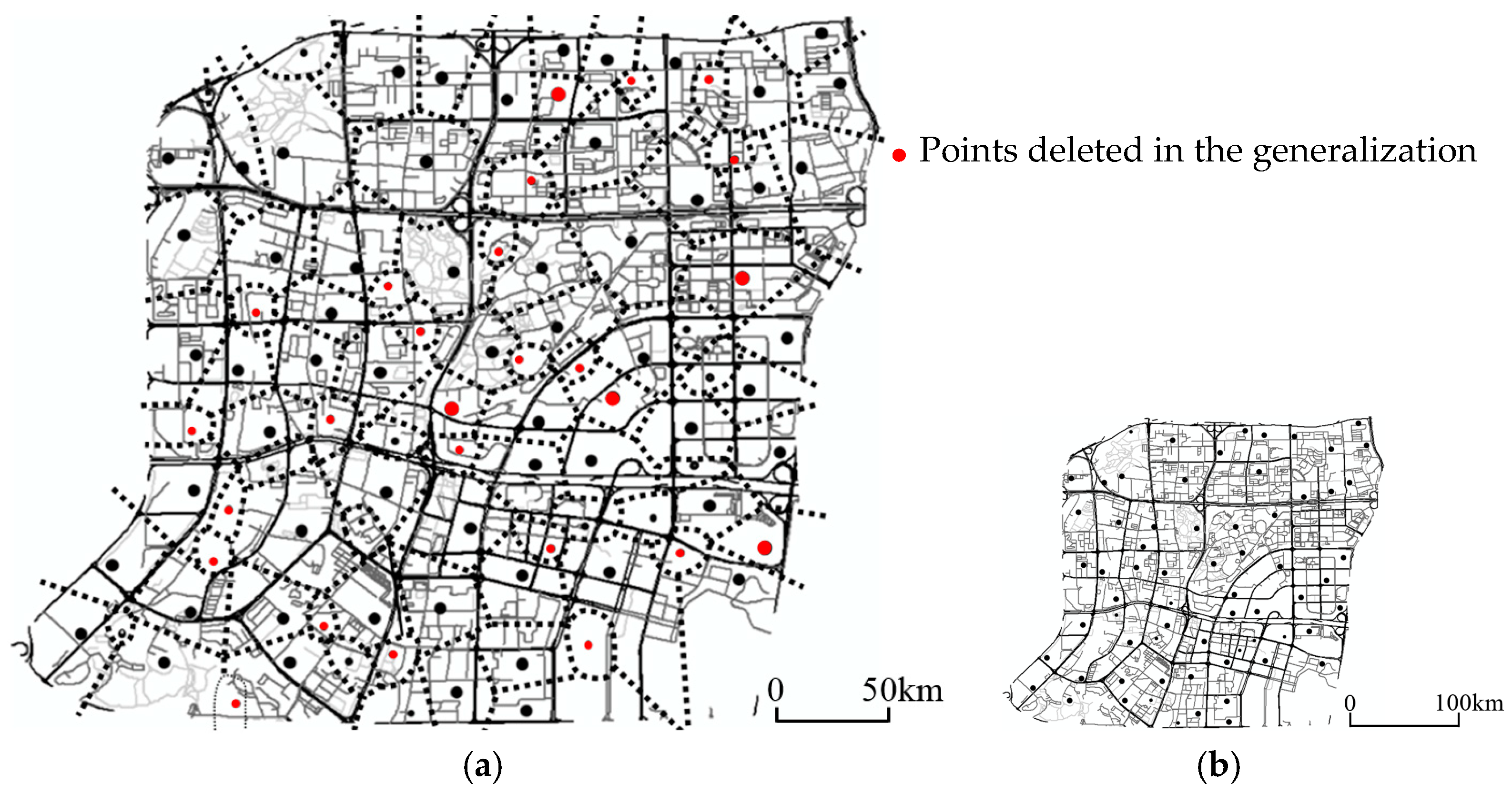
The new algorithm has been implemented by the authors in Matlab (R2013a) on Microsoft Windows 7. A number of datasets have been used to test the validity of the algorithm, and two of them are shown here. The data used in experiment 1 is a block of the Lanzhou City, China which contains 10 hospitals and 337 road segments, as shown in Figure 12a. The hospitals are of the same weight, and the road segments are of the same category. The original map scale is 1:10K and the target map scale is 1:25K. The dataset used in experiment 2 shows a much more complicated city block (it is Shenzhen city, China) compared with that in experiment 1. This map contains 96 educational institutions (63 public educational institutions and 33 private educational institutions) and 4652 road segments (2217 arterial road segments, 1765 secondary road segments, and 670 pedestrian road segments), as shown in Figure 13a. The original map scale is 1:50K and the target map scale is 1:100K.

To demonstrate that the results generated by the new algorithm are more reasonable than the algorithm based on the ordinary Voronoi diagram, the same point clusters shown in Figure 12a and Figure 13a are used to test them. The generalized results are shown in Figure 14b and Figure 15b, respectively.

It can be concluded from Figure 12 and Figure 14: (1) In Figure 12b, the flows generated from different points are of the same expansion speed, because all points have the same weight and so do the roads. (2) In the simplification based on the proposed algorithm, the effect of the road network on the influence region of the points is taken into account. For example, it can be seen that P₉ is deleted and P₈ is retained in Figure 12c, while P₉ is retained and P₈ is deleted in Figure 14b. This is because in the new proposed algorithm, P₈ has a larger influence region because it is nearer to the intersection of the road network than P₉ is. But in the algorithm based on the ordinary Voronoi diagram, P₈ is deleted because of a smaller Voronoi polygon than that of P₉.

The points marked in red in Figure 13b and Figure 15a are the points to be deleted in the process of simplification. From Figure 13 and Figure 15, it can be concluded that: (1) The points of greater importance have higher possibilities to be retained in the process of simplification if the data is generalized by the new algorithm (91.9% public educational institution are retained and 32.3% of private educational institutions are retained); (2) the points nearer to the intersections of roads are more likely to be retained in the simplification than the farther ones if the data is generalized by the new algorithm (i.e., P₁^’, P₂^’ in Figure 13c); (3) the points whose related roads have greater weights have greater possibilities to be retained after generalization if the data is generalized by the proposed algorithm (for example, P₃^’ in Figure 13c).

6.2. Algorithm Evaluation

As mentioned in the previous sections, the generalization algorithm should transmit the four types of information well. Therefore, the following standards are defined to evaluate the new algorithm quantitatively:

(1) The transmission rate of the statistical information (D_s) is measured by the deviation between the number of generalized points (N_g) and the theoretical number of points (N_o) that should be retained (Formula (9)).

$$D_s^{}=|N_g-N_o|$$

(9)

The smaller the value of D_s, the better is the transmitted statistical information.

(2) The transmission rate of the thematic information (D_th) is measured by the deviation between the average weight value of the original points ($\overline{W_o}$) and that of the generalized points ($\overline{W_g}$) (Equation (10)).

$$D_{th}=\overline{W_g}-\overline{W_0}$$

(10)

The greater D_th is, the more probable it is that points with greater weights are retained. Therefore, the greater D_th is, the better the thematic information is transmitted.

(3) The transmission rate of the topological information (D_tp) is measured by the difference between the mean number of the neighbors of the original network Voronoi polygon of the points on the generalized map ($\overline{d_g}$) and that of the original map ($\overline{d_o}$) (Equation (11)).

$$D_{tp}=\overline{d_0}-\overline{d_g}$$

(11)

The smaller D_tp is, the better the topological information is transmitted.

(4) The transmission rate of the thematic information (D_m) is measured by the change of the area of the range polygon (D_m), which can be evaluated by Equation (12).

$$D_m^{}=|\frac{P_o-P_g}{P_o}|$$

(12)

where, P_o is the area of the original range polygon, and P_g is the area of the range polygon on the generalized map.

The smaller D_m is, the better the metric information is transmitted.

The results of the indices calculated using the experiments are listed in

Table 2. Used in the experiments for evaluating the new algorithm.

Experiment	Algorithm	Ds	Dth	Dtp	Dm
Experiment 1	Algorithm based on the ordinary Voronoi diagram	0.68	/	0.59	2.85%
	New algorithm based on the weighted network Voronoi diagram	0.68	/	0.34	0.628%
Experiment 2	Algorithm based on the weighted Voronoi diagram	1	0.056	1.563	1.324%
	New algorithm based on the weighted network Voronoi diagram	0.21	0.154	1.412	1.383%

.

Table 2 indicates that the new algorithm transmits the information of the original points correctly after simplification. A number of insights can be gained from Table 2: (1) The number of the points on the generalized map obtained using the proposed algorithm is approximately equal to the theoretical number of the points that should be retained. (2) The deviation in the mean normalized weights (D_th) increases during the simplification, which means the points with greater weights are retained and those with less weights are deleted. (3) The average change of the number of the neighbors (D_tp) is small, which means the topological relations are transmitted well. (4) The change of the range polygon (D_m) is not large, and the errors are acceptable.

6.3. Discussions

From the experiments and evaluation, it can be seen that: (1) The network Voronoi diagram is different from the ordinary Voronoi diagram. The space divided by the ordinary Voronoi diagrams occupies the entire planar area, while the space divided by the network Voronoi diagrams only covers the space occupied by the road network. In addition, the boundary of an ordinary Voronoi polygon is a smooth line, while the boundary of a network Voronoi polygon is rather jagged. It can be imaged that the ordinary Voronoi diagrams and the network Voronoi diagrams can be the same if the road network is dense enough; and (2) the network Voronoi diagram performed better than the ordinary Voronoi diagram in point cluster simplification because roads are taken into account which adds more necessary and useful information to the construction of the weighted network Voronoi diagrams and, therefore, makes the process of point cluster simplification reasonable.

Compared with the algorithm based on the ordinary Voronoi diagrams, the algorithm based on the weighted network Voronoi diagram has higher time complexity, because all road segments in the road network are traversed in the construction of weighted network Voronoi diagrams.

Table 3. Time costed in point simplification.

Experiments	Lixel Length (m)	Number of Lixels in the Road Network	Total Time (s)
Experiment 1 (Figure 12)	1	1323	14.3
	5	321	7.1
Experiment 2 (Figure 13)	1	32859	19.4
	5	7278	9.1

shows the time costs for the experiments with different datasets and different lixel unit lengths at 1m and 5m, respectively. From the table it can be seen that the smaller length of the lixel unit is, the longer the experiment time, and the time cost has approximately linear growth with the refining process of lixel length. Thus, the determination of lixel length is a key problem in the construction of the network Voronoi diagrams as well as in point simplification. In the new algorithm, the lixel unit length is given according to the following factors: (1) The average distance between points, i.e., the greater the average distance between the two points, the larger the linear unit can be; and (2) the influence region of the point, for example, the influence region of train stations is much greater than that of bus stops; when we construct the network Voronoi diagram for train stations, the lixel unit length can be set much greater.

7. Conclusions

Point cluster simplification is an important part of map generalization. It also plays an important role in spatial analysis and urban planning. Because points that stand for geographic objects are generally connected and constrained by road networks, the network Voronoi diagram rather than the ordinary Voronoi diagram is used in the new algorithm. In addition, the importance of the points are affected by their connected and/or nearby road networks; therefore, in this new algorithm, the weighted network Voronoi diagram is employed as a tool to simplify point clusters and it is constructed by taking into account the weight of the points and the properties of the related road segments. To complement the point deletion, the network Voronoi polygons are generated and two factors (area of network Voronoi polygon and total length of dilated road segments in the polygon) are proposed and used to calculate the probability of the point to be retained. Based on these two factors, point simplification is done by the method of “concentric circle”.

The classic method of point simplification is based on the ordinary Voronoi diagrams or the weighted Voronoi diagrams. Compared with them, the proposed new algorithm has the following advantages: (1) more effective transmission of information of the original point cluster and (2) more reasonable generalization results because of the integration of the road network information into point cluster simplification.

Some pieces of progress made in this study can also be used in other similar domains. For example, the network Voronoi diagram as well as the network Voronoi polygon (Peterson et al., 2017) [27] can be applied to other research. The method of “concentric circle” proposed for point deletion can be used in other similar studies. The algorithm can also be extended to lines and polygons simplification. However, the algorithm may be further improved by introducing other possible factors such as human traffic and traffic flow into the construction of a network Voronoi diagram. We will apply the algorithm and improve it in the future.

Compared with the other algorithms, the difference of time-consumption between the new algorithm and the other existing algorithms lies in the time spent in the construction of the network Voronoi diagram, which has approximately linear growth with the refining process of lixel length. In practical applications, the length of the lixel can be adjusted by the actual demand. For example, the length of lixel can be set as a small value if higher accuracy is required; on the other hand, a big value can be set to the length of lixel if a higher speed is demanded. To solve the problem of large amounts of data, the divide-and-conquer approach can be referred to, i.e., the construction of a weighted network Voronoi diagram and the simplification of a point cluster can be done based on a series of space slices.