Article

Variables Selection for Aboveground Biomass Estimations Using Satellite Data: A Comparison between Relative Importance Approach and Stepwise Akaike’s Information Criterion

by
Rita Libertad Adame-Campos
1,*,
Adrian Ghilardi
1,2,
Yan Gao
1,
Jaime Paneque-Gálvez
1 and
Jean-François Mas
1
1
Centro de Investigaciones en Geografía Ambiental, Universidad Nacional Autónoma de México, Antigua Carretera a Pátzcuaro 8701, Col. Ex-Hacienda de San José de La Huerta, Morelia C.P. 58190, Mexico
2
Laboratorio Nacional de Análisis y Síntesis Ecológica (LANASE), Escuela Nacional de Estudios Superiores, Antigua carretera a Pátzcuaro 8701, Col. Ex-Hacienda de San José de La Huerta, Morelia C.P. 58190, Mexico
*
Author to whom correspondence should be addressed.
ISPRS Int. J. Geo-Inf. 2019, 8(6), 245; https://doi.org/10.3390/ijgi8060245
Submission received: 19 February 2019 / Revised: 1 April 2019 / Accepted: 5 May 2019 / Published: 29 May 2019

Abstract

:
It is still a major challenge to select appropriate variables from remote sensing sensors, which implicates finding reliable selection methods that can maximize the performance of chosen variables in regression models. In this study, we compare the performance of stepwise variable selection based on Akaike information criterion and an approach that integrates relative importance techniques and the decomposition criteria of R 2 using two different remote sensing data: SPOT-5 and RapidEye images, with the purpose of selecting suitable variables in multiple linear regression models to estimate aboveground biomass. The obtained accuracy of the regression models was evaluated by triple cross-validation. We carried out this study in a mixed pine–oak forest of central Mexico where intensive wood extraction occurs and therefore different levels of degradation are found. We estimated aboveground biomass from field inventory data at the plot level (n = 52) and used well-established allometric equations. The results showed that a better fit was obtained with the explanatory variables selected from the RapidEye image ( R 2 = 0.437 with stepwise variable selection based on the Akaike information criterion approach and R 2 = 0.420 with relative importance techniques) and the approach that integrates the relative importance can generate better regression models to estimate forest biomass with a reduced number of variables and less error in the estimates.

1. Introduction

Forest ecosystems are recognized as containing the largest proportion of air and underground terrestrial biomass reserves [1,2]. Consequently, its estimation, the way in which it is distributed spatially and its monitoring, is of fundamental importance for its application in bioenergy policies, the sustainable management of forests, and in the global carbon cycle, in the context of global warming and climate change [3,4]. The estimation of aboveground biomass (AGB) from satellite images has been, to date, a practical option due to the increasing availability of satellite data and the need for less costly, more efficient approaches with certain and reliable AGB estimation (i.e., validated) and it has implications at different levels (global, regional, local) [5,6,7].
Several studies have been carried out to estimate AGB using satellite images with data sampled in the field. Those studies can be roughly grouped into four groups: studies that combine spectral responses and image textures to improve the performance of AGB estimation [8,9,10]; studies with adequate algorithms for estimating biomass at different scales [11,12,13,14,15]; studies using vegetation stratification methods to improve the accuracy of AGB estimation [16,17]; and some other works that use methods for the selection of the suitable predictive and explanatory variables of AGB [18,19,20,21]. These studies reflect the importance and efforts to design AGB estimation models with high performance and accuracy. In addition, understanding and identifying the main uncertainties at different stages of the biomass estimation and approaches to reduce these uncertainties are also critical [22]. However, the methods for selecting suitable variables from satellite images and the development of adequate estimation models for specific studies are still poorly understood [6].
The selection of variables in regression models has been an important factor that determines the accuracy of AGB estimation from remote sensing imagery. There exists a great number of biophysical, spectral and textural variables that can be retrieved from remote sensing data and associated with fieldwork data to estimate AGB. For that reason, it is often a major challenge to select a few key variables that are able to explain most variations in the regression models and render highly accurate AGB estimations. Stepwise regression models have been used to select explanatory variables within ecology and behavioral science [23]; this approach has also been widely used for AGB studies [20,21,24,25,26,27]. The stepwise selection methods are techniques that simplify models with the minimum number of predictor variables that operate by successive addition or elimination of significant or non-significant variables (forward selection and backward elimination, respectively), and those that operate by forward selection and also check the previous term to see if it can be eliminated (stepwise regression) [23]. However, stepwise selection methods have weaknesses when variables that have weak correlations are included and usually result in models that have too many variables, suffer collinearity, and have an increase in the bias when selecting the best model or when they make inferences with small sample sizes [28,29]. Other studies suggest using the Akaike information criterion (AIC) method to overcome the weaknesses of the stepwise selection methods. Although the best model can be obtained with the AIC method in terms of the associated likelihood and the number of estimated parameters, it has been suggested to use the AIC weights to compare a set of biologically plausible and statistically sound models, that is, those that have passed a rigorous diagnosis [30]. The stepwise method based on AIC, can be easily managed and can be applied to generalized models, such as generalized linear models, non-linear models and non-normal distribution data [31]. The relative importance analysis has been used to measure the contribution of predicting variables in multiple regression models. Three methods have been proposed to measure the relative importance: single-analysis methods, the multiple-analysis model, and the variable transformation model [32]. In the variable transformation method, Johnson’s relative weights [33] are advisable because they represent the proportional contribution of each predictor to the model and consider both individual and combined effects of a predictor. In addition, relative weights can be calculated much more quickly than other methods, for example, dominance analysis is the only option available when the number of predictors is greater than fifteen [34].
In this sense, to measure the relative importance based on relative weights, the averaging over orderings (LMG) proposed by Lindeman et al. [35] and then implemented by Chevan and Sutherland [36], known as hierarchical partition, proposes the use of the sequential sum of squares of the linear model and allows a global evaluation to be obtained by averaging all the orders of the regressors. Additionally, a new method proposed by Feldman [37] introduces the “decomposition of the proportional marginal variance (PMVD)” which is a weighted analogue of LMG. Grömping [38] presented the R package ‘relaimpo’ that calculates the analyzed metrics and later evaluates its theoretical and empirical properties, emphasizing that LMG and PMVD are the most recommended methods based on relative weights of relative importance, but with intensive computational requirements [39]. However, the methods of analysis of relative importance could also be used to reduce and identify variables in the prediction and construction of a model [40]. There is a lack of research using methods of analysis of relative importance as a variable selection method in the linear regression model aimed at estimating forest structural parameters such as AGB.
Various studies have been carried out to estimate the AGB at global and regional levels using medium resolution remote sensing sensors along with field data (e.g., Landsat TM/ ETM+) [14,15,27,41,42]. To enable a reliable estimation of the AGB in a mixed forest, it is suitable to use high spatial resolution images (e.g., 2 m–10 m) related to field data that allow the structural parameter characterization of forests at a local scale. Remote sensing sensors such as SPOT-5 and RapidEye have a high spatial resolution (10 and 5 m, respectively, in multispectral mode and 2.5 for SPOT-5 in panchromatic mode), and a medium high temporal resolution that allows several images to be captured within a year to characterize the information of vegetation phenology. Those sensors are potentially useful for the estimation of the forest structure parameters due to their relatively large imaging swath and accessible cost [43].
Considering that this relative importance analysis for variable selection can be potentially useful for the estimation of the AGB and other forest parameters with reduced uncertainty and collinearity between variables, the objectives of the present study are (1) to compare the performance of a stepwise method based on the AIC variable selection method (STEPWISE-AIC) and an approach that integrates relative importance techniques (RI) to select variables in multiple linear regression models in terms of its adjustment and uncertainty to explain and predict AGB. Also, these two variable selection approaches are tested with different images (SPOT-5 and RapidEye) to (2) evaluate the ideal spatial resolution and spectral response of the variables selected by the estimation models of AGB.

2. Materials and Methods
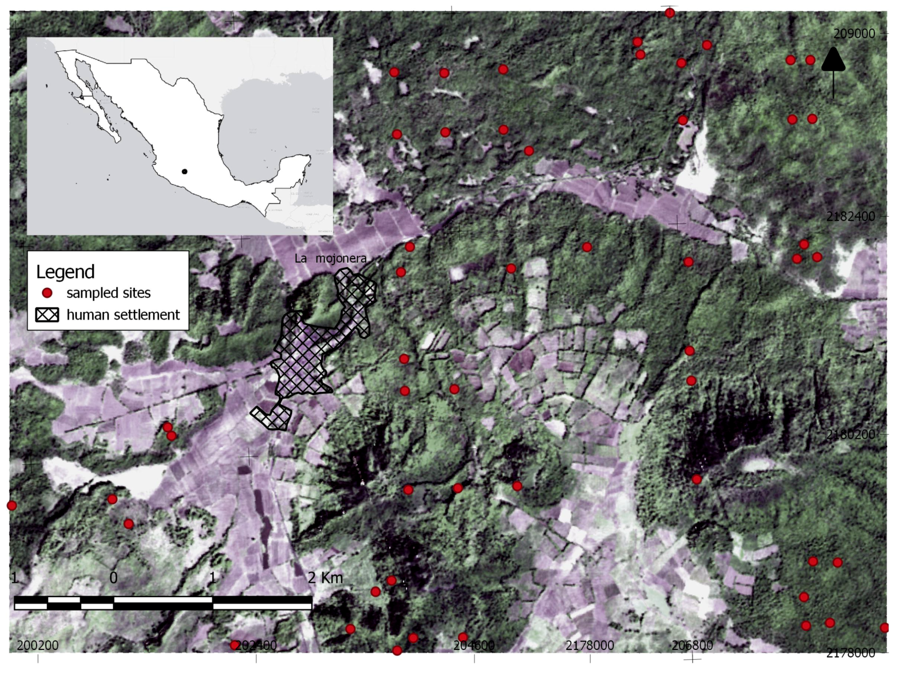
2.1. The Study Area

This study was carried out in an ‘ejido’ of central Mexico (19 44’00” N, 101 52’00” W) with an altitude between 2300 and 3300 m.a.s.l. The study area was mountainous with highly porous volcanic soil. It has a sub-humid temperate climate that rains in summer with a temperature varying between 10 C and 15 C. The average annual precipitation is about 1274 mm that concentrates in the months from June to October. The vegetation is comprised mainly of pine–oak forest that dominates in the Mexican transition zone in the central part of the country that forms part of the study area. The intensive use of wood and a lack of forest management plan in the last three decades have caused the decline of the forest cover in the study area.

2.2. Fieldwork Data

Field data collection was carried out under the scheme of a participatory forest inventory carried out by local inhabitants. In this sense, the dates for the inventory by local inhabitants were determined based on the best time of year to sample the forest. Thus, the dates for the participatory forest inventory were specified in two periods, June 2013 and October 2014. The participatory forest inventory was carried out using a non-aligned systematic sampling design.
Seven structural parameters of the forest were measured in 52 circular plots of 500 m 2 each in a nested type (radius of 12.62 m) with a concentric circle of 100 m 2 (Figure 1). For each plot, trees with diameter of breast height (DBH) >5 cm and the regeneration of trees with 5 m > DBH > 2.5 cm were measured. The AGB obtained from the terrestrial inventory data were used as a dependent variable in the regression analysis. To estimate the AGB with the surveyed data, allometric equations from the literature were used, adapted for the forest genus that characterize the temperate forest in the Mexican Transition zone (Table 1).

2.3. Satellite Images

One scene of the multiespectral SPOT-5 from 9 February 2014 was obtained, with four spectral bands (green: 500–590 nm, red: 610–680 nm, near infrared ( N I R ): 780–890 nm, mid-infrared: 1580–1750 nm) and a spatial resolution of 10 m in the multispectral bands and 2.5 m in the panchromatic band (Figure 2). The scene was orthorectified using control points extracted from the orthophotos with spatial resolution of 2 m and from the digital elevation model with spatial resolution of 15 m. Also, one scene of the RapidEye sensor (orthorectified) from 15 February 2013 was obtained with five spectral bands (blue: 440–510 nm, green: 520–590 nm, red: 630–685 nm, red edge: 690–730 nm, and near infrared ( N I R ): 760–850 nm), and 5 m spatial resolution. Both SPOT-5 and RapidEye images were corrected atmospherically and topographically with the ATCOR3 module which is a radiometric correction method suitable for mountainous areas [48].

2.4. Independent Variables

From each satellite image, the potential variables were obtained to explain the AGB estimated by the field survey data. The spectral values of the five bands of the RapidEye sensor and the four bands of the SPOT-5 image were explored, and the principal components were calculated. Based on the spectral bands, thirteen vegetation indices (Table 2) and four variables of elevation model (altitude, slope, orientation and solar radiance) were generated. For each spectral band, eight indices of GLCM (grey-level co-occurrence matrix) textures, namely mean, variance, correlation, dissimilarity, entropy, second moment, contrast and homogeneity, were calculated using the package ‘glcm’ of the statistical software R [49]. To calculate the texture information, various window sizes were experimented (from 3 × 3 to 15 × 15 pixels) [9]. The optimal window size for the calculation of the texture information was selected based on the correlation with the AGB; for SPOT 5 image, the optimal window size that allowed for the highest correlation coefficient is 7 × 7 and for RapidEye it is 3 × 3. The texture index has been widely cited in the literature for having a strong association with structural forest parameters [50,51,52] and AGB [53]. The computing of these metrics resulted in 55 variables derived from the SPOT-5 image (See Table A1) and 67 from the RapidEye image (See Table A2). In a first step, a correlation analysis was made to these variables and the less significant variables were discarded based on critical correlation values from Pearson and the number of data sampled [54]. In a second step, regression models were generated under the two approaches proposed in this study, Stepwise with AIC and techniques of relative importance, selecting the regression model with the best performing explanatory variables.

2.5. Statistical Methods

2.5.1. Correlation Analysis and Model Assumptions

The Pearson correlation coefficient analysis was carried out to select the variable with the highest coefficient and to discard the presence of multi-collinearity in the group of the textural variables and the vegetation indices. In this way, the variables with the highest coefficient were selected and the total number of variables used in the equation was reduced. Afterwards, the remaining variables proposed initially were included and those related significantly (p-value < 0.05 and < 0.01 ) with the AGB were selected. The statistical test of normality (Shapiro–Wilk) and the homoscedasticity of the residuals models (Breush–Pagan) were applied, and the calculation of the inflation factor of the variance was carried out to detect the possible problems of the multicollinearity between independent variables. In order to eliminate the heteroscedasticity or the lacking of the normality in the residuals, transformation of the dependent variable was carried out. Diagnostic graphics and the distance Cook were carried out to identify the observations with high residual values or possible leverages and a robust regression analysis [68,69].

2.5.2. Variable Selection Methods

The methods of STEPWISE-AIC and RI were applied to select the appropriate explanatory and predictive variables. Both methods were implemented in the statistical software R with the packages ‘stats’ and ‘relaimpo’ [70,71]. The method by steps (STEPWISE) has been widely used for the selection of variables by being easily managed and widely extended to more generalized models (e.g., linear/non-linear models, abnormal data distribution) [31]. On the other hand, the criterion of the Akaike (AIC) provides the model and the maximum likelihood estimation of the parameters and gives the minimum of the A I C [72]. The criterion of the Akaike is defined as Equation (1).
A I C = 2 l n L [ θ ^ ( k ) ] + 2 k ,
where L [ θ ^ ( k ) ] is the likelihood function of the observations, θ ^ ( k ) is the maximum likelihood estimation of the parameter vector θ , k is the number of the adjusted independent parameters within the model, and l n denotes natural logarithm [73]. When comparing various models, the parameters estimated by the maximum likelihood method and the AIC values are calculated and compared in order to find a model with the minimum AIC value. This procedure is called the minimum AIC procedure [74]. Thus, the most reliable model is the less complicated one, or the one with a major information gain. In this case, transformation of the AIC method in the form of STEPWISE was used and the best model with the lowest AIC value was selected in function with the AGB variable for the two types of satellite images.
The relative importance of an explanatory variable in a regression model is defined as the proportional contribution of each predictor for R 2 , considering both direct effect (meaning its correlation with the criterion) and the effect when combined with other variables in the regression equation [32]. In this study, three relative importance matrices were used: the proportional marginal decomposition ( P M V D ), the simple marginal decomposition ( L M G ) and the FIRST metric. P M V D is defined as the weighted average of the contributions of the regressors in the model, in which each order of those receives a weight depending on the data [37,39]. It is defined as Equation (2):
P M V D ( x k ) = 1 ( p ! ) r p e r m u t a t i o n s p ( r ) s e q R 2 x q r .
where p ( r ) is the weight and s e q R 2 is the explained variance of the model added sequentially.
L M G is defined as the average of the contributions of all the orders of the regressors, based on the sum of the squared sequential of the linear model whose size depends on the order of the regressor in the model. A global evaluation is obtained by averaging an overall assessment of all systems of the regressors [35]. This metric is defined as Equation (3):
L M G ( x k ) = 1 ( p ! ) r p e r m u t a t i o n s s e q R 2 x q r .
In this method, the same weight is given to each order of the regressors. This method has been used as hierarchical partition, generalized by Chevan and Sutherland [36]; Walsh and MacNally [75] provided a package in the software R (hier.part) using this approach. In the present study, the similarities of the P M V D and L M G weights were evaluated to select regressors without correlation based on the studies of Gromping [38] and Gromping [39] that demonstrate that the L M G and P M V D weights coincide for the uncorrelated regressors, provided that the coefficients β of the regressors are very similar or have correlations close to 0. Otherwise, the regressors were selected based on the weights of the P M V D and F I R S T metrics.
F I R S T is a simple RI metric that denotes the R 2 that explains the regressor on its own. This metric was equivalent to calculating the square of the regressor correlation with the response variable [38]. If the regressors were correlated, the sum of these individual contributions was higher than the total of the R 2 of the model with all the regressors together. One way to see the relative importance was to compare which regressor alone was able to explain the model, comparing the R 2 of the regression models with a single regressor. In this study, F I R S T was used to evaluate the weight of the regressors for the case in which all regressors are correlated. The regressor with the highest F I R S T weight was selected.
The package ‘relaimpo’, in the software R, uses six metrics (first, last, betasq, pratt, pmvd y lmg) to evaluate the relative importance of the variables in a linear model; of those, this study used first ( F I R S T ), pmvd ( P M V D ) and lmg ( L M G ) metrics.

2.5.3. Validation of the Regression Models

To evaluate the explanatory and predictive performance of the model, a crossed validation approach was applied [76], which was the most practical way to predict and evaluate the error rate in the biomass estimation models [30], and applied when the quantity of the data for training and testing is limited [77,78].
A variation of this approach was the method of triple cross validation (TFOLD), in which the data were divided in three approximately equally sized partitions; each one was used for testing and the rest of the data were used for training. This procedure was repeated three times in a way that in the end all the cases were used only once for the testing. To obtain a reliable performance in the prediction of the regression models, the TFOLD procedure was repeated 10 times, reorganizing and stratifying the data before each round [79].
The validation results were evaluated by the mean absolute percentage error (MAPE), proposed by Sileshi [30] widely used in the prediction and comparison of the ecological and environmental evaluation models. The MAPE is defined by the following Equation (4):
100 n i = 1 n M o M p M o ,
where M o and M p are observed and predicted biomass values, respectively, and n is the number of sampling sites. The explanatory model was selected with the lowest MAPE using all the data sets and in addition cross-validation was applied to evaluate the variables of the learning model [80]. To evaluate the predictive variables, the models were generated with the variable selection methods within the triple crossed validation methods in order to compare the MAPE results between the variable selection methods.

3. Results

3.1. State and Structure of the Forest

A summary of the basic information obtained from the analyses described above is given in Table 3. During the field campaign, eight forest genus with the highest AGB values were sampled. The percentage of each sampled forest genus was Pinus 44%, Quercus 35%, Alnus 15%, Cupressus 3%, Arbutus 2% and the rest of the genus 1%. In total, 79% of the AGB was represented by the first two genus.

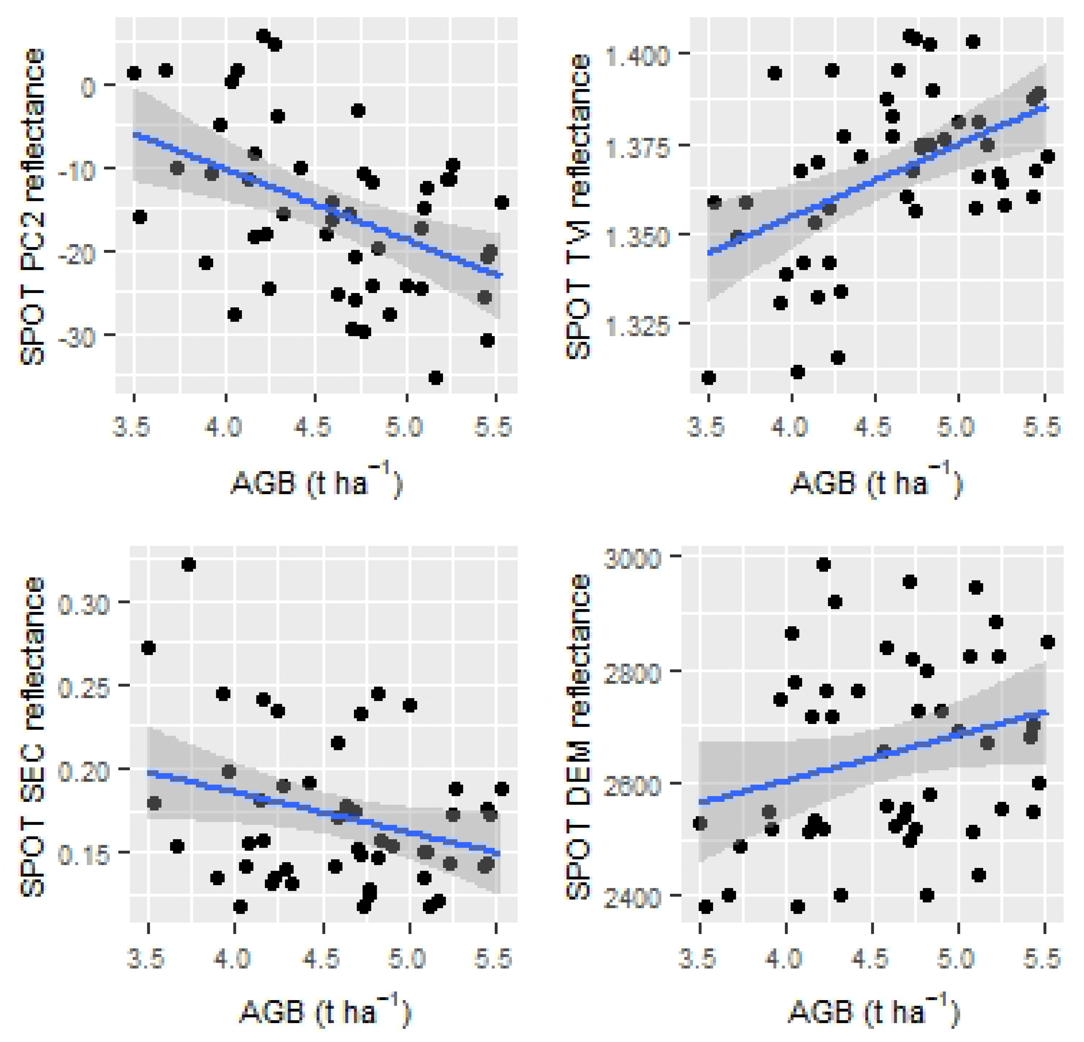
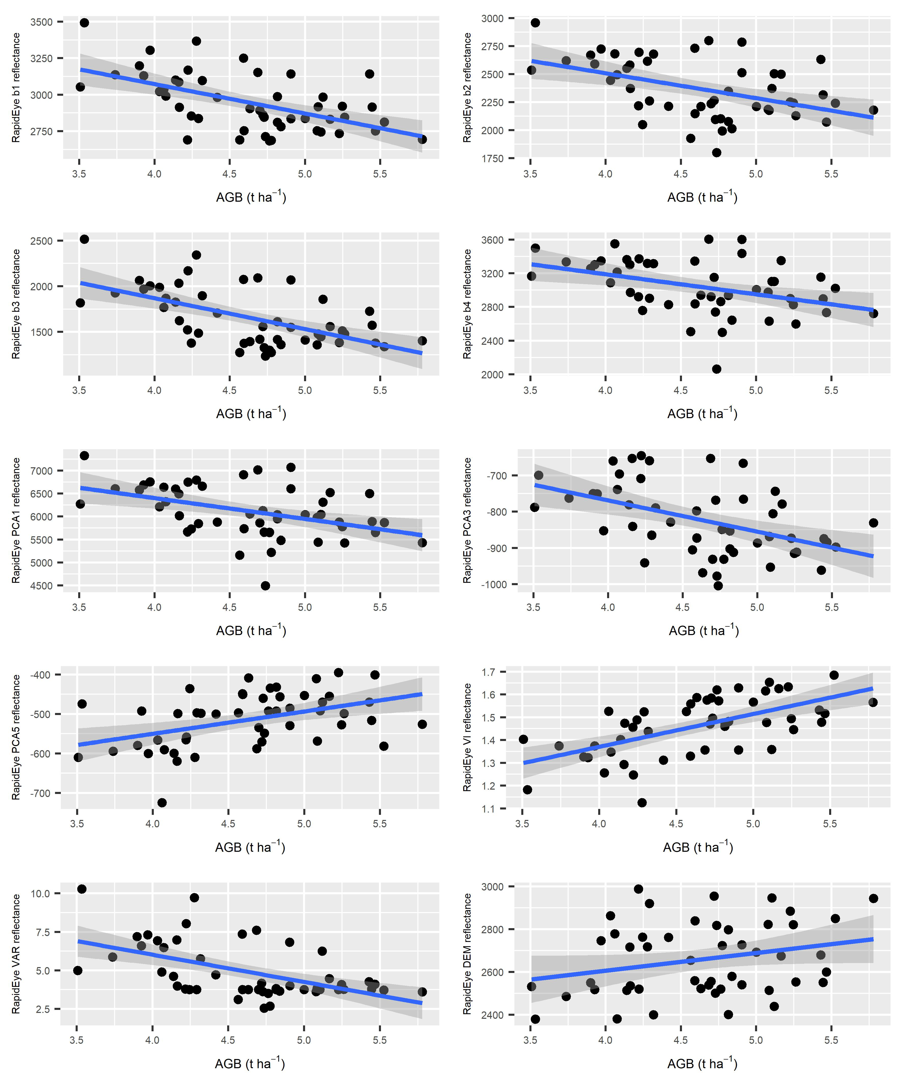
3.2. Correlation Analysis

From the 55 variables (See Table A1) derived from the SPOT-5 images, only four variables were significantly correlated (Table 4) with AGB (AGB-Spot5), based on critical values for Pearson’s Correlation [81] (Figure 3) and 10 variables from the 67 derived (See Table A1) from the RapidEye images (AGB-RapidEye).
For SPOT-5 image, the variable principal component 2 (PC2) shows the highest correlation with the AGB and for the RapidEye image it was the variable green–red vegetation index (VI) (Figure 4). The correlation between AGB and the variables derived from the RapidEye image presented the highest correlation coefficients. The spectral bands of the SPOT-5 images did not have a significant correlation with the AGB while the RapidEye images obtained high and negative coefficients with the first four spectral bands (blue, green, red and red edge). Of the principal components for the RapidEye image, the principal component 5 (PC5) showed the highest coefficient with 0.535, while for the SPOT-5 image, only the principal component 3 (PC3) showed a significant coefficient of −0.320. The transformed vegetation index (TVI) from the SPOT-5 image was significantly correlated with AGB (0.276) and green–red VI from RapidEye image showed a significant coefficient of 0.535 with AGB. The texture indices that had a significant correlation with AGB were the second moment NIR (SEC) from Spot5 and variance red (VAR) from RapidEye. The altitude variable from both images enabled significant results. Satellite Images

3.3. Estimation of the AGB

The initially selected variables through linear regression and the adjustments of the regression models by the variable selection method are shown (Table 5) for each image. All the estimated parameters were significant ( p value < 0.1 , p < 0.05 or p < 0.01 ).
STEPWISE-AIC selected three explanatory variables for the SPOT-5 image and five for the RapidEye image, while RI selected three for the SPOT-5 image and two for the RapidEye image (Table 5). The model that showed the highest determination coefficient R 2 and lowest standard residual errors (SRE) were the models generated from the RapidEye image for both STEPWISE-AIC ( R 2 = 0.437, SRE = 0.431) and RI ( R 2 = 0.420, SRE = 0.423) proposed approaches. The models with the lowest R 2 and highest SRE were for the models generated with variables of the SPOT-5 image for both STEPWISE-AIC ( R 2 = 0.359, SRE = 0.451) and RI ( R 2 = 0.359, SRE = 0.451) proposed approaches. The variables derived from the SPOT-5 image that enabled significant results for both selection methods were TVI, SEC Y DEM, while for the RapidEye image the variables were the red band, red edge, some of the principal components for the estimated model with the STEPWISE-AIC method and the component CP5 and VI with the method RI.
The fitted data of the models are shown in Figure 5. They were identified as lacking normality and homoscedasticity, caused by the symmetry found in the distribution of the samples in all the regression models with the original variables, and they were eliminated by transforming the variables to the format of the natural logarithm. The analysis of the outlier values and the leverage in the observations and the robust regression analysis showed that three observations had a notable effect in the adjustment of the models. Two observations with very low AGB values were found in the areas of the open forest and so the reflectance value does not correspond only to the forest. One observation was represented by a very high AGB value located in a private plot with the trees designated to rubber extraction (trees with more than 100 cm of the DBH and older than 70 years).

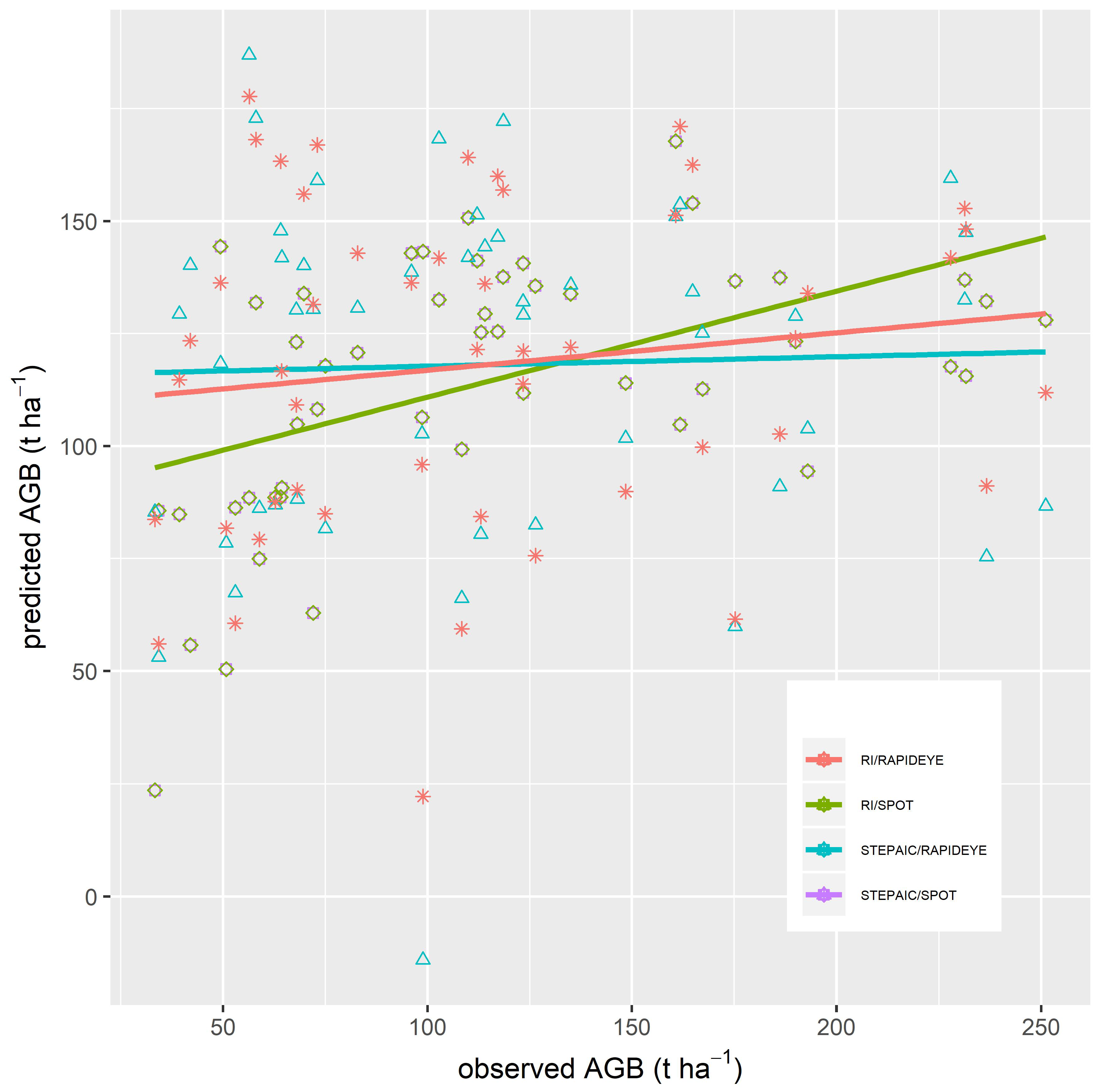
3.4. Validation of the Regression Models

The results of the triple cross validation of the regression models are shown in Table 6. From SPOT-5, the lowest MAPE value was 38.04 in both methods, and the range between MAPE values was 5.17. From RapidEye, the lowest MAPE was 34.47 in the RI method, and the range between MAPE values was 11.71. Comparing the two sensors, RapidEye showed lower MAPE values and a smaller range than SPOT-5. Among the methods used with the RapidEye sensor, the RI method obtained the lowest MAPE values.
The results of the selection of variables and generation of the regression model within the triple cross validation for both images are shown in Table 7 and Table 8. For the SPOT-5 image with the STEPWISE-AIC approach, the minimum MAPE value obtained was 29.44 with three selected variables and the maximum MAPE value obtained was 62.36 with four selected variables and a range between MAPEs of 32.92. for the SPOT-5 image with the RI approach. The minimum MAPE value obtained was 29.44 with three selected variables and the maximum MAPE value obtained was 57.94 with three selected variables and a range between MAPEs of 28.5. For the RapidEye image with the STEPWISE-AIC approach, the lowest MAPE value obtained was 31.86 with five variables selected and the maximum MAPE obtained was 64.54 with seven variables selected. For the RapidEye image with the RI approach, the lowest MAPE value obtained was 30.73 with a variable selected and the maximum MAPE value obtained was 56.63 with two variables selected and a range between MAPEs of 25.9.

4. Discussion

4.1. Correlation Analysis

The correlations between the AGB and four variables for the SPOT-5 images and ten variables for the RapidEye images were significant (p value < 0.1 , p < 0.05 or p < 0.01 ), though not particularly high. The bands of blue, green, red, and red edge of the RapidEye image showed a significant correlation with the AGB, especially the red band that had the highest correlation coefficient (−0.511) compared with the rest of the multispectral bands. It is shown that the visible spectral bands of the RapidEye image and the band of the red edge can be sensitive to the reflectance with the AGB. No studies were found in which the multispectral bands of the RapidEye image were included as predictive variables for biomass estimation, however, studies such as Ojoyi et al. [82] estimated the AGB with a vegetation index that included those bands as predictive variables and Wallner et al. [16] estimated the parameters of the forest structure using the visible spectral bands and the vegetation indices. The 7 × 7 second moment NIR (SEC) variable from SPOT-5 image and the 3 × 3 Variance Red Texture (VAR) variable from RapidEye image showed a significant correlation (Table 4), independently of not being selected in any regression model. This is consistent with Wallner et al. [16] and Castillo-Santiago et al. [9] that texture information is related to AGB when using SPOT-5 images and RapidEye images and can improve results as variables in regression models.
The 3 × 3 variance red texture (VAR) variable from the RapidEye image showed the highest correlation in the correlation analysis. However, it was not selected in the regression models with any approach because there is a strong dependence on VAR with the Red Band and green–red vegetation index (VI); these variables showed a higher correlation coefficient than VAR. It is the opposite case for variables selected from the SPOT-5 image, in which the models selected the variables in the absence of collinearity between independent variables, caused by the reduced set of variables that resulted from the previous correlation analysis. We conclude that texture information can improve AGB estimates in mixed forests based on three considerations: (1) correlation analyses of the variables generated by both SPOT-5 and RapidEye images show texture variables with high correlation coefficients and therefore, potentially suitable variables for a multiple regression model for the estimation of AGB; (2) in both models and in the absence of collinearity, the textural variable second moment NIR (SEC) of the SPOT-5 image was selected, even with a low correlation coefficient, which tells us the importance of this variable together with the other variables in a multiple regression model; otherwise, it would have been discarded; (3) similar studies such as Wallner et al. [16] and Castillo–Santiago et al. [9] indicate the relevance of textural variables in estimates of AGB and structural parameters. The principal components (PCs) showed a high correlation for both images. The sensibility of the reflectance in the PCs for the identification of the variation of both the vegetation and the biomass is demonstrated [83,84]. It is also proved that the PC bands from the high spatial resolution images such as RapidEye can be useful to estimate the AGB. Tian et al. [21] confirmed that PC bands can be used as variables, in combination with other predictive variables, to estimate the AGB. The vegetation indices were significant with AGB (TVI for the SPOT-5 image and VI for the RapidEye image) by being narrowly related with the quantity of the chlorophyll and the vegetation structure, such as the VI calculated by the green and the red bands in which the vegetation reflects and absorbs the electromagnetic radiation by the pigment of the plants and the TVI calculated by the red and NIR bands, in which the reflectance is controlled by the plant structures [85]. In this study, the high values of the two indices—TVI and VI—indicate the increase of the forest density. This finding was supported by the studies of Aguirre–Salado et al. [11], Aguirre–Salado et al. [86], and Muñoz–Ruiz et al. [87], for temperate forest with similar characteristics. This study showed the high sensibility of the vegetation indices generated by the RapidEye image for AGB estimation. As expected, the topography has an effect on the biomass distribution of mixed pine–oak forests, which is confirmed by the models generated by variables from the SPOT-5 image that include DEM as a predictive variable. The results of this study are consistent with those from the studies of Ojoyi et al. [82] and Xie et al. [20].

4.2. Estimation of the AGB

Studies that predict the structural variables of the forest and the AGB generally report the determination coefficient of R 2 and/or the root mean squre error (RMSE) as indicators of the adjustment of the correlation between the variables derived from the satellite images and those measured from the field survey. In this study the results obtained from the regression models for the SPOT-5 and RapidEye images are within or nearest the fit ranges of models in studies estimating AGB and forest structural parameters implemented with different methodologies. Estimates with determination coefficients between 0.45–0.69 in the Tian et al. [21] study using variables derived from the SPOT 5 image and variables derived from other sources, 0.44–0.60 in the Ojoyi et al. [82] study using topo-edaphic variables and vegetation indices derived from the RapidEye image and 0.19–0.63 in the Wallner et al. [16] study using texture variables derived from the RapidEye image. Other studies closely related to the conditions of the study area, for example the Aguirre–Salado et al. [86] study obtained determination coefficients between 0.14–0.76 and the Zhao et al. [27] study obtained values between 0.34–0.53. However, in our study the low results of R 2 values is because of a fewer set of ground plots, with respect to AGB variability, which depend on: (1) the generalization in the age and size of the trees in the allometric equations with which the aerial biomass was estimated and the restriction of the range that includes only a part of the tree [30]; (2) the shadows generated due to the mountainous relief of the region mask trees with wide canopies [88] and the fragmentation of the forest combined with the lack of management in the study area which increases the error and therefore decreases the R 2 ; (3) the date of acquisition of the satellite images were slightly different from the date of the field survey, introducing the seasonal effect. In this study the dates of acquisition of images were in February and the survey was carried out in June and October; (4) the collection of data unstratified in the plots causes biased estimates of standard errors and decreases the total variance explained in the model [17]. However, they could improve by increasing the size of the sample and applying a stratification by forest type [16,17].
The “stepwise” method and the criterion of the Akaike (AIC) have been utilized to select variables in factorial analysis, regression models and time series analysis [20,21,25,89,90]. One of the limitations of applying AIC is that when using small- or medium-sized samples, it tends to select more parameters than are necessary [91]. Also, it assumes independence between variables and, sometimes, it can generate regression models with high R 2 but that explain the variable of interest poorly due to multi-collinearity. This study shows that, for the RapidEye image, the STEPWISE-AIC method selected five parameters, in comparison with the RI method, which selected only two parameters; it has a lower R 2 , but obtained a higher adjusted R and lower Residual Error. In the case of the SPOT-5 image, most of the variables were discarded in the correlation analysis and a reduced set of explanatory variables was used. The metrics in the analysis of relative importance allow the quantification of the contribution of a regressor in a multiple regression model and have been applied by various authors [32,37,40,70,75]; however, in this study, these metrics were used to select the best predictive variables according to the contribution to the regression model, to reduce the number of parameters and also to eliminate the multi-collinearity phenomenon. The combination of the metrics of relative importance used in this study can help to select independent predictive variables that allow regression models with acceptable fitting to be generated.

4.3. Validation of the Regression Models

The predictive capacity of the regression models generated with the proposed approaches was compared based on their MAPE and the evaluation of the spectral response between the SPOT-5 and RapidEye images. For both SPOT-5 and RapidEye images, AGB estimation with the RI approach had a generally lower MAPE and smaller dispersion of error values than the STEPWISE-AIC approach, although relatively large RMSE values are displayed in all iterations (Table 6, Table 7 and Table 8). This is explained by the greater forest fragmentation in the unmanaged la Mojonera forest area, which increases the variance in the spectral response of the variables and thus the error. The lower RMSE and MAPE values are most probably due to the smaller range of reference biomass values and the homogeneity (in terms of the volume of the trees) that remains in some areas of the la Mojonera temperate forest. In addition, we observed similar values in terms of the dispersion MAPE values of both images, which indicates that the difference in spatial resolution between five (RapidEye) and 10 (SPOT-5) meters does not influence the explanatory and predictive capacity of the generated biomass models, under the biophysical and management conditions presented in the study area. The minimum and range values in the triple cross validation of this study show that the IR approach for both images can improve the predictive performance of regression models to estimate forest aboveground biomass. The RI approach showed smaller MAPE in each one of the iterations than the STEPWISE-AIC approach. It also selected regression models with fewer variables and, therefore, parsimonious models, thus guaranteeing the absence of collinearity between variables, unlike the STEPWISE-AIC approach, which selected more variables in all the iterations of the cross-validation for both images. The use of MAPE in this study limited the comparison with other methods of selection of variables used in other studies [30], so it was difficult to define a universal cutoff for what constitutes a large bias (or MAPE), for the selection of the objective model and consistent information, so the lowest MAPE value was chosen as the best model for the estimation of AGB. Regression models are built by randomly selecting a subset of AGB ground plots (calibration set), fitted against satellite derived variables at the same locations so they can be used to produce wall to wall estimates of AGB. The accuracy of regressions models can be tested by comparing regression estimations against the remaining subset of plots (validation set). The form and accuracy of regression models can vary depending on which calibration plots are selected in the first place. The larger the variation, the less reliable are estimations as these will depend to some extent on the selection of calibration plots. By iteratively selecting calibration plots, we built an array of regression models using two methods for variables selections (RI and AIC approaches) and two sensors (RapiEye and Spot-5). However, using the relative importance approach for selecting non-correlated variables resulted in equations with lower errors in average as measured by MAPE.

5. Conclusions

This study compares two methods for selecting independent variables in regression models for estimating aboveground forest biomass in a mixed temperate forest in central Mexico. To our knowledge, the relative importance method is not commonly used for estimating aboveground forest biomass. However, our results suggest that this method could perform better than AIC in situations with few biomass ground plots; something frequent in community managed forests across the global south. Likewise, we consider that both SPOT-5 and RapidEye images can be used to generate predictive variables for the estimation of aboveground forest biomass, under biophysical and management conditions such as those presented in the study area. This study highlights the need to combine field data with remote sensing to obtain cost-effective estimates of aboveground forest biomass. It also highlights the use of appropriate methodologies for the selection of suitable variables to generate accurate predictive models. Since our study shows predictive models for estimating biomass with a reduced set of variables, lower errors and no correlation between predictive variables, it can be concluded that the approach based on relative importance metrics is suitable in estimating aboveground forest biomass. However, the error of the estimates was relatively high, which can be attributed to the mountain relief of the region and the fragmentation of the forest coupled with the lack of management in the study area. It is recommended that stratification by forest type and the generation and insertion of predictor variables from different sensors can considerably improve the results and increase the reliability of the estimates.

Author Contributions

Investigation, R.L.A.-C. and A.G.; methodology, R.L.A.-C. and A.G.; validation, R.L.A.-C. and A.G.; writing—review and editing, Y.G., J.P.-G. and J.-F.M.

Funding

This research has been supported by the project PAPIIT IA101513, UNAM “Análisis geoespacial de la degradación forestal por la extracción de madera para leña y carbón vegetal en el centro de México”, SENER CONACYT 2014 246911 “Clúster de Biocombustibles Sólidos para la Generación Térmica y Eléctrica” and CONACYT Ciencia Básica SEP 285349 “Análisis del patrón de la degradación en selvas y bosques de México con percepción remota en múltiples escalas en el tiempo y espacio”.

Acknowledgments

We acknowledge to the students of the Michoacan Indigenous Intercultural University and inhabitants of the La Mojonera ejido for their collaboration in the field brigades with the collection of valuable information for this work. The first author acknowledges the Consejo Nacional de Ciencia y Tecnología for Grant number 240717.

Conflicts of Interest

The authors declare no conflict of interest.

Appendix A

We analyze the relationship between the dependent variable AGB and the independent variables. Fifty-five potential variables derived from the SPOT-5 image (Table A1) and 67 derived from the RapidEye image (Table A2). The Pearson’s correlation coefficient was calculated for each pair (p-value < 0.05 and < 0.01 ).
Table A1. Independent variables generated from the SPOT-5 image.
Spectral Bands
Green band
Red band
NIR band
SWIR band
Principal Components
Principal component 1 (PC1)
Principal component 2 (PC2)
Principal component 3 (PC3)
Principal component 4 (PC4)
Vegetation indices
Normalized difference vegetation index (NDVI )
NIR/red reflectance ratio index (RATIO)
NIR/green reflectance ratio index (GR)
Green–red reflectance ratio index (VI)
Ratio vegetation index (RVI)
Brightness index (Brightness)
Soil adjusted vegetation index (SAVI)
Transformed vegetation index (TVI)
Corrected transformed vegetation index (CTVI)
Thiam’s transformed vegetation index (TTVI)
Normalized ratio vegetation index (NRVI)
Digital Elevation Model
Altitude
Slope
Orientation
Solar Radiance
7 × 7 GLCM(grey-level co-occurrence matrix) textures per band
Mean (green band, red band, NIR band, and SWIR band)
Variance (VAR) (green band, red band, NIR band, and SWIR band)
Correlation (green band, red band, NIR band, and SWIR band)
Dissimilarity (green band, red band, NIR band, and SWIR band)
Entropy (green band, red band, NIR band, and SWIR band)
Second moment (SEC) (green band, red band, NIR band, and SWIR band)
Contrast (green band, red band, NIR band, and SWIR band)
Homogeneity (green band, red band, NIR band, and SWIR band)
Table A2. Independent variables generated from the RapidEye image.
Spectral Bands
Blue band
Green band
Red band
Red edge band
NIR band
Principal Components
Principal component 1 (PC1)
Principal component 2 (PC2)
Principal component 3 (PC3)
Principal component 4 (PC4)
Principal component 5 (PC5)
Vegetation indices
Normalized difference vegetation index (NDVI)
NIR/red reflectance ratio index (RATIO)
NIR/green reflectance ratio index (GR)
Green–red reflectance ratio index (VI)
Ratio vegetation index (RVI)
Brightness index (Brightness)
Soil adjusted vegetation index (SAVI)
Transformed vegetation index (TVI)
Corrected transformed vegetation index (CTVI)
Thiam’s transformed vegetation index (TTVI)
Normalized ratio vegetation index (NRVI)
Normalized difference red edge (NDRE)
Ratio index (RI)
Digital Elevation Model
Altitude
Slope
Orientation
Solar Radiance
3 × 3 GLCM(grey-level co-occurrence matrix) textures per band
Mean (blue band, green band, red band, NIR band, and red edge band)
Variance (VAR) (blue band, green band, red band, NIR band, and red edge band)
Correlation (blue band, green band, red band, NIR band, and red edge band)
Dissimilarity (blue band, green band, red band, NIR band, and red edge band)
Entropy (blue band, green band, red band, NIR band, and red edge band)
Second moment (SEC) (blue band, green band, red band, NIR band, and red edge band)
Contrast (blue band, green band, red band, NIR band, and red edge band)
Homogeneity (blue band, green band, red band, NIR band, and red edge band)

References

  1. Dixon, R.K.; Brown, S.; Houghton, R.A.R.; Solomon, A.M.; Trexler, M.C.; Wisniewski, J. Carbon pools and flux of global forest ecosystems. Science 1994, 263, 185–190. [Google Scholar] [CrossRef]
  2. Houghton, R.A.; Hall, F.; Goetz, S.J. Importance of biomass in the global carbon cycle. J. Geophys. Res. Biogeosci. 2009, 114, 1–13. [Google Scholar] [CrossRef]
  3. Toan, T.L.; Quegan, S.; Davidson, M. The BIOMASS mission: Mapping global forest biomass to better understand the terrestrial carbon cycle. Remote Sens. Environ. 2011, 115, 2850–2860. [Google Scholar] [CrossRef] [Green Version]
  4. Marta-Pedroso, C.; Laporta, L.; Proença, V.; Azevedo, J.C.; Domingos, T. Changes in the ecosystem services provided by forests and their economic valuation: A review. For. Landsc. Glob. Chang. Chall. Res. Manag. 2014, 3, 107–137. [Google Scholar] [CrossRef]
  5. Timothy, D.; Onisimo, M.; Riyad, I. Quantifying aboveground biomass in African environments: A review of the trade-offs between sensor estimation accuracy and costs. Trop. Ecol. 2016, 57, 393–405. [Google Scholar]
  6. Lu, D.; Chen, Q.; Wang, G.; Liu, L.; Li, G.; Moran, E. A survey of remote sensing-based aboveground biomass estimation methods in forest ecosystems. Int. J. Digit. Earth 2014, 1–43. [Google Scholar] [CrossRef]
  7. Yavasli, D.D. Recent approaches in above ground biomass estimation methods. Aegean Geogr. J. 2013, 21, 39–49. [Google Scholar]
  8. Kayitakire, F.; Hamel, C.; Defourny, P. Retrieving forest structure variables based on image texture analysis and IKONOS-2 imagery. Remote Sens. Environ. 2006, 102, 390–401. [Google Scholar] [CrossRef]
  9. Castillo-Santiago, M.A.; Ricker, M.; de Jong, B.H.J. Estimation of tropical forest structure from SPOT-5 satellite images. Int. J. Remote Sens. 2010, 31, 2767–2782. [Google Scholar] [CrossRef]
  10. Li, W.; Niu, Z.; Liang, X.; Li, Z.; Huang, N.; Gao, S.; Wang, C.; Muhammad, S. Geostatistical modeling using LiDAR-derived prior knowledge with SPOT-6 data to estimate temperate forest canopy cover and above-ground biomass via stratified random sampling. Int. J. Appl. Earth Obs. Geoinf. 2015, 41, 88–98. [Google Scholar] [CrossRef]
  11. Aguirre-Salado, C.A.; Valdez-Lazalde, J.R.; Ángeles-Pérez, G.; de los Santos-Posadas, H.M.; Haapanen, R.; Aguirre-Salado, A.I. Mapeo de carbono arbóreo aéreo en bosques manejados de pino Patula en Hidalgo, México. Agrociencia 2009, 43, 209–220. [Google Scholar]
  12. Du, L.; Zhou, T.; Zou, Z.; Zhao, X.; Huang, K.; Wu, H. Mapping forest biomass using remote sensing and national forest inventory in China. Forests 2014, 5, 1267–1283. [Google Scholar] [CrossRef]
  13. Sousa, A.M.O.; Cristina, A.; Mesquita, P.; Marques, J.R. Biomass estimation with high resolution satellite images: A case study of Quercus rotundifolia. ISPRS J. Photogramm. Remote Sens. 2015, 101, 69–79. [Google Scholar] [CrossRef] [Green Version]
  14. Wani, A.A.; Joshi, P.K.; Singh, O. Estimating biomass and carbon mitigation of temperate coniferous forests using spectral modeling and field inventory data. Ecol. Inform. 2015, 25, 63–70. [Google Scholar] [CrossRef]
  15. Zhu, X.; Liu, D. Improving forest aboveground biomass estimation using seasonal Landsat NDVI time-series. ISPRS J. Photogramm. Remote Sens. 2015, 102, 222–231. [Google Scholar] [CrossRef]
  16. Wallner, A.; Elatawneh, A.; Schneider, T.; Knoke, T. Estimation of forest structural information using RapidEye satellite data. Forestry 2014, 88, 96–107. [Google Scholar] [CrossRef] [Green Version]
  17. Latifi, H.; Fassnacht, F.E.; Hartig, F.; Berger, C.; Hernández, J.; Corvalán, P.; Koch, B. Stratified aboveground forest biomass estimation by remote sensing data. Int. J. Appl. Earth Obs. Geoinf. 2015, 38, 229–241. [Google Scholar] [CrossRef]
  18. Muukkonen, P.; Heiskanen, J. Estimating biomass for boreal forests using ASTER satellite data combined with standwise forest inventory data. Remote Sens. Environ. 2005, 99, 434–447. [Google Scholar] [CrossRef]
  19. Wulder, M.A.; White, J.C.; Fournier, R.A.; Luther, J.E.; Magnussen, S. Spatially Explicit Large Area Biomass Estimation: Three Approaches Using Forest Inventory and Remotely Sensed Imagery in a GIS. Sensors 2008, 8, 529–560. [Google Scholar] [CrossRef] [Green Version]
  20. Xie, Y.; Sha, Z.; Yu, M.; Bai, Y.; Zhang, L. A comparison of two models with Landsat data for estimating above ground grassland biomass in Inner Mongolia, China. Ecol. Model. 2009, 220, 1810–1818. [Google Scholar] [CrossRef]
  21. Tian, X.; Su, Z.; Chen, E.; Li, Z.; van der Tol, C.; Guo, J.; He, Q. Estimation of forest above-ground biomass using multi-parameter remote sensing data over a cold and arid area. Int. J. Appl. Earth Obs. Geoinf. 2012, 14, 160–168. [Google Scholar] [CrossRef]
  22. Lu, D. The potential and challenge of remote sensing-based biomass estimation. Int. J. Remote Sens. 2006, 27, 1297–1328. [Google Scholar] [CrossRef]
  23. Whittingham, M.J.; Stephens, P.A.; Bradbury, R.B.; Freckleton, R.P. Why do we still use stepwise modelling in ecology and behaviour? J. Anim. Ecol. 2006, 75, 1182–1189. [Google Scholar] [CrossRef] [PubMed]
  24. Kronseder, K.; Ballhorn, U.; Böhmc, V.; Siegert, F. Above ground biomass estimation across forest types at different degradation levels in central kalimantan using lidar data. Int. J. Appl. Earth Obs. Geoinf. 2012, 18, 37–48. [Google Scholar] [CrossRef]
  25. Vaglio Laurin, G.; Chen, Q.; Lindsell, J.A.; Coomes, D.A.; Frate, F.D.; Guerriero, L.; Pirotti, F.; Valentini, R. Above ground biomass estimation in an African tropical forest with lidar and hyperspectral data. ISPRS J. Photogramm. Remote Sens. 2014, 89, 49–58. [Google Scholar] [CrossRef]
  26. Duan, Z.G.; Zhao, D.; Zeng, Y.; Zhao, Y.J.; Wu, B.F.; Zhu, J.J. Estimation of the forest aboveground biomass at regional scale based on remote sensing. Geomat. Inf. Sci. Wuhan Univ. 2015, 40, 1400–1407. [Google Scholar]
  27. Zhao, P.; Lu, D.; Wang, G.; Wu, C.; Huang, Y.; Yu, S. Examining spectral reflectance saturation in landsat imagery and corresponding solutions to improve forest aboveground biomass estimation. Remote Sens. 2016, 8, 469. [Google Scholar] [CrossRef]
  28. Lukacs, P.M.; Burnham, K.P.; Anderson, D.R. Model selection bias and Freedman’s paradox. Ann. Inst. Stat. Math. 2010, 62, 117–125. [Google Scholar] [CrossRef]
  29. Ratner, B. Variable selection methods in regression: Ignorable problem, outing notable solution. J. Target. Meas. Anal. Mark. 2010, 18, 65–75. [Google Scholar] [CrossRef]
  30. Sileshi, G.W. A critical review of forest biomass estimation models, common mistakes and corrective measures. For. Ecol. Manag. 2014, 329, 237–254. [Google Scholar] [CrossRef]
  31. Yamashita, T.; Yamashita, K.; Kamimura, R. A Stepwise AIC Method for Variable Selection in Linear Regression. Commun. Stat. Theory Methods 2007, 36, 2395–2403. [Google Scholar] [CrossRef]
  32. Johnson, J.W.; LeBreton, J.M. History and use of relative importance indices in organizational research. Organ. Res. Methods 2004, 7, 238–257. [Google Scholar] [CrossRef]
  33. Johnson, J.W. A Heuristic Method for Estimating the Relative Weight of Predictor Variables in Multiple Regression. Multivar. Behav. Res. 2000, 35, 1–19. [Google Scholar] [CrossRef]
  34. Budescu, D.V. Dominance analysis: A new approach to the problem of relative importance of predictors in multiple regression. Psychol. Bull. 1993, 114, 542–551. [Google Scholar] [CrossRef]
  35. Lindeman, R.H.; Merenda, P.F.; Gold, R.Z. Introduction to Bivariate and Multivariate Analysis; Scott, Foresman: Glenview, IL, USA, 1980; Volume 4. [Google Scholar]
  36. Chevan, A.; Sutherland, M. Hierarchical Partitioning. Am. Stat. 1991, 45, 90–96. [Google Scholar] [CrossRef]
  37. Feldman, B. Relative Importance and Value. SSRN 2005. [Google Scholar] [CrossRef]
  38. Grömping, U. Relative importance for linear regression in R: The package relaimpo. J. Stat. Softw. 2006, 17, 139–147. [Google Scholar] [CrossRef]
  39. Grömping, U. Estimators of Relative Importance in Linear Regression Based on Variance Decomposition. Am. Stat. 2007, 61, 139–147. [Google Scholar] [CrossRef]
  40. Lipovetsky, S.; Conklin, W.M. Predictor relative importance and matching regression parameters. J. Appl. Stat. 2015, 42, 1017–1031. [Google Scholar] [CrossRef]
  41. Chi, H.; Sun, G.; Huang, J.; Guo, Z.; Ni, W.; Fu, A. National Forest Aboveground Biomass Mapping from ICESat/GLAS Data and MODIS Imagery in China. Remote Sens. 2015, 7, 5534–5564. [Google Scholar] [CrossRef] [Green Version]
  42. Lu, D.; Chen, Q.; Wang, G.; Moran, E.; Batistella, M.; Zhang, M.; Vaglio Laurin, G.; Saah, D. Aboveground Forest Biomass Estimation with Landsat and LiDAR Data and Uncertainty Analysis of the Estimates. Int. J. For. Res. 2012, 2012, 1–16. [Google Scholar] [CrossRef]
  43. Foody, G.M. Remote sensing of tropical forest environments: Towards the monitoring of environmental resources for sustainable development. Int. J. Remote Sens. 2003, 24, 4035–4046. [Google Scholar] [CrossRef]
  44. Návar, J. Allometric equations for tree species and carbon stocks for forests of northwestern Mexico. For. Ecol. Manag. 2009, 257, 427–434. [Google Scholar] [CrossRef]
  45. Aguilar, R.; Ghilardi, A.; Vega, E.; Skutsch, M.; Oyama, K. Sprouting productivity and allometric relationships of two oak species managed for traditional charcoal making in central Mexico. Biomass Bioenergy 2012, 36, 192–207. [Google Scholar] [CrossRef]
  46. Acosta, M.; Carrillo, F.; Gómez, R.G. Biomass and Carbon Assessment in Two Tree Species in a Cloudy Forest. Revista Mexicana de Ciencias Agrícolas 2011, 2, 529–543. [Google Scholar]
  47. Norberto Vigil, N. Estimación De Biomasa Y Contenido De Carbono en Cupressus Lindleyi Klotzsch Ex Endl. en El Campo Forestal Experimental “Las Cruces”. Ph.D. Thesis, Universidad Autónoma Chapingo, Texcoco, Mexico, 2010. [Google Scholar]
  48. Neubert, M.; Meinel, G. Atmospheric and Terrain Correction of IKONOS Imagery Using ATCOR3. In Proceedings of the ISPRS Hannover Workshop 2005: High-Resolution Earth Imaging for Geospatial Information, Hannover, Germany, 17–20 May 2005; Volume 3. [Google Scholar]
  49. Zvoleff, A. Calculate Textures from Grey-Level Co-Occurrence Matrices (GLCMs) in R. 2015. Available online: https://rdrr.io/cran/glcm/ (accessed on 20 May 2019).
  50. Lu, D.; Batistella, M. Exploring TM image texture and its relationships with biomass estimation in Rondônia, Brazilian Amazon. Acta Amaz. 2005, 35, 249–257. [Google Scholar] [CrossRef]
  51. Ozdemir, I.; Karnieli, A. Predicting forest structural parameters using the image texture derived from worldview-2 multispectral imagery in a dryland forest, Israel. Int. J. Appl. Earth Obs. Geoinf. 2011, 13, 701–710. [Google Scholar] [CrossRef]
  52. Acevedo, J.A.; Londoño, R.A.; Hernandez, G. Análisis de textura en imágenes de satélite en el ámbito de la biodiversidad y la estructura en un bosque de los Andes Colombianos. Revista Gestión y Ambiente 2008, 11, 137–146. [Google Scholar]
  53. Eckert, S. Improved forest biomass and carbon estimations using texture measures from worldView-2 satellite data. Remote Sens. 2012, 4, 810–829. [Google Scholar] [CrossRef]
  54. Ramsey, P.H. Critical Values for Spearman’s Rank Order Correlation. J. Educ. Stat. 2008, 14, 245–253. [Google Scholar] [CrossRef]
  55. Rouse, J.W. Monitoring the Vernal Advancement and Retrogradation (Green Wave Effect) of Natural Vegetation; NASA: Washington, DC, USA, 1973.
  56. Schneider, T.; Tian, J.; Elatawneh, A.; Rappl, A.; Reinartz, P. Tracing Structural Changes of a Complex Forest by a multiple systems approach. In Proceedings of the 1st European Association of Remote Sensing Laboratories Workshop on Temporal Analysis of Satellite Images, Mykonos, Greece, 23–25 May 2012; pp. 159–165. [Google Scholar]
  57. Jordan, C.F. Derivation of Leaf-Area Index from Quality of Light on the Forest Floor. Ecol. Soc. Am. 1969, 50, 663–666. [Google Scholar] [CrossRef]
  58. Lyon, J.G.; Yuan, D.; Lunetta, R.S.; Elvidge, C.D. A Change Detection Experiment Using Vegetation Indices. Photogramm. Eng. Remote Sens. 1998, 64, 143–150. [Google Scholar]
  59. Kanemasu, E.T. Seasonal Canopy Reflectance Patterns of Wheat, Sorghum, and Soybean. Remote Sens. Environ. 1974, 1974. 3, 43–47. [Google Scholar] [CrossRef]
  60. Definiens. Developer XD 2.0.4. Reference Book; Definiens AG: Munchen, Germany, 2012. [Google Scholar]
  61. Barnes, E.M.; Clarke, T.R.; Richards, S.E.; Colaizzi, P.D.; Haberland, J.; Kostrzewski, M.; Waller, P.; Choi, C.; Riley, E.; Thompson, T.; et al. Coincident detection of crop water stress, nitrogen status and canopy density using ground based multispectral data. In Proceedings of the Fifth International Conference on Precision Agriculture, Bloomington, IN, USA, 16–19 July 2000; pp. 16–19. [Google Scholar]
  62. Huete, A.R. A soil-adjusted vegetation index (SAVI). Remote Sens. Environ. 1988, 25, 295–309. [Google Scholar] [CrossRef]
  63. Deering, D.W.; Rouse, J.W.; Haas, R.H.; Schell, J.A. Measuring forage production of grazing units from landsat MSS data. In Proceedings of the 10th International Symposium of Remote Sensing of Environment, Ann Arbor, MI, USA, 6–10 October 1975; pp. 1169–1178. [Google Scholar]
  64. Perry, C.R.; Lautenschlager, L.F. Funcional Equivalence of Spectral Vegetation Indices. Remote Sens. Environ. 1984, 14, 169–182. [Google Scholar] [CrossRef]
  65. Thiam, A.K.; Khoudiedji, A. Geographic Information Systems and Remote Sensing Methods for Assessing and Monitoring Land Degradation in the Sahel Region: The Case of Southern Mauritania; Clark University: Worcester, MA, USA, 1998; 490p, ISBN 9780591716474. [Google Scholar]
  66. Richardson, A.J.; Wiegand, C.L. Distinguishing vegetation from soil background information. Photogrammetric Engineering and Remote Sensing. Photogramm. Eng. Remote Sens. 1977, 43, 1541–1552. [Google Scholar]
  67. Baret, F.; Guyot, G. Potentials and limits of vegetation indices for LAI and APAR assessment. Remote Sens. Environ. 1991, 35, 161–173. [Google Scholar] [CrossRef]
  68. Li, G. Robust regression. In Exploring Data Tables, Trends, and Shapes; Wiley: New York, NY, USA, 1985. [Google Scholar]
  69. Rousseeuw, P.J.; Leroy, A.M. Robust Regression and Outlier Detection; John Wiley & Sons: Hoboken, NJ, USA, 2005; Volume 589. [Google Scholar]
  70. Grömping, U. Relative Importance of Regressors in Linear Models. Package ‘Relaimpo’. Version 2.2. 2013. Available online: https://www.scribd.com/document/321113503/2013-Package-relaimpo-pdf (accessed on 20 May 2019).
  71. R Core Team. R: A Language and Environment for Statistical Computing; The R Project for Statistical Computing; R Core Team: Vienna, Austria, 2015. [Google Scholar]
  72. Akaike, H. A new look at the statistical model identification. IEEE Trans. Autom. Control 1974, 19, 716–723. [Google Scholar] [CrossRef]
  73. Caballero, F.F. Información en Análisis Factorial. Aspectos Teóricos y Computacionales. Ph.D. Thesis, University of Granada, Granada, Spain, 2011. [Google Scholar]
  74. Bozdogan, H. Model selection and Akaike’s Information Criterion (AIC): The general theory and its analytical extensions. Psychometrika 1987, 52, 345–370. [Google Scholar] [CrossRef]
  75. Walsh, C.; Nally, R.M. Hierarchical Partitioning;R Project For Statistical Computing. 2003. Available online: https://cran.r-project.org/web/packages/hier.part/hier.part.pdf (accessed on 1 February 2019).
  76. James, G.; Witten, D.; Hastie, T.; Tibshirani, R. An Introduction to Statistical Learning; Springer: New York, NY, USA, 2000; Volume 7, p. 618. [Google Scholar]
  77. Witten, I.; Frank, E.; Hall, M.; Pal, C. Data Mining: Practical machine learning tools and techniques; Morgan Kaufmann: Burlington, MA, USA, 2016. [Google Scholar]
  78. Kizha, A.R.; Han, H.S. Predicting aboveground biomass in second growth coast redwood: Comparing localized with generic allometric models. Forests 2016, 7, 96. [Google Scholar] [CrossRef]
  79. Refaeilzadeh, P.; Tang, L.; Liu, H.; Ross, K.A. Cross-Validation. Encycl. Database Syst. 2009, 532–538. [Google Scholar] [CrossRef]
  80. Yao, X.; Wang, S.; Liu, M.; Fu, B.; Lü, Y.; Sun, F. Comparison of Four Spatial Interpolation Methods for Estimating Soil Moisture in a Complex Terrain Catchment. PLoS ONE 2013, 8, e54660. [Google Scholar] [CrossRef] [PubMed]
  81. Statistics Solutions. Table of Critical Values: Pearson Correlation. 2018. Available online: https://www.statisticssolutions.com/table-of-critical-values-pearson-correlation/ (accessed on 1 February 2019).
  82. Ojoyi, M.; Mutanga, O.; Odindi, J.; Abdel-Rahman, E.M. Application of topo-edaphic factors and remotely sensed vegetation indices to enhance biomass estimation in a heterogeneous landscape in the Eastern Arc Mountains of Tanzania. Geocarto Int. 2015, 1–21. [Google Scholar] [CrossRef]
  83. Sheen, S.W. A Principal Component Analysis of Vegetation Characteristics in North America A Principal Component Analysis of Vegetation Characteristics in North America. North 2004, 17, 173–182. [Google Scholar]
  84. Estornell, J.; Martí-Gavilá, J.M.; Sebastiá, M.T.; Mengual, J. Principal component analysis applied to remote sensing. Model. Sci. Educ. Learn. 2013, 6, 83–89. [Google Scholar] [CrossRef] [Green Version]
  85. Campbell, J.B. Introduction to Remote Sensing; Guilford Press: New York, NY, USA, 2002. [Google Scholar]
  86. Aguirre-Salado, C.A.; Treviño-Garza, E.J.; Aguirre-Calderón, O.A.; Jiménez-Pérez, J.; González-Tagle, M.A.; Valdez-Lazalde, J.R.; Miranda-Aragón, L.; Aguirre-Salado, A.I. Construction of aboveground biomass models with remote sensing technology in the intertropical zone in Mexico. J. Geogr. Sci. 2012, 22, 669–680. [Google Scholar] [CrossRef]
  87. Munoz-Ruiz, M.A.; Valdez-Lazalde, J.R.; de los Santos-Posadas, H.M.; Angeles-Perez, G.; Monterroso-Rivas, A.I. Inventory and Mapping of Temperate Forest in Hidalgo, Mexico through Spot and Field Data. Agrociencia 2014, 48, 847–862. [Google Scholar]
  88. Asner, G.P.; Warner, A.S. Canopy shadow in IKONOS satellite observations of tropical forests and savannas. Remote Sens. Environ. 2003, 87, 521–533. [Google Scholar] [CrossRef]
  89. Hero, J.M.; Castley, J.G.; Butler, S.A.; Lollback, G.W. Biomass estimation within an Australian eucalypt forest: Meso-scale spatial arrangement and the influence of sampling intensity. For. Ecol. Manag. 2013, 310, 547–554. [Google Scholar] [CrossRef]
  90. Ene, L.T.; Næsset, E.; Gobakken, T.; Gregoire, T.G.; Ståhl, G.; Nelson, R. Assessing the accuracy of regional LiDAR-based biomass estimation using a simulation approach. Remote Sens. Environ. 2012, 123, 579–592. [Google Scholar] [CrossRef]
  91. Peña, D. Análisis de datos multivariantes; McGraw-Hill España: Madrid, Spain, 2002; p. 515. [Google Scholar]
Figure 1. The location of the study area and the sampling sites.
Ijgi 08 00245 g001
Figure 2. (a) SPOT-5 image with 10 m spatial resolution. (b) RapidEye image with 5 m spatial resolution.
Ijgi 08 00245 g002
Figure 3. Correlations between variables derived from SPOT-5 image and the AGB from the field sample.
Ijgi 08 00245 g003
Figure 4. Correlations between variables derived from a RapidEye image and the AGB from the field samples.
Ijgi 08 00245 g004
Figure 5. The observed AGB against the predicted AGB, determined by variable selection approaches and two satellite images.
Ijgi 08 00245 g005
Table 1. The applied allometric equations for the calculation of the aboveground biomass (AGB).
Common NameGenusAllometric EquationDBH Range (cm) R 2
PinePinusY = 0.1229DBH 2.3964 5.7–57.40.91 [44]
OakQuercusY = 0.0890DBH 2.5226 7.6–62.50.95 [44]
Oak with sproutsQuercusY = 0.0342DBH 2.759 3.8–26.60.94 [45]
TepamoAlnusY = 0.1649DBH 2.2755 10.0–40.00.97 [46]
CedarCupressusY = 0.5266DBH 1.7712 5.0–500.93 [47]
Madroño and other genusArbutusY = 0.0890DBH 2.5226 7.6–62.50.94 [44]
DBH = diameter of breast height.
Table 2. Applied vegetation indices in this study.
Normalized difference vegetation (NDVI) N I R r e d N I R + r e d [55]
Ratio index (RI) g r e e n r e d e d g e r e d [56]
NIR/red reflectance ratio index (RATIO) N I R r e d [57]
NIR/green reflectance ratio index (GR) N I R g r e e n [58]
green–red reflectance ratio index (VI) g r e e n r e d [59]
Brightness b l u e + g r e e n + r e d + r e d e d g e + N I R 5 [60]
Normalized difference red edge (NDRE) N I R r e d e d g e N I R + r e d e d g e [61]
Soil adjusted vegetation index (SAVI) N I R r e d N I R + r e d ( 1 + L ) [62]
Transformed vegetation index (TVI) N I R r e d N I R + r e d + 0.5 [63]
Corrected transformed vegetation index (CTVI) N D V I + 0 . 5 N D V I + 0 . 5 ( N D V I + 0 . 5 ) [64]
Thiam’s transformed vegetation index (TTVI) ( N D V I + 0 . 5 ) [65]
Ratio vegetation index (RVI) r e d N I R [66]
Normalized ratio vegetation index (NRVI) R V I 1 R V I + 1 [67]
Table 3. Descriptive statistics of the variables sampled in the field (n = 52).
ParametersAverageStandard DeviationStandard Error (RMS)MinMax
AGB (ton ha−1 )11666924323
basal area ( m2 ha−1 )1991442
tree height (m)1560432
diameter of breast height (DBH) (cm)22711148
woodland density (trees ha−1)700433571001940
stumps density (stumps ha−1 )163134170480
regeneration height (cm)30202070
Table 4. Correlation coefficients for the linear regression of the AGB comparing with the variables (spectral reflectance, textures, vegetation index, and topographics) derived from SPOT5 and RapidEye images.
VariablesSPOT-5RapidEye
Blue band −0.489 **
Green band −0.393 **
Red band −0.511 **
Red edge −0.323 *
Principal component 1 (PC1) −0.354 **
Principal component 2 (PC2)−0.320 *
Principal component 3 (PC3) −0.423 **
Principal component 5 (PC5) 0.423 **
Green–red vegetation index (VI) 0.535 **
Transformed vegetation index (TVI)0.276 *
3 × 3 variance red texture (VAR) −0.486 **
7 × 7 second moment NIR (SEC)−0.247 *
Altitude (DEM)0.275 *0.275 *
* p-value < 0 . 05 , ** p-value < 0 . 01 .
Table 5. Variables selected from both SPOT-5 and RapidEye images by STEPWISE-Akaike information criterion (AIC) and relative importance (RI) approaches for AGB regression models.
VariablesSPOT-5 ImageRapidEye Image
STEPWISE-AICRISTEPWISE-AICRI
Red band 0.005 (0.003)
Red edge 0.012 * (0.006)
PC1 -0.008 * (0.004)
PC3 -0.008 * (0.004)
PC5 0.011 ** (0.005)0.002 (0.001)
TVI11.032 *** (2.768)11.032 *** (2.768)
VI 2.195 *** (0.523)
SEC−3.075 ** (1.484)−3.075 ** (1.484)
DEM0.001 * (0.0004)0.001 * (0.0004)
Constant−11.966 ***−11.966 ***7.645 ***2.365 **
Observations49494949
R 2 0.3590.3590.4370.420
Adjusted R 2 0.3170.3170.3170.394
Standard residual error (SRE)0.451 (df = 45)0.451 (df = 45)0.431 (df = 43)0.423 (df = 46)
F statistics8.414 *** (df = 3; 45)8.414 *** (df = 3; 45)6.668 (df = 5; 43)16.632 *** (df = 2; 46)
STEPWISE-AIC: the stepwise method based on AIC approach. RI: the relative importance approach.
Table 6. Root mean square error (RMSE) and mean absolute percentage error (MAPE) of the triple crossed validation from the regression models by replica for images of RapidEye and SPOT-5.
RapidEye Image
IterationSTEPWISE-AICRI
RMSEMAPERMSEMAPE
155.7740.9755.6038.08
258.8944.6158.3940.56
368.5344.2561.7841.61
457.7539.1158.7439.54
557.8941.9356.9638.19
664.2146.1853.4134.47
754.3939.3357.4939.65
856.2138.1853.7335.77
954.9238.1853.5035.59
1055.3739.6954.0638.71
SPOT-5 image
IterationSTEPWISE-AICRI
RMSEMAPERMSEMAPE
155.7939.5155.7939.51
256.4640.2456.4640.24
361.2043.2161.2043.21
459.4041.7759.4041.77
558.2540.8958.2540.89
656.8538.3856.8538.38
755.6638.0455.6638.04
859.1539.8159.1539.81
956.0739.1756.0739.17
1057.6740.1257.6740.12
STEPWISE-AIC: the stepwise method based on the AIC approach. RI: the relative importance approach.
Table 7. Regression models generated with STEPWISE-AIC and RI in the triple cross validation and corresponding MAPE for the SPOT-5 image.
IterationSTEPWISE-AICMAPEIterationRIMAPE
Fold 1
1AGB ∼ PC250.591AGB ∼ PC2 + DEM44.32
2AGB ∼ TVI + DEM30.362AGB ∼ TVI + DEM30.36
3AGB ∼ TVI + SEC + DEM53.843AGB ∼ TVI + SEC + DEM53.84
4AGB ∼ PC2 + SEC + DEM45.124AGB ∼ PC2 + SEC + DEM45.12
5AGB ∼ TVI + DEM38.655AGB ∼ TVI + SEC + DEM32.6
6AGB ∼ TVI + SEC45.486AGB ∼ TVI + SEC45.48
7AGB ∼ TVI + DEM52.627AGB ∼ TVI + SEC + DEM45.61
8AGB ∼ PC246.668AGB ∼ PC2 + SEC41.87
9AGB ∼ TVI + DEM45.289AGB ∼ TVI + DEM45.28
10AGB ∼ PC2 + DEM37.9710AGB ∼ PC2 + SEC + DEM36.36
Fold 2
1AGB ∼ TVI + SEC43.791AGB ∼ TVI + SEC43.79
2AGB ∼ TVI + SEC + DEM29.442AGB ∼ TVI + SEC + DEM29.44
3AGB ∼ PC2 + DEM55.613AGB ∼ PC2 + SEC+ DEM54.56
4AGB ∼ TVI + DEM52.794AGB ∼ TVI + SEC + DEM49.52
5AGB ∼ TVI + SEC + DEM54.425AGB ∼ TVI + SEC + DEM54.42
AGB ∼ PC2 + DEM35.436AGB ∼ PC2 + DEM35.43
7AGB ∼ PC2 + SEC + DEM43.037AGB ∼ PC2 + SEC + DEM43.03
8AGB ∼ PC2 + TVI + SEC + DEM53.518AGB ∼ PC2 + SEC + DEM54.27
9AGB ∼ PC2 + SEC + DEM47.579AGB ∼ PC2 + SEC + DEM47.57
10AGB ∼ PC2 + SEC + DEM48.3410AGB ∼ PC2 + SEC +DEM48.34
Fold 3
1AGB ∼ TVI + SEC + DEM42.541AGB ∼ PC2 + SEC + DEM41.17
2AGB ∼ PC2 + TVI + SEC + DEM62.362AGB ∼ PC2 + SEC + DEM57.94
3AGB ∼ TVI + SEC31.943AGB ∼ TVI + SEC31.94
4AGB ∼ PC2 + SEC40.864AGB ∼ PC2 + SEC40.86
5AGB ∼ PC2 + DEM43.335AGB ∼ PC2 + SEC + DEM41.59
6AGB ∼ TVI + SEC + DEM49.656AGB ∼ TVI + SEC + DEM49.65
7AGB ∼ TVI + SEC + DEM38.847AGB ∼ TVI + SEC + DEM38.84
8AGB ∼ TVI + DEM31.338AGB ∼ TVI + DEM31.33
9AGB ∼ TVI + SEC49.829AGB ∼ TVI + SEC49.82
10AGB ∼ TVI + SEC + DEM51.4710AGB ∼ TVI + SEC + DEM51.47
STEPWISE-AIC = The stepwise method based on AIC approach; RI = The relative importance approach; AGB: aboveground biomass; PC2: principal component 2; DEM: altitude; TVI: transformed vegetation index; SEC: 7 × 7 second moment NIR.
Table 8. Regression models generated with STEPWISE-AIC and RI in the triple cross validation and corresponding MAPE for the RapidEye image.
IterationSTEPWISE-AICMAPEIterationRIMAPE
Fold 1
1AGB ∼ b3 + b4 + PC1 + PC3 + PC5 + VAR + DEM62.041AGB ∼ VI + b3 + PC1 + PC552.93
2AGB ∼ b4 + PC1 + PC539.142AGB ∼ b4 + PC3 + PC539.14
3AGB ∼ b3 + b4 + PC1 + PC3 + PC5 + VI + VAR59.463AGB ∼ b3 + PC556.63
4AGB ∼ b3 + b4 + PC1 + PC3 + PC5 + VAR + DEM38.124AGB ∼ VI + b4 + VAR + DEM32.07
5AGB ∼ b4 + PC1 + PC3 + PC538.615AGB ∼ VI + b442.35
6AGB ∼ b3 + PC1 + PC5 + VI55.966AGB ∼ VI41.97
7AGB ∼ b3 + b4 + PC1 + PC3 + PC534.267AGB ∼ VI + PC539.65
8AGB ∼ b3 + b4 + PC1 + PC3 + PC539.438AGB ∼ VI + b3 + PC1 + PC544.03
9AGB ∼ b4 + PC1 + PC3 + PC545.239AGB ∼ VI + PC544.38
10AGB ∼ b4 + PC1 + PC3 + PC5 + VAR42.4510AGB ∼ VI33.47
Fold 2
1AGB ∼ b4 + PC1 + PC544.431AGB ∼ b3 + PC543.52
2AGB ∼ b3 + b4 + PC1 + PC3 + PC559.522AGB ∼ VI48.01
3AGB ∼ b3 + b4 + VI35.473AGB ∼ VI + DEM30.14
4AGB ∼ b3 + b4 + PC1 + PC3 + PC5 + VI51.704AGB ∼ VI + PC1 + PC555.98
5AGB ∼ b3 + b4 + PC1 + PC3 + PC5 + VI54.645AGB ∼ b3 + b4 + PC1 + PC3 + PC5 + VI54.64
6AGB ∼ b3 + b4 + PC1 + PC3 + PC5 + DEM40.266AGB ∼ VI + PC5 + DEM34.56
7AGB ∼ b3 + b4 + PC1 + PC3 + PC5 + VAR + DEM39.287AGB ∼ VI + PC5 + DEM33.49
8AGB ∼ b3 + b4 + PC1 + PC3 + PC5 + VI + VAR + DEM55.148AGB ∼ VI32.31
9AGB ∼ b3 + b4 + PC1 + PC3 + PC535.489AGB ∼ b3 + b4 + PC1 + PC3 + PC535.48
10AGB ∼ b4 + PC1 + PC3 + VI50.1210AGB ∼ VI + b3 + PC1 + PC552.95
Fold 3
1AGB ∼ b3 + b4 + PC1 + PC3 + PC531.861AGB ∼ VI + PC531.2
2AGB ∼ b3 + b4 + PC1 + PC3 + PC5 + VAR41.572AGB ∼ VI30.73
3AGB ∼ b4 + PC1 + PC552.023AGB ∼ PC5 + b3 + PC152.82
4AGB ∼ b4 + PC1 + PC3 + VI37.414AGB ∼ VI + PC535.07
5AGB ∼ b4 + PC1 + PC3 + PC5 + VI60.395AGB ∼ VI + b4 + PC1 + PC346.68
6AGB ∼ b3 + b4 + PC149.766AGB ∼ b3 + VAR38.68
7AGB ∼ VI49.097AGB ∼ VI49.09
8AGB ∼ b3 + PC144.298AGB ∼ b341.60
9AGB ∼ VI38.599AGB ∼ VI38.59
10AGB ∼ b3 + b4 + PC1 + PC3 + PC5 + VI + DEM64.5410AGB ∼ b3 + b4 + PC1 + PC3 + PC5 + DEM53.80
AGB: aboveground biomass; b3: red band; b4: red edge; PC1: principal component 1; PC3: principal component 3; PC5: principal component 5; DEM: altitude; VAR: 3 × 3 variance red texture; VI: green–red vegetation index; TVI: transformed vegetation index.

