Abstract
Emerging on-line reservation services and special car services have greatly affected the development of the taxi industry. Surprisingly, taking a taxi is still a significant problem in many large cities. In this paper, we present an effective solution based on the Hidden Markov Model to predict the upcoming services of vacant taxis that appear at some fixed locations and at specific times. The model introduces a weighted confusion matrix and a modified Viterbi algorithm, combining the factors of time of day and traffic conditions. In our framework, the hotspot or hidden states extraction is implemented through kernel density estimation (KDE) and fuzzy partitioning of traffic zones is done via a Fuzzy C Means (FCM) algorithm. We implement the proposed model on a large-scale dataset of taxi trajectories in Beijing. In this use case, tests demonstrate the high accuracy of the modeling framework in predicting the upcoming services of vacant taxis. We further analyze the factors affecting the predictive accuracy via a prediction accuracy analysis and prediction location evaluation. The findings of this paper can provide intelligence for the improvement of taxi services, to increase the passenger capacity of taxis and also to improve the probability of passengers finding taxis.
1. Introduction
In many large cities around the world, taxis have become an important mode of transportation when residents go to work, shop and partake in other travel activities, and may even be the preferred modal choice, due to the relatively comfortable experience and ease of use, and due to parking difficulties associated with self-driving. The number of taxis in some international cities is on the rise. For instance, the number of taxis in Beijing now exceeds 60 thousand, according to the annual report of traffic development in 2018 [1]. On a workday in Beijing during 2017, the proportion of taxis accounted for 2.8 percent of trips of all modes in the central urban area. However, the rate of vacant taxis usually remains at 30 percent to 40 percent. With the development of the Internet and mobile applications, emerging reservation services and ride-hailing car services have greatly influenced the traditional taxi industry. On the other hand, due to expanding demand for mobility, finding vacant taxis remains an on-going problem during extended periods of the day. Specifically, in a number of business centers, which may include large office and shopping districts, it can be acutely difficult to find a vacant taxi during peak times. Clearly, simply only increasing the number of taxis does not seem to be an efficient solution to the chronic imbalance between the demand and the supply of taxi services. Moreover, it not only intensifies urban congestion, but also affects environmental quality.
Thus, getting closer to parity and reducing the rate of vacant taxis is an imperative objective. The accurate estimation and prediction of upcoming taxi services near fixed locations are essential and useful for providing a better taxi service, relieving the pressure on public transportation systems, and transporting passengers with less hassle. Meanwhile, large geospatial datasets of available trajectories can provide powerful support for a richer urban computing environment and for fostering the operationalization of smart and connected cities. Generally, most taxis are in use during the peak periods in large cities. Moreover, the online request system for taxis fails to perform to their intended potential because of traffic conditions. Typically, customers seeking a ride just wait for and hail a taxi at fixed sites where current passengers are dropped off.
This paper presents a new methodology aimed at increasing the usage of taxis, and at enhancing the place-based pairing of demand and supply with a new predictive model based on a large scale of trajectory data. The model predicts the upcoming services of vacant taxis near fixed locations. Our contributions are as follows:
- A feasible predictive model is built and trained on the historical trajectories of taxis. The Beijing taxi service is employed as a use case for which a large dataset of taxi trips is used to demonstrate the proposed model. This use case shows the potential of utilizing trip-based data for predicting the upcoming services of vacant taxis near certain fixed locations.
- The method uses the hidden Markov model, which works based on historical taxi trajectories, and takes into account other factors, such as the time of day, traffic conditions and the fuzzy partitioning of traffic zones, in order to make predictions. All of these factors have been analyzed to determine their impact on the prediction results.
- The model can predict the upcoming services of vacant taxis and specify pickup locations within arbitrarily sized zones and time intervals.
The remainder of this paper is organized as follows. Section 2 briefly reviews the literature on taxi trajectory analysis, its application and related research regarding the prediction of the place-based demand for taxi rides. Section 3 introduces the predictive model in detail. The use case of the predictive model is demonstrated with a large dataset of taxi trajectories in Beijing in Section 4. Finally, conclusions are drawn in Section 5.
2. Related Work
Recently, with the popularization of GPS sensors and the development of technologies for harvesting data, analyzing and mining taxi GPS trajectories bring many new and important developments in urban analytics and smart city research. These include trajectory segmentation [2,3,4] and semantic enrichment [5,6], monitoring of trajectories to improve taxi services [7], detecting the dynamics of the accessibility of road networks [8], analyzing the travel patterns and mobile behaviors of urban individuals [9,10], the clustering of trajectories to detect hotspots [11], mining lane-level road information [12] and plan routes [13], and the identification of the structures of the urban environment [14]. More specifically, some research focuses on the prediction of the next locations of taxis [15,16,17] and a recommender system for the value of waiting times and locations and cruising routes for taxi drivers.
To solve the data sparsity problem and improve the accuracy of predicting the next location, Chen et al. [15] propose a logistic regression model that combines two different Markov models, namely the object-clustered Markov model and the trajectory-clustered Markov model. The two Markov models focus on related but different aspects that would likely affect the accuracy of prediction, namely the similar movement patterns of objects and the similarity between trajectories. At variance with Chen’s concern, Qiao et al. [16] aims to predict trajectories efficiently, considering the state retention problem. In this paper, a trajectory prediction method is proposed by incorporating an automatically adjusted parameter algorithm, which mainly tunes the sizes of map cells, clusters and trajectory segments, based on the hidden Markov model. A more flexible predictive model is proposed by combining three Markov models, which concentrate on detecting global behaviors, finding individual patterns and grouping similar mobile patterns similar to linear regression [17]. Understandably, the computational complexity of the integrated model presented in the literature [17] is relatively high when making a prediction.
On the whole, recommending some popular waiting locations and routes for taxi drivers is considerably significant. Yuan et al. [18] develop a recommendation system that provides taxi drivers with some location spots where riders can be expected, and a maximum profit during the next trip can be anticipated. Meanwhile, the system can also recommend some locations where it would be easier to find vacant taxis. Zhen Qiu et al. [19] adopt the nonhomogeneous Poisson process approach to predict the waiting time and recommend waiting locations for passengers, which correspond to grid cells that partition the map of the service area. A limitation of this work is that it only fits large datasets because it employs the nonhomogeneous Poisson process. To offer efficient suggestions on the cruising routes for vacant taxis in search of customers, Hou et al. [20] tries to find the optimal solution to the Taxi Cruising Guidance (TCG) problem by minimizing the global vacant rate, which is accomplished by incorporating traffic conditions based on mobile network technologies. Xu et al. [21] develop a taxi-hunting recommendation system that can process large volumes of taxi trajectories and estimate the waiting time of finding a taxi at specific locations.
Instead of providing guidance to taxi drivers for finding riders, some research looks at the strategic considerations that drivers may use to generate more business. Zhang et al. [22] mainly addresses the service strategies of taxi drivers in finding riders, delivering riders and picking service areas. By analyzing the correlation between different service strategies and the produced revenue, the authors find the optimal service strategy of taxi drivers that would generate the best sales. Wong et al. [23] presents the idea of modeling the bi-level decisions of vacant taxi drivers based on the sequential logit approach for finding riders. In addition, the authors analyze influential factors when vacant taxi drivers make a choice between continuing to stay at a taxi stand waiting for customers or traveling to the nearest taxi stand. Tang et al. [24] builds a two-layer model to estimate the behaviors of taxi drivers while they are searching for customers and choosing a route. The two-layer model includes a Huff model and a path size logit model, which are explored to analyze the attractiveness of any pickup locations and estimate the probability of the chosen path.
How to predict the upcoming services of vacant taxis is also a very challenging task. To estimate the number of vacant taxis, Santi et al. proposes a predictive model [25] based on a Bayesian classifier that can address uncertainty using an error-based learning method and detect the adequacy of data by calculating information entropy. This model considers the influences of the time of day, the day of the week, and weather conditions. Similarly, Luis et al. [26] mainly focuses on building a model that combines three time-series forecasting methods, including the time-varying Poisson model, the weighted time-varying Poisson model and an autoregressive integrated moving average model, for predicting the upcoming services for given taxi stands. Unlike the task of identifying vacant taxi or taxi pickups directly, Yin Zhu et al. mainly focuses on how to infer the three statuses of a taxi: Occupied, non-occupied and parked [27]. In this paper, the authors devise an algorithm for finding parking places. Meanwhile, the authors also propose an inference model based on a probabilistic decision tree and hidden semi-Markov model to detect whether a taxi is occupied. This strand of literature is closer to our work than the body of literature mentioned earlier in this section.
In contrast to previous research, we pay attention not only to the taxi service but also to the space-time distribution of the demand of riders. The Markov model performs well in location prediction [15,16,17] with a high accuracy. The aforementioned studies mainly adopted the Poisson process and time-series forecasting methods to predict the whole demands of taxi services or to identify vacant taxis based on a large volume of taxi traces. Instead of concentrating on the global change tends, to accurately predict upcoming vacant taxis, we build a predictive model based on the hidden Markov model, considering the mobile pattern of similar taxis and influential factors, including the time of day, traffic conditions, hidden states and the partitioned observation set.
3. Predictive Model
Let represent the set of fixed locations of interest and represent a set of possible customer pick-up locations that are popular places belonging to the set . The goal of the model is to predict the upcoming services of any vacant taxis at possible pick-up locations in the next few minutes on the basis of historic taxi trajectory data. To do so, a predictive model based on the hidden Markov model (HMM) is proposed.
3.1. HMM Model and Framework
The Markov model is a stochastic process that includes the Markov chain and the corresponding state transition matrix. The Markov chain is also a discrete time stochastic process with a Markov property, in which the probability of the state only depends on the previous states. The hidden Markov model (HMM) is seen as a double stochastic process. The first stochastic process is the Markov chain used to describe the transition process of states by the state transition matrix. The second stochastic process is an observation process that is employed to describe the relation between the state sequence and observation sequence by a probability matrix of the observation values. Specifically, the state is uncertain and even invisible in the HMM. Therefore, these states could be evaluated or decoded by following an observation process with certain rules. Usually, the HMM is a triple vector , where represents the vector of the initial state probabilities, represents the state transition matrix, and represents the confusion matrix in which each element is the probability of each observable value.
Many studies of the predictive analytics of taxi activities focus on the Poisson process, time-series forecasting and the regression model. The Poisson process can be seen as a Markov process with continuous time and a discrete state. Because of its specific features, the Poisson process may be limited to specific applications only. The time-series forecasting method builds a mathematical model by exploring the evolution of the prediction target over time. Meanwhile, the models often ignore the influence of space. The predicted results of the regression analysis directly depend on the specification of the regression model. As a substitute to these approaches, the HMM can advantageously be used to predict the change in state at every moment in the future according to the current state of the geographic event. In particular, the HMM is well suited to build models for large trajectory datasets, and has been widely employed in predicting the sequence of locations of the trajectory. Furthermore, the model based on the HMM has demonstrated a capability to predict the specific locations in the future with a high prediction accuracy.
To make predictions based on historical trajectories, we propose a predictive model based on the HMM. The proposed model is a five-tuple for the taxi trajectories, as follows.
- denotes a set of hidden states that represent the central geographic positions of popular commercial business districts and the hotspots of taxi activity extracted from historical trajectories.
- represents a set of traffic zone centers generated by partitioning the historical trajectories. To estimate the most likely sequence of the hidden states of the test trajectories, we need to calculate the probabilities of these hidden states from the observation set. A large dataset of historical trajectories is used for this purpose. In our predictive model, the observation set is composed of the centers of traffic zones in the map partitioned by conducting fuzzy clustering on the taxi trajectories. The impacted areas of the traffic zone centers can be adjusted according to actual requirements.
- represents a set of the initial probabilities of the states, where represents the initial probability of state .
- represents a matrix of probabilities of transition between states, where denotes the transition probability from state to state .
- represents a weighted confusion matrix composed of the probability values contributed by the historical trajectories of the hidden states , where denotes the probability of the observed value in zone given the hidden state .
The framework of the predictive model includes two phases, as shown in Figure 1. The first phase involves the training of the predictive HMM. The second phase is to make the predictions using the HMM trained in the first phase. During the training phase, we need to estimate the transition probabilities between hidden states and partition the trajectories into different zones based on the observation level by using the training set. In the prediction phase, we compute the weighted confusion matrix and adopt the modified Viterbi algorithm to estimate the most likely sequence of hidden states for the testing trajectories, after the given time point .
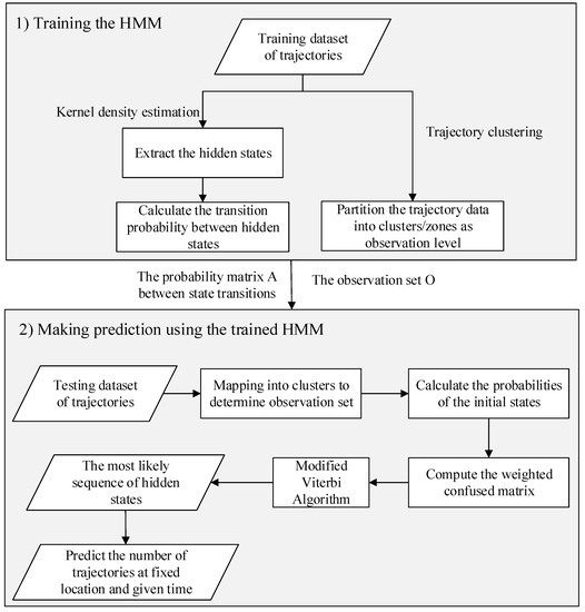
Figure 1.
The framework of the predictive model.
3.2. Model Methodology
The objective of the predictive model is to estimate the upcoming services of the vacant taxis near each fixed location corresponding to a hidden state in the HMM. The prediction can be derived by training the HMM as shown in Figure 1. The critical elements in training the HMM include the probability matrix of the transitions between states and the observation set . The probability matrix would be calculated using equation 1:
where represents the number of trajectories from state to state . In this approach, states and are extracted by a kernel density estimation conducted on the training dataset of trajectories. The other critical element, the observation set , would be generated by a trajectory clustering on the training dataset of trajectories. The prediction is described using the HMM as follows:
- Given a test trajectory, segment it at a given time interval, mark the current state at that time point, and then map it into corresponding clusters.
- Calculate the probabilities of the initial states using equation 2:where represents the number of trajectories near the fixed location corresponding to state at the initial time .
- Estimate the next state of the current trajectory at the next time interval, accounting for traffic conditions, such as the moving direction at the current time and the average speed at the same time interval.
- Calculate the weighted confusion matrix using equation 3:where is a coefficient that denotes the influence of state generated by cluster . We can calculate the coefficient using the difference between the location of state and the location of cluster by different impact factors including distance and speed. represents the number of trajectories observed by cluster at the hidden state .
- Calculate the partial probability of the hidden state at time using the following equation 4:
The maximum partial probability of the hidden state at time indicates that the likelihood of the next location near state is greater.
Here, we provide an example to demonstrate how to make predictions by exploiting the model. As shown in Figure 2, the set includes four hidden states, and the observation set includes a dozen elements. We calculated the initial probability matrix of states and the probability matrix of state transitions by using the historical trajectories based on the trained HMM. We partition the historical trajectories into different clusters at the observation level to analyze the influence of different contextual factors, such as the hour of the day and traffic conditions, belonging to each cluster in state . Therefore, we test which state sequences correspond to the fixed locations near where each trajectory passes, where the probability would reach its maximum. In other words, we expect to reach the maximum.
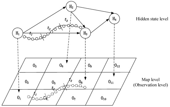
Figure 2.
An example of predictive modeling based on the hidden Markov model (HMM).
According to the Bayesian law, we can calculate the result by the following equation:
where the part corresponds to the confusion matrix B. More specifically, in this model, we use the weighted confusion matrix. The calculation steps are described as follows:
- Segment the test trajectory according to the given time interval. For instance, the test trajectory is segmented into three parts, corresponding to three time intervals,, and , in this example.
- Find out the corresponding cluster of each state. In this example, the four hidden states are observed to be the , , and clusters.
- Compute the weighted influence matrix of the clusters at the states according to the contextual factors.
- Compute the weighted confusion matrix using equation 3.
To predict the number of trajectories at a fixed location (state), we adopt the Viterbi algorithm and make a modification that estimates the next state at the next time interval before computing the partial probability of the hidden state to estimate the most likely sequence of hidden states. The most likely locations where this test trajectory passes include the fixed locations corresponding to the states ,, and . If a potential rider is waiting for a vacant taxi at some fixed location at a given time, such as between 7 and 8 am, we first calculate the current time period (we may suppose that the time period is every five minutes) of the test trajectories. Then, we calculate the possibility of each state in the next time interval. The maximum value denotes that the probability of state is the most likely location of the trajectory at the time period . For instance, if the current time interval is two, then we calculate the maximum value at the third period (after five minutes). According to the above calculation process, the result (3) means that the upcoming location is the fixed location of state after five minutes. In a similar fashion, if we want to calculate the most likely location after ten minutes, we can calculate the maximum value at the fourth period.
4. Experimental Results and Discussion
The experimental data used in this use case were from a 24-h dataset collected from 26 November to 30 November 2012, totaling over 37,326 trajectories generated from 1966 taxis. The time interval of the data collection is usually in the range of 30 s to 1 min. Delayed or missing data may occur depending on the quality of the GPS signal, and additional records were collected when the taxi load status changed. The testing data come from November 30, 2012. It was a Friday, and both business and shopping trips were on-going and recorded in large numbers. In this paper, the taxi trajectories during the morning peak period between 7: 00 and 9: 00 am, and the evening rush period between 5: 00 and 7: 00 pm, are tested.
4.1. Extration of Hidden States
Geographic events could occur anywhere spatially, but the probabilities of events occurring at different locations are different. Generally, the probabilities of events occurring in high-density regions are greater than the probabilities of those events occurring in more sparsely developed areas. In this paper, the potential taxi pickup hotspots represent those drop-off locations that are significantly concentrated in one place or in many places. How to determine the hidden states of the model is a crucial step before computing the probability transition matrix. We focus on discovering the popular spatial locations of taxi drop-offs and, thus, concentrate on estimating the spatial density of these drop-off events. We adopt the spatial kernel density method for extracting the prospective hotspots of taxi pickup locations.
Suppose that a location series is composed of drop-off events with locations ; the probability of drop-off events at location s would be estimated by the following spatial kernel density estimation (KDE) formula.
where represents the kernel and represents the spatial bandwidth. The spatial kernel function is a zero-mean probability density function, and the spatial bandwidth greatly affects the properties of the resulting density. A Gaussian function with a certain standard deviation is one of the most common and popular smoothing kernels. Here, we employ the Gaussian kernel to discover any high-density areas.
Forty eight thousand seven hundred and sixty eight drop-off points, which only cover the central portion of Beijing, were extracted for analysis. Moreover, only drop-off points with valid geocoded locations and time intervals were included. We derive the generalized areas of the hotspots with the KDE method, as mentioned above. Taxi drop-off points that were in the high-density areas were selected from the training dataset based on the locations of major business centers, shopping centers, universities and other traffic generating communities. Then, the corresponding trajectory origins were identified and extracted from the hotspots of taxi drop-off locations. As shown in Figure 3, there are 19 main high-density areas generated by KDE. The highest density areas are located around Liuliqiao, which is near to the Beijing West railway Station, and Zhongguancun, which is a popular computer and information science and technology production hub in Beijing. Most of these high-density areas could be potential locations corresponding to hidden states in our proposed predictive model.
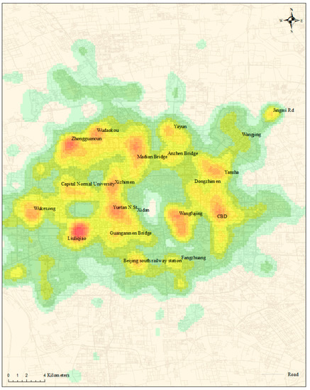
Figure 3.
Kernel density estimation (KDE) map of taxi drop-off locations within five days in Beijing.
4.2. Extrating Observation Set
To estimate the probability of hidden states, we build an observation set by partitioning the zones within the included range of taxi trajectories. Rather than a hard partitioning method, we adopt a fuzzy clustering approach that can deal with the uncertainty of samples belonging to different classifications. The Fuzzy C Means (FCM) algorithm is a clustering method based on an objective function. For a given dimensional data set , the algorithm is defined as follows [28]:
where represents the number of clusters, represents the number of data points, and represents the membership degree of data point belonging to the fuzzy cluster . In addition, represents the cluster centroid, and represents the weighting exponent, and also controls the fuzziness of the membership of each piece of data. As well as these, represents the Euclidean distance between and with plane coordinates. The FCM algorithm can divide the data set into different clusters by minimizing the objective function.
To obtain credible clustering results, the parameter of the FCM algorithm is set to 2, and the parameter for the iterative condition is . However, the fuzzy clustering algorithm is an unsupervised method, and the number of clusters must be selected beforehand. Here is set to 15, 20, and 25 to observe alternative clustering solutions. As a result, we obtain a collection of clusters, each of which contains a set of trajectory points with similar spatial features. However, different partitioning solutions lead to different prediction results. We describe the results in detail in the next section.
4.3. Predition Results and Discussion
To predict the probability of taking a vacant taxi, we perform the predictive model at major fixed locations where passengers expect to find vacant taxis at given times. We split the trajectory data into a training set and a testing set to implement our model. We use 1446 trajectories generated by 176 taxis as the testing dataset. According to the results of the KDE, as described above, and consistently with known popular commercial areas, we confirm 19 fixed locations corresponding to the hidden states in our predictive model. We mainly focus on the prediction results of the following 11 fixed locations: Xidan, Wangfujing, CBD, Dongzhimen, Xizhimen, Wukesong, Zhongguancun, Yayun, Wangjing, Yansha and Liuliqiao. Generally, taxi trip patterns are expected to be different in different zones according to the time of the day. For example, from 8 am to 9 am, taxi traffic may drop in business zones or near major subway stations because people are at work. However, taxi traffic may increase in residential or commercial zones after the evening peak. We performed experiments on the testing dataset at peak and off-peak times separately using the proposed model to compare the prediction results between different times of the day.
As mentioned above, we first build observation sets by partitioning trajectory data points into different zones within the covered range of taxi trajectories. Our prediction results are expected to be affected by different partitioning solutions. The partitioned zones can be seen as the observation set here as well. Before conducting the experimentation, we segment each testing trajectory at a given time interval, such as three minutes and five minutes, that can be adjusted according to actual traffic conditions. In our experimentation, we adopt five minutes as the temporal resolution of the trajectory segments. Here, we use the predicted accuracy ratio, dividing our predicted values by the actual values of vacant taxis, to compare the variance in the predicted accuracies between different partitions at each fixed location. Figure 4 shows the prediction accuracies during peak and off-peak times when the number of partitioning clusters is equal to 15, 20 and 25, respectively. From Figure 4a, we find that the prediction accuracy of the largest partition (number of clusters = 25) is higher than those of the partitions near areas such as Wangfujing, CBD and Dongzhimen. Specifically, the prediction accuracy reached one hundred percent near areas such as Dongzhimen and Zhongguancun. However, in other areas, such as Wangjing and Yansha, the prediction accuracy is far lower than that of the other partition results. The worst case is the prediction result near the area of Wukesong, as shown in Figure 4. For the smallest number of partitions (15), the worst prediction is found near the CBD. The prediction accuracy during the off-peak time, as shown in Figure 4b, is similar to those during the peak time under the different partition results. However, it is worth noting that a finer partition (number of clusters = 20) is more likely to make a better prediction in general, except for Xidan and Wangfujing. From the KDE map (Figure 3), it can be seen that Xidan and Wangfujing are lower-density areas. Therefore, we can conjecture that the training set could not provide a prediction model with enough prior experience for these clusters.
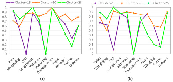
Figure 4.
Prediction accuracy at 11 fixed locations: (a) During peak times; (b) During off-peak times.
Considering the influence of the partitioning solutions, we set the number of clustering partitions equal to 20 in order to obtain better prediction results. To evaluate the performance of our predictive model, we compare the difference in the predicted accuracy between the peak and off-peak times in each fixed location, as shown in Figure 5. As expected, the time of the day appears to have different effects on the predictive accuracy of the model in different zones. From Figure 5, compared with the other areas, the predicted accuracy of the location around Zhongguancun achieves a maximum value of 100% during the AM and PM peak. In contrast, the predicted accuracy of the area around the CBD reaches a maximum value of 92.3 % during the off-peak. We also find from Figure 5 that during the peak times, the predictive accuracy of the pickup locations, which are more concentrated around the business areas of the city, is more likely to exceed the predicted accuracy during the rest of the day. For instance, the area around Zhongguancun is a major employment center where many high-tech corporations have major facilities. From the KDE map shown in Figure 3, we also find that this place is a high density trajectory area. As shown in Figure 6, the number of taxi drop-offs around this area during the evening rush hours exceeded that of the rest of the day. That is the possible reason why the predictive accuracy around Zhongguancun is very high during peak time. Whereas, the predictive accuracy of pickup locations in commercial areas, such as the CBD, during the off-peak time, is higher than the predictive accuracy during the peak time. In contrast to the predictive accuracy in Zhongguancun, the CBD is a financial, information, cultural and the business center area; therefore, taxi drop-offs around the area mainly focus on the off-peak time. In Figure 6, from 9 am to 12 am and 7 pm to 12 pm, we also see that the number of drop-offs around this CBD far exceeds those during the rest of day. Thus, the trained model on the historic trajectory data during the off-peak time would well support the prediction of our testing set.
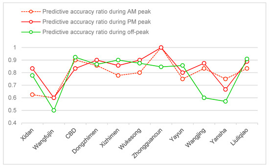
Figure 5.
Predictive accuracy ratio between peak and off-peak times.
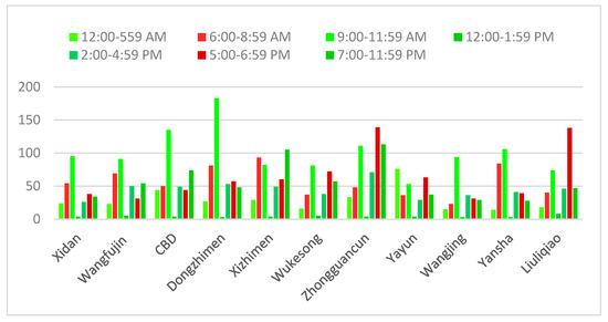
Figure 6.
The number of drop-offs during different time intervals within one day.
Finally, to visualize how well the predictive model performs, we map the observed points versus the predicted drop-off points for each taxi trajectory in the test set in Figure 7. In general, the predicted locations lie in close proximity to the observed values. For the evaluation accuracy of the predictive positions, Figure 8 details the statistical deviation between the predictive and the observed positions within a histogram of errors by distance bins. From Figure 8, we see that most of the predicted deviations fall within three bins: [100, 150], [150, 200] and [200, 250]. The trend line shows that the [150, 200] bin has the highest frequency according to the prediction results. The absolute deviation in the predicted location increases as the number of pickups increases, such as in Zhongguancun and Xizhimen. The absolute deviation is partially affected by the trajectory segmentation. The accuracy of the location prediction is improved by decreasing the granularity of the trajectory segmentation.
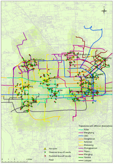
Figure 7.
Prediction results compared with the observed trajectories using the test data.
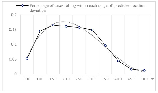
Figure 8.
Statistics of the deviations between the predicted and observed locations within each range.
5. Conclusions
Taxi transportation plays an important role in our daily life. Taking a taxi during peak time, parking problems and traffic congestion make finding vacant taxis more difficult. Special car services based on the Internet business model have also brought a big challenge to the taxi service industry. How to explore big taxi trajectory data to discover valuable information has been receiving increasing attention, as has building models for providing better taxi services.
In this paper we propose a model for predicting the upcoming services of vacant taxis in popular areas at a given time. Our predictive model is based on the HMM, along with the KDE method and the FCM algorithm, for extracting hidden states and partitioning traffic zones for building observation sets. Meanwhile, the predictive model combines contextual factors, including the time of day, traffic conditions and the number of partitioned traffic zones. Overall, our proposed modeling framework for predicting the upcoming services of vacant taxis in 11 popular areas in Beijing performed well. Our experimental analysis, including the predicted results and the location deviation analysis, supports our expectation about its predictive performance. On the basis of 176 taxis in Beijing, we find that the number of drop-offs is predicted with a 100% accurate in certain clusters during peak times of the day, and up to 92.3% in off-peak times. Because of the small number of historical trajectories in some popular areas like Wangfujing and Yansha, the average value of the predictive accuracy is pulled down to 77.8%, 83.2% and 78.4%, during AM peak, PM peak and off-peak respectively, in these areas. Even so, the predictive accuracy of most fixed locations exceeds 80%. Meanwhile, the proposed model demonstrates the ability of conducting location predictions, in which the average root mean square error between prediction and observation can be approximately 200 meters.
The predictive model in this study could be useful to city planners in projecting where to set taxi stands, to taxi dispatchers in resolving where to provide services and to taxi riders in figuring out where to find vacant taxis at different times of the day. With a recommender based on our modeling framework, passengers can get better service when taking a taxi because they know how many taxis will serve them in the next few minutes. Of course, the prediction model needs to be integrated to the taxi traffic management platform in order to satisfy the passengers’ demand in practice. While such implementation is beyond the scope of this research, we demonstrated the feasibility of such a system. We put forward a concept on how to leverage historical trajectory data and how to model taxi service dynamically using a large dataset of taxi trajectories.
However, there are limitations in the present state of the predictive model, which will mark the directions of future research. First, the prediction accuracy is affected by the training dataset. A larger dataset will be used in model training for providing better trained parameters in future work.
Second, the computational efficiency decreases with the increase of data volume. We will use a parallelized algorithm to deal with model training on a larger dataset. In addition, future work will extend current research in improving the predictive model and exploring more efficient approaches to extract observation sets.
Author Contributions
Conceptualization, Chunchun Hu; Methodology, Chunchun Hu and Jean-Claude Thill; Formal Analysis, Chunchun Hu; Investigation, Chunchun Hu; Data Curation, Chunchun Hu; Writing-Original Draft Preparation, Chunchun Hu; Writing-Review & Editing, Chunchun Hu and Jean-Claude Thill; Visualization, Chunchun Hu; Supervision, Jean-Claude Thill; Project Administration, Chunchun Hu; Funding Acquisition, Chunchun Hu.
Funding
This research was funded by National Key R&D Program of China under grant number 2018YFC0809100; The Fundamental Research Funds for Central Universities under grant number 2042017kf0224.
Conflicts of Interest
The authors declare no conflict of interest.
References
- Beijing Transport Institute. Beijing Transportation Development Annual Report in 2018. Available online: http://www.bjtrc.org.cn/List/index/cid/7.html (accessed on 10 March 2019).
- Soares Júnior, A.; Moreno, B.N.; Times, V.C.; Matwin, S.; Cabral, L.D.A.F. GRASP-UTS: An algorithm for unsupervised trajectory segmentation. Int. J. Geogr. Inf. Sci. 2015, 29, 46–68. [Google Scholar] [CrossRef]
- Alewijnse, S.; Buchin, K.; Buchin, M.; Kölzsch, A.; Kruckenberg, H.; Westenberg, M.A. A framework for trajectory segmentation by stable criteria. In Proceedings of the 22nd ACM SIGSPATIAL International Conference on Advances in Geographic Information Systems (ACM), Dallas, TX, USA, 4–7 November 2014. [Google Scholar]
- Hwang, S.; VanDeMark, C.; Dhatt, N.; Yalla, S.V.; Crews, R.T. Segmenting human trajectory data by movement states while addressing signal loss and signal noise. Int. J. Geogr. Inf. Sci. 2018, 32, 1391–1412. [Google Scholar] [CrossRef]
- Nogueira, T.P.; Braga, R.B.; De Oliveira, C.T.; Martin, H. FrameSTEP: A framework for annotating semantic trajectories based on episodes. Expert Syst. Appl. 2018, 92, 533–545. [Google Scholar] [CrossRef]
- Junior, A.S.; Times, V.C.; Renso, C.; Matwin, S.; Cabral, L.A. A semi-supervised approach for the semantic segmentation of trajectories. In Proceedings of the 2018 19th IEEE International Conference on Mobile Data Management (MDM), Aalborg, Denmark, 25–28 June 2018. [Google Scholar]
- Zhou, Z.; Dou, W.; Jia, G.; Hu, C.; Xu, X.; Wu, X.; Pan, J. A method for real-time trajectory monitoring to improve taxi service using GPS big data. Inf. Manag. 2016, 53, 964–977. [Google Scholar] [CrossRef]
- Cui, J.; Liu, F.; Janssens, D.; An, S.; Wets, G.; Cools, M. Detecting urban road network accessibility problems using taxi GPS data. J. Transp. Geogr. 2016, 51, 147–157. [Google Scholar] [CrossRef]
- Gong, L.; Liu, X.; Wu, L.; Liu, Y. Inferring trip purposes and uncovering travel patterns from taxi trajectory data. Cartogr. Geogr. Inf. Sci. 2016, 43, 103–114. [Google Scholar] [CrossRef]
- Mao, F.; Ji, M.H.; Liu, T. Mining spatiotemporal patterns of urban dwellers from taxi trajectory data. Front. Earth Sci. 2016, 10, 205–221. [Google Scholar] [CrossRef]
- Zhao, P.X.; Qin, K.; Ye, X.Y.; Wang, Y.L.; Chen, Y.X. A trajectory clustering approach based on decision graph and data field for detecting hotspots. Int. J. Geogr. Inf. Sci. 2017, 31, 1101–1127. [Google Scholar] [CrossRef]
- Tang, L.; Yang, X.; Kan, Z.; Li, Q. Lane-level road information mining from vehicle GPS trajectories based on naïve bayesian classification. ISPRS Int. J. Geo Inf. 2015, 4, 2660–2680. [Google Scholar] [CrossRef]
- Chen, C.; Zhang, D.; Li, N.; Zhou, Z.-H. B-planner: Planning bidirectional night bus routes using large-scale taxi GPS traces. IEEE Trans. Intell. Transp. Syst. 2014, 15, 1451–1465. [Google Scholar] [CrossRef]
- Zhou, Y.; Fang, Z.; Thill, J.-C.; Li, Q.; Li, Y. Functionally critical locations in an urban transportation network: Identification and space–time analysis using taxi trajectories. Comput. Environ. Urban Syst. 2015, 52, 34–47. [Google Scholar] [CrossRef]
- Chen, M.; Liu, Y.; Yu, X. Predicting next locations with object clustering and trajectory clustering. Comput. Vis. ACCV 2018 2015, 9078, 344–356. [Google Scholar]
- Qiao, S.J.; Shen, D.Y.; Wang, X.T.; Han, N.; Zhu, W. A self-adaptive parameter selection trajectory prediction approach via hidden Markov models. IEEE Trans. Intel. Transp. Syst. 2015, 16, 284–296. [Google Scholar] [CrossRef]
- Chen, M.; Yu, X.H.; Liu, Y. Ming moving patterns for predicting next location. Inf. Syst. 2015, 54, 156–168. [Google Scholar] [CrossRef]
- Yuan, N.J.; Zheng, Y.; Zhang, L.; Xie, X. T-finder: A recommender system for finding passengers and vacant taxis. IEEE Trans. Knowl. Data Eng. 2013, 25, 2390–2403. [Google Scholar] [CrossRef]
- Qiu, Z.; Li, H.Y.; Hong, S.D. Finding vacant taxis using large scale GPS traces. Lect. Notes Comput. Sci. 2014, 8485, 793–804. [Google Scholar]
- Hou, Y.; Li, X.; Zhao, Y.; Jia, X.; Sadek, A.W.; Hulme, K.; Qiao, C. Towards efficient vacant taxis cruising guidance. In Proceedings of the IEEE Global Communications Conference, Atlanta, GA, USA, 9–13 December 2013. [Google Scholar]
- Xu, X.; Zhou, J.Y.; Liu, Y.; Xu, Z.Z.; Zha, X.W. Taxi-RS: Taxi-hunting recommendation system based on taxi GPS data. IEEE Trans. Intell. Transp. Syst. 2015, 16, 1–12. [Google Scholar] [CrossRef]
- Zhang, D.; Sun, L.; Li, B.; Chen, C.; Pan, G.; Li, S.; Wu, Z. Understanding taxi service strategies from taxi GPS traces. IEEE Trans. Intell. Transp. Syst. 2015, 16, 123–135. [Google Scholar] [CrossRef]
- Wong, R.; Szeto, W.; Wong, S. Bi-level decisions of vacant taxi drivers traveling towards taxi stands in customer-search: Modeling methodology and policy implications. Transp. Policy 2014, 33, 73–81. [Google Scholar] [CrossRef]
- Tang, J.; Jiang, H.; Li, Z.; Liu, F.; Wang, Y. A two-layer model for taxi customer searching behaviors using GPS trajectory data. IEEE Trans. Intell. Transp. Syst. 2016, 17, 1–7. [Google Scholar] [CrossRef]
- Phithakkitnukoon, S.; Veloso, M.; Bento, C.; Biderman, A.; Ratti, C. Taxi-aware map: Identifying and predicting vacant taxis in the city. Trans. Rough Sets VII 2010, 6439, 86–95. [Google Scholar]
- Moreira-Matias, L.; Gama, J.; Ferreira, M.; Mendes-Moreira, J.; Damas, L. Predicting taxi–passenger demand using streaming data. IEEE Trans. Intell. Transp. Syst. 2013, 14, 1393–1402. [Google Scholar] [CrossRef]
- Microsoft Research. Inferring Taxi Status Using GPS Trajectories. Available online: https://www.microsoft.com/en-us/research/wp-content/uploads/2016/02/MSRA-TR_taxi_status.pdf (accessed on 2 May 2018).
- Bezdek, J.C. Pattern Recognition with Fuzzy Objective Function Algorithms; Plenum Press: New York, NY, USA, 1981. [Google Scholar]


© 2019 by the authors. Licensee MDPI, Basel, Switzerland. This article is an open access article distributed under the terms and conditions of the Creative Commons Attribution (CC BY) license (http://creativecommons.org/licenses/by/4.0/).