Article

Landslide Susceptibility Assessment Using an Optimized Group Method of Data Handling Model

1
Deputy Chairman of the State Committee on Geology and Mineral Resources, 11, T. Shevchenko, Tashkent 100060, Uzbekistan
2
Geoscience Platform Division, Korea Institute of Geoscience and Mineral Resources (KIGAM), 124, Gwahak-ro, Yuseong-gu, Daejeon 34132, Korea
3
Department of Geophysical Exploration, Korea University of Science and Technology, 217 Gajeong-ro Yuseong-gu, Daejeon 34113, Korea
4
Center for Environmental Data Strategy, Korea Environment Institute (KEI), 370 Sicheong-daero, Sejong-si 30147, Korea
*
Author to whom correspondence should be addressed.
ISPRS Int. J. Geo-Inf. 2020, 9(10), 566; https://doi.org/10.3390/ijgi9100566
Submission received: 19 August 2020 / Revised: 21 September 2020 / Accepted: 28 September 2020 / Published: 29 September 2020
(This article belongs to the Special Issue Multi-Hazard Spatial Modelling and Mapping)

Abstract

:
Landslides can cause considerable loss of life and damage to property, and are among the most frequent natural hazards worldwide. One of the most fundamental and simple approaches to reduce damage is to prepare a landslide hazard map. Accurate prediction of areas highly prone to future landslides is important for decision-making. In the present study, for the first time, the group method of data handling (GMDH) was used to generate landslide susceptibility map for a specific region in Uzbekistan. First, 210 landslide locations were identified by field survey and then divided randomly into model training and model validation datasets (70% and 30%, respectively). Data on nine conditioning factors, i.e., altitude, slope, aspect, topographic wetness index (TWI), length of slope (LS), valley depth, distance from roads, distance from rivers, and geology, were collected. Finally, the maps were validated using the testing dataset and receiver operating characteristic (ROC) curve analysis. The findings showed that the “optimized” GMDH model (i.e., using the gray wolf optimizer [GWO]) performed better than the standalone GMDH model, during both the training and testing phase. The accuracy of the GMDH–GWO model in the training and testing phases was 94% and 90%, compared to 85% and 82%, respectively, for the standard GMDH model. According to the GMDH–GWO model, the study area included very low, low, moderate, high, and very high landslide susceptibility areas, with proportions of 14.89%, 10.57%, 15.00%, 35.12%, and 24.43%, respectively.

1. Introduction

Landslides are one of the most widespread and common natural hazards in hilly and mountainous areas [1], where they can cause loss of life, property damage, and severe damage to the environment and foundations of roads and highways. Models predicting landslide occurrence have attracted considerable attention, as landslides have increased in many parts of the world due to both climate change and anthropogenic activities. Although more high-intensity and short-duration rainfall (heavy rainfall) is occurring, thus triggering more landslides, the pressure exerted by the urbanization of mountain areas, the cutting of trees to construct homes, and poor watershed management are the most important reasons for the increase in landslides [2]. The Centre for Research on the Epidemiology of Disasters (CRED) declared that 17% of the damage caused by natural disasters is due to landslides. Moreover, many researchers believe that this proportion will increase due to additional pressure on the environment from population growth, and to the effects of climate change [3].
One of the main approaches to reducing damage from landslide disasters is to determine landslide-prone areas. To achieve this, the first step is to gather information about landslide occurrences and the conditioning factors. Landsliding is a complex process associated with various geo-environmental factors, such as slope, altitude, geology, lithological properties, and soil type [4,5], as well as rainfall and anthropogenic activities (as triggering events) [6]. Several approaches have been developed and implemented for landslide predictions, based on the relationship between landslide conditioning factors and historical data and exploiting advances in remote sensing and geographic information systems (GIS). These methods can be classified into four main types: bivariate, multivariate, multi-criteria decision-making (MCDM), and artificial intelligence (AI) algorithms.
Bivariate and multivariate models have been used all over the world for natural hazard susceptibility assessment. The frequency ratio (FR) [4], weight of evidence (WoE) [6], evidential belief function (EBF) [7], Shannon entropy (SE) [8], and logistic regression [9] techniques are well-known. However, although these methods are simple to implement and produce data that are easy to interpret, the data have high uncertainty because non-event locations are not considered in the modeling process; this leads to exaggeration of the extent of the landslide-prone area.
The MCDM approach subsumes many methods, such as analytical hierarchy processes (AHPs) [10], analytical network processes (ANPs) [11], Viekriterijumsko Kompromisno Rangiranje (VIKOR) [12] and the technique for order of preference by similarity to ideal solution (TOPSIS) [13], among others. Although MCDM has been applied successfully in many scientific fields, including for natural hazard susceptibility assessment, its utility is diminished by uncertainty due to reliance on expert opinion [14]. Khosravi et al. [15] compared the results of TOPSIS and VIKOR with those of AI models, with the latter proving more practical and reliable.
Recently, AI algorithms have attracted the attention of researchers all over the world due to their flexibility, good performance, and ability to handle large datasets [16,17]. The artificial neural network (ANN) is the most widely used type of AI algorithm in geoscience, especially for landslide modeling. [18] used an ANN model for landslide modeling in Korea. A change detection technique was applied to Korea Multipurpose Satellite (KOMPSAT-1) electro-optical camera (EOC) images to determine landslide locations. The ANN was able to identify landslide-prone areas with an accuracy of 82.72%. Pascale et al. [19] produced a map of highly landslide-prone areas in southern Italy using an ANN model. Shahri et al. [20] applied an ANN algorithm for landslide susceptibility mapping in southern Sweden and reported that the ANN was a cost-effective tool for land management and landslide hazard mitigation. However, the ANN approach has some drawbacks, such as relatively poor prediction power and generalizability, and low convergence speed [21,22]; thus, ANN algorithms combined with fuzzy logic models with the adaptive neuro-fuzzy inference system (ANFIS) have been generated. The ANFIS shows better performance than ANN models and has been applied successfully to landslide hazard modeling [23]. Dehnavi et al. [24] reported reasonable predictive power of the ANFIS for landslide modeling in Iran. Polykretis et al. [25] applied the ANFIS to generate a landslide susceptibility map for a hilly Mediterranean area; the accuracy was reported as 0.70–0.90, indicating fair to very good model performance. They also found that the performance depended strongly on the weights and types of membership functions. Bui et al. [26] reported similar findings, and mentioned that the membership functions were the main source of uncertainty. The support vector machine (SVM) is another powerful AI model that has been widely applied for generating landslide susceptibility maps worldwide. Ballabio and Sterlacchini [27] applied the SVM for landslide modeling at Lombardy, northern Italy; the model was robust and reliable. Lee et al. [28] applied the SVM for landslide modeling and map generation in Gangwon Province, Korea; the model accuracy for areas in PyeongChang and Inje was 81.36% and 77.49%, respectively. It should be noted that the SVM is sensitive to hyperparameters, and the requirement to select the best kernel reduces its applicability.
Another type of AI model, the data-mining model, has been used widely for natural hazard susceptibility assessment, and especially for landslide hazard modeling. Dou et al. [29] used a random forest (RF) model for landslide susceptibility mapping on the volcanic island of Izu Oshima, Japan. Their RF model had high predictive power in landslide hazard-prone areas. Chen at al. (2018) applied kernel logistic regression for landslide modeling in Shangnan County, China; their model showed reasonable accuracy. Pham et al. [30] compared the predictive accuracy of RF, logistic model tree (LMT), best first decision tree (BFDT), and classification and regression tree (CART) landslide models in India. They found that the RF model outperformed the other models. Although these methods have been applied successfully for landslide modeling, they have lower performance than traditional approaches, such as the ANFIS and SVM, etc. Pham et al. [31] compared the performance of naïve Bayes tree (NBT), Bayes network (BN), naïve Bayes (NB), and decision table naïve Bayes (DTNB) data-mining algorithms with the SVM for landslide susceptibility mapping in India, and concluded that the SVM outperformed the algorithms. Honge et al. [32] used hybrid algorithm of AdaBoost, Bagging and Rotation Forest with decision tree algorithm for landslide susceptibility mapping at China. They declared that hybrid algorithm of Rotation Forest had a higher prediction power than AdaBoost, and Bagging models. Bui et al. [33] used four hybrid models of Adaboost, bagging, rotation forest, and random subspace with SVM model and finally stated that random subspace model outperform of other models. Napoli et al. [34] applied hybrid algorithm of artificial neural network, generalized boosting model and maximum entropy for landslide susceptibility mapping at Italy and finally stated that hybridization improved the prediction power of the standalone models. Table 1 summarizes the literature review. Ngo et al. [17] applied deep learning algorithm of convolutional neural networks (CNN), and recurrent neural networks (RNN), to future landslide occurrences prediction at national scale of Iran. They finally stated that both algorithms have the high accuracy, while RNN model is more accurate than CNN.
The group method of data handling (GMDH) is a neuron model that has been applied successfully for time-series prediction, but not for natural hazard susceptibility assessment (especially landslide modeling). Ebtehaj et al. [37] applied the GMDH for discharge coefficient (Cd) prediction of side weirs; the GMDH showed very good predictive performance. Shaghaghi et al. [38] used the GMDH for stable channel geometry analysis and stated that the GMDH model outperformed other empirical equations.
The main objective of the current study was to investigate the effectiveness of the GMDH for landslide susceptibility mapping. The fact that the GMDH has not yet been applied for natural hazard susceptibility assessment was the motivation for this study. The GMDH is a powerful neuron model; similar to other neuron models, it suffers from the determination of weights of membership function and other operators. Thus, in the present study, the predictive performance of a hybrid GMDH/gray wolf optimizer (GWO) was also examined.

2. Study Area

The Bostanlyk District is located in the Tashkent region of Uzbekistan between long 66′ 45 E to 66′ 12 E and lat 38′ 45 N to 38′ 60 N, which is characterized by relatively uniform relief (mainly hills, mountains, and other areas of elevation). Within the Bostanlyk District, the Tekstilsik landslide is a large, recent landslide area located on the left bank of the Chirchik river basin, within the northern part of the Alizar anticline [which is characterized by Cretaceous clays and siltstones at the intersection of the “Alizar uplift” (with northwest strike) and the Karankul fault (with latitudinal strike; Figure 1)]. The landslide has a volume of 22.5 × 10⁶ m3. Landslide displacement affects the top part (1.4–1.5 km) of the slope. The landslide area is 500 m wide in the upper zone and 250–300 m wide in the lower zone. The elevation at the fault wall of the upper point of landslide initiation is at absolute marks 1018–1108 m. The separation location of the lower point of landslide initiation is at 850–790 m. The landslide area has experienced several earthquakes and some landslides triggered by them. The territory is a part of tectonic active structure of the lithosphere of Western Tian-Shan and earthquakes with the magnitude of 9 (on Richter scale) will occur. The 20-year average precipitation (rainfall) is 550–650 mm (range: 300–900 mm). The temperature in the area ranges from 40 °C in July to −5 °C in January (average = 13 °C). Groundwater monitoring at Tekstilsik landslide area started in 1980. According to the results, the groundwater level on slopes disturbed by displacement ranges from 2.3 to 5.5 m; in undisturbed areas, the groundwater is much deeper (range: 16.42–19.16 m).
In the study area, from top to bottom, there stands out an undulating watershed of mountain rivers, which formation was completed via tectonic-erosion cycles. The slopes of the terrace surfaces are not exceeded 8–10°, dividing their slopes have a steepness of 12–15°. In the central part, the surface of these terraces and slopes are complicated by large cirques formed by landslide occurrences.
Within the landslide area, the upper generation, the lower and the landslide toe are distinguished. In turn, the upper generation is divided into an upper stage and a lower one which a landslide depression separating them. The fault wall of the upper generation (elevation 1018–1108 m) is confined to the terrace ledge, the landslide depression and the lower step to the terrace surface (1020–900 m). The toe of the landslide falls at 790–850 m. Modern landslide displacements can be traced down the slope 1.4–1.5 km, 500 m wide in the upper and 250–300 m in the lower zones. The peculiarity of the structure is its division into two parts with the formation of a graben along the line, due to the uplift. The influence of natural factors on the dynamics of a landslide (geological, morphological, physical, artificial) is associated with the confinement to the uplift zone, the rise in the level of pressurized underground waters of the complex aquiferous of Cretaceous beddings. The reasons that play a trigger role are the simultaneous waterlogging of rocks from melted snow, precipitation and groundwater.
In fact, the Tekstilsik landslide is divided into two parts by graben formation due to the Alizar uplift. The landslide area is composed of 20–30-m-thick loess rock in the middle/upper part, but the thickness decreases to 5 m in the lower part.
Clay loams are separated by interbedded Cretaceous clays, siltstones, sandstones, and gravelites. The thickness of the layers varies from 2–4 m, which are at least 100 m deep. The water-bearing horizon is in the range of 25–45 m. Groundwater from springs at the base of scarps flows down the graben and slope, and forms small lakes and swamps. The groundwater emanates from loamy Quaternary sediments at a depth of 0.4–26.0 m, as springs with flow rates of 0.1–0.5 l/s in both the upper and lower areas. Pressurized interlayer groundwater emanates from Cretaceous sediments underlying the Quaternary sediments.
It is worth mentioning that the Tekstilsik landslide is located in the northern part of Uzbekistan on the left bank of the Chirchik river basin; the second zone is located in the southern part of the Aksu–Tankazdarya river basin, and occupies the middle and upper parts of the river valley. The area of the zone is about 160–170 km2. Paleozoic rocks are predominant in the upper reaches, while Meso–Cenozoic sandy–clayey rocks (mostly Cretaceous) are well-represented in the middle part of the valley. These deposits are overlaid by 5–20-m-thick loams.
The study area is favorable for the formation of block landslides because of the monoclinal bedding of Meso–Cenozoic rocks, which also contain several independent aquifers. Interstratal karst provides favorable conditions for water saturation of the overlying loams and underlying clays, leading to the formation of large landslides. Landslides are most active on the right bank of the Akdarya and the left bank of the Tamshushdarya in the villages of Miraki, Nondek, and Tamshush, where Meso–Cenozoic rocks are bedded in a manner consistent with the slope. Within these villages, block landslides may occur; loams and underlying sandy–clayey deposits extending to a depth of 20–30 m are involved in the landslides, the volumes of which can reach tens of millions of cubic meters (e.g., the Nondek landslide on 04/24/92: volume = 22 million m3). The landslides move relatively slowly as elastic flows.
The Tankazdarya landslide zone occupies the middle and upper parts of the river valley. Geologically, the zone is confined to the front part of the Lyangar thrust fault. The landslides are most frequent on the limbs of anticlinal structures composed of Cretaceous–Neogene rocks. As the area is characterized by cuesta relief, the landslides are usually displaced along several sliding surfaces and are large in scale (Table 2 and Figure 2).

3. Data and Method

3.1. Historical Landslide Data

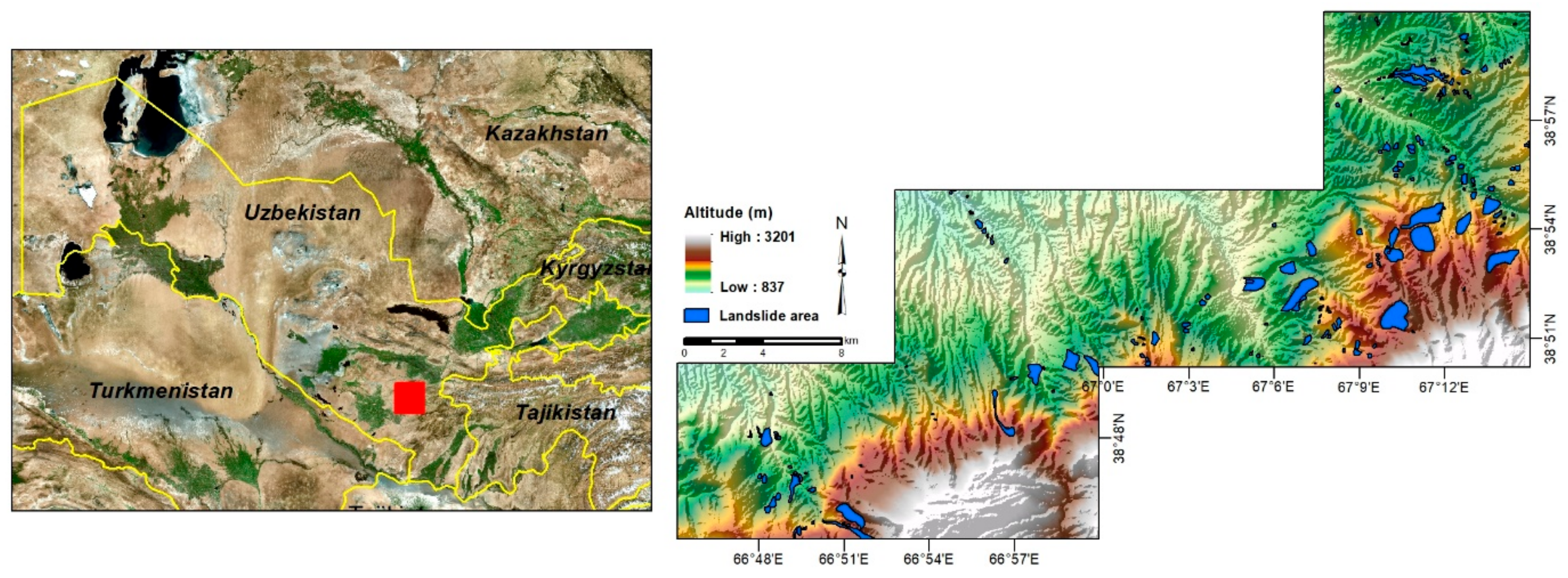
The first step in natural hazard modeling, such as landslide susceptibility mapping, is collecting and compiling a dataset of historical events. The aim is to identify relationships between landslide historical data and a geo-environmental dataset, and then to use these relationships to formulate and predict future landslide occurrences. Thus, the accuracy and quality of the historical dataset used has a significant impact on the prediction results [39]. In the present study, 210 polygons were initially identified on aerial photographs as the triggering area of the landslide and subsequently confirmed through extensive field surveys (Figure 2). It means that their location was detected much easier in the field surveys. Their locations were recorded using GPS handhold. Afterwards, the center of gravity of each polygon was considered as the landslide location. As landslide susceptibility assessment uses a binary modeling approach, except for 210-landslide location, the same number of locations from those areas in which landslides had not occurred were generated randomly in ArcGIS 10.2 (Esri, Redlands, CA, USA). Shirzadi et al. [9] stated that the dataset should be divided into training and model validation datasets; the data used in this study were divided thusly (70% and 30%, respectively). Both the landslide and non-landslide locations were divided into two parts (70% and 30% of the data). The 70% portions of the landslide and non-landslide locations were combined and used as the model training dataset; the 30% portions were integrated to form the testing dataset for model validation.

3.2. Conditioning Factors

For comprehensive landslide modeling, we determined the most important landslide conditioning factors. The following nine conditioning factors were identified via a literature review, and according to the characteristics of the study area [4]: altitude [30], slope degree [36], slope aspect [5], topographic wetness index (TWI) [40], length of slope (LS) [41], valley depth [28], distance from roads [42], distance from rivers [30], and geology [43].
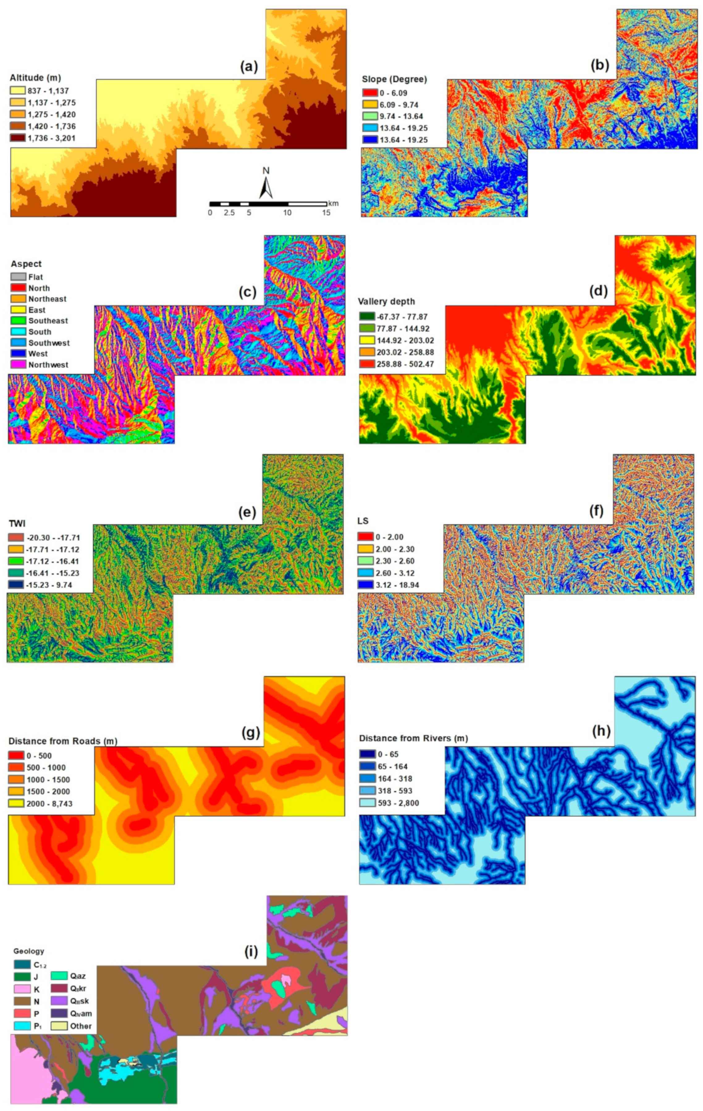
First, a digital elevation model (DEM) was devised with a pixel size of 30 × 30 m, which was downloaded from USGS Earth Explorer website, and altitude, slope degree, slope aspect, and LS data were derived directly from the DEM using ArcGIS 10.2 (Esri, Redlands, CA, USA). Altitude has an indirect effect on landslide likelihood through its major impact on rainfall, vegetation cover, soil thickness, and tectonics, all of which are important factors in landslide modeling [42,43,44]. These factors were also modeled using ArcGIS 10.2 (Figure 3a). Slope degree affects the probability of landslide occurrence via shear stress and gravitational acceleration, which tend to move mass down a hillslope if the soil layer is sufficiently thick: steeper slopes increase the probability of landslide occurrence. A slope map of the study area is shown in Figure 3b. Soil wetness varies by slope aspect, attributable to the effect of solar radiation, as do hydrological processes such as runoff, infiltration, evaporation, etc., which also affect the probability of landslide occurrence. According to the literature, the south aspect of the study area is wetter such that the landslide probability is greater. A slope aspect map is presented in Figure 3c. Valley depth (difference in elevation between the valley and upstream ridge) affects slope stability and thus the probability of landslide occurrence [45]. We calculated valley depth based on the method of Menking et al. [46], as shown in Figure 3d. The TWI is a major factor which indicates the soil moisture on slopes and, by extension, on infiltration, runoff generation and ultimately landslide probability [30]. Our DEM was used to derive the TWI via SAGA–GIS software (http://saga-gis.org) (Figure 3e).
The LS also has a major effect on landslide probability: longer LS promotes landslide occurrence, the longer LS, the more gravitational acceleration can affect detach part of the hillslope [41]. This factor was calculated from our DEM using SAGA–GIS software (Figure 3f). According to the literature, most of the landslides occurred near the road network system [40]. Road construction can cause a discontinuity in the soil on a hillslope, making it more prone to landslides. The distance between landslides and roads was calculated based on the road network layer using ArcGIS 10.2 (Figure 3g). When a landslide site is closer to a river, soil moisture is higher. Therefore, the hillslope is heavier, which makes it more prone to landslides. Pham et al. [30] reported that about 65% of the landslides in Uttarakhand, India, were close to a river. The river layer in our study was based on the river network layer in ArcGIS 10.2 and is shown in Figure 3h. Lithological formations differ in structure and strength, and greatly affect the likelihood of soil discontinuity and landslide occurrence [47]. Nguyen et al. [41] stated that the geology and slope degree have a major effect on landslide probability. The lithological units in the study are shown in Figure 3i. All conditioning factors prepared in proper classes shown in Figure 3 and Table 3.
Finally, the training data were overlaid with all of the conditioning factors and used for modeling. The data were converted into an Excel file (Microsoft Corp., Redmond, WA, USA) for use in MATLAB (MathWorks, Natick, MA, USA).

3.3. Method

3.3.1. Group Method of Data Handling (GMDH)

The GMDH, which was developed by Ivakhnenko [48], can be employed to solve highly nonlinear problems, and for multiple-input to single-output systems because of its heuristic self-organizing characteristics [49]. The GMDH can select input variables, the number of neurons, and the number of layers to optimize the model. The GMDH involves different pairs of neurons, which are connected through a quadratic polynomial function to generate new neurons in the next layer. For a given input vector x = { x i 1 , x i 2 , x i 3 , , x i n } , the mathematical relationship between the observation input data and output variables can be computed by the Volterra–Kolmogorov–Gabor function, as follows:
y ^ ( x 1 , , x n ) = a 0 + i = 1 n a i x i + i = 1 n j = 1 n a i j x i x j + i = 1 n j = 1 n k = 1 n a i j k x i x j x k +
where y ^ represents the forecasted value and A ( a 1 , a 2 , , a n ) denotes the undetermined weighting coefficients, which can be calculated via regression by minimizing the square of the difference between the forecasted values and actual output [50]. Additional explanation of the GMDH and its equations is provided elsewhere [51,52,53,54].
To determine the optimum number of hidden layers, which each contain a set of neurons, the GMDH can be combined with metaheuristic algorithms, such as the GWO.

3.3.2. Gray Wolf Optimizer (GWO)

The meta-heuristic GWO was proposed by [55]. The GWO is based on the leadership hierarchy and hunting strategy of gray wolves. Generally, wolves in a pack are divided into four types with specific roles: alpha ( α ), beta ( β ), delta ( δ ), and omega ( ω ). The alpha wolf (most dominant) is the leader of the pack. The omega wolves (least dominant), which play a significant role in preventing infighting, are at the bottom of the social pyramid [56,57]. The hunting behavior of gray wolves encompasses encircling, hunting, and attacking the prey [58].
When mathematically modeling the social hierarchy of wolves, the three best solutions in terms of the fitness function value are called α , β , and δ , respectively; all other solutions are considered as ω . The encircling process can be described using the following equations:
X ( t + 1 ) = X p ( t ) A . C . X p ( t ) X ( t ) A = 2 a . r 1 a a n d C = 2 . r 2
where X p and X represent the position vectors of the prey and a gray wolf, A and C denote coefficient vectors, and t indicates the current iteration. r 1 and r 2 are random vectors that take values between 0 and 1, and a changes linearly from 2 to 0 during each iteration [59].
After encircling the prey, the hunting process is conducted by wolves α , β , and δ . Given their superior knowledge of the likely position of the prey, other wolves modify their positions accordingly, as described by the following formulae [36]:
D α = C 1 . X α X , D β = C 2 . X β X , D δ = C 3 . X δ X
X 1 = X α A 1 . D α , X 2 = X β A 2 . D β , X 3 = X δ A 3 . D δ
X ( t + 1 ) = X 1 + X 2 + X 3 3
Finally, the prey will be attacked when A 1 , and algorithm exploitation will be improved. When, A 1 exploration is emphasized such that the wolves find better prey [60,61].

3.4. Model Validation

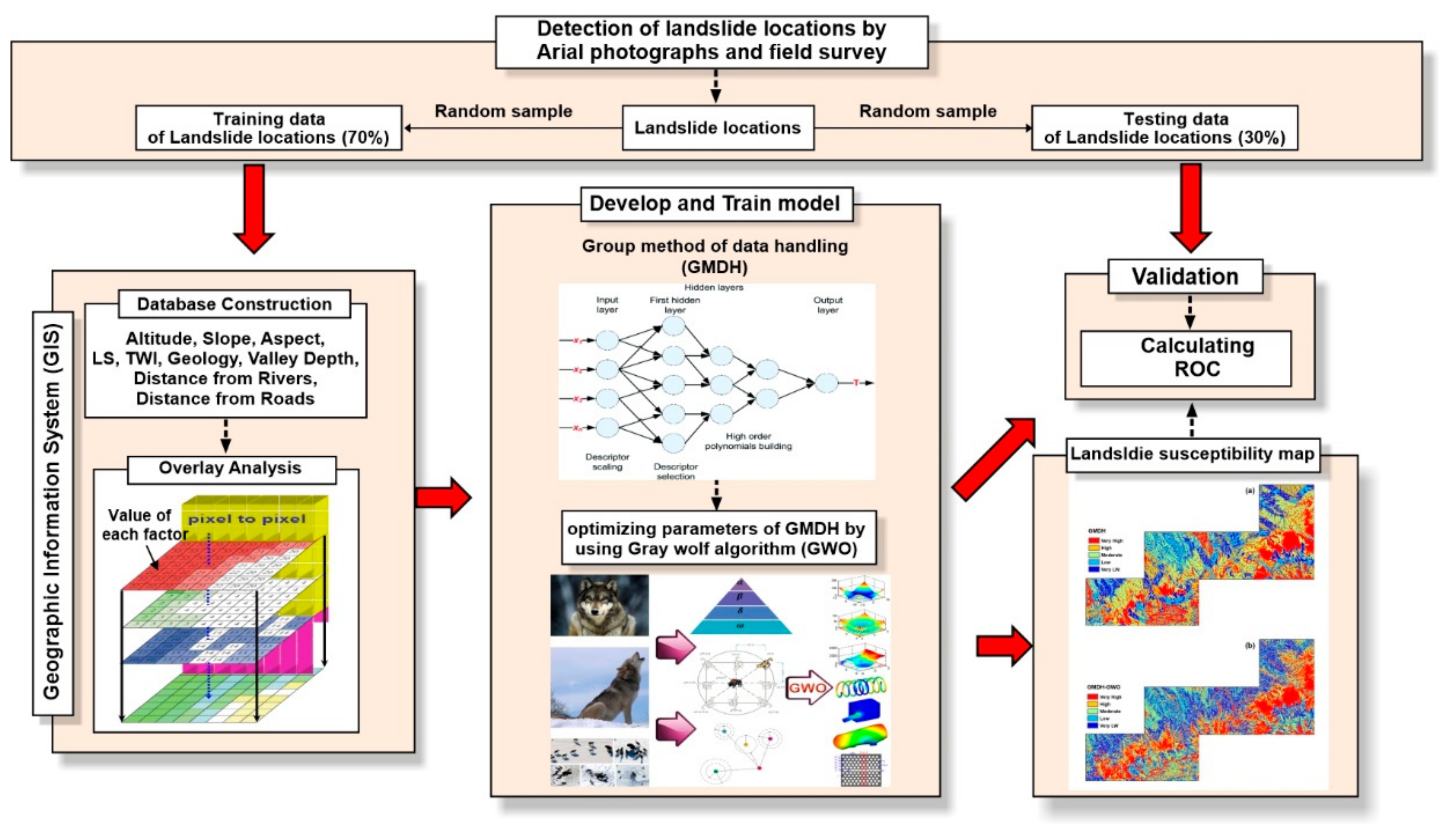
Model validation is one of the most important steps in the modeling process to ensure reliability [62]. The present study used receiver operating characteristic (ROC) curve analysis, which is the most popular method for model validation [4,8]. ROC curve analysis quantifies model performance according to the area under the ROC curve (AUC); this is the main advantage of this approach [63]. The AUC varies between 0.5 and 1; and ideal model has an AUC of 1 [4]. Figure 4 represents an overview of employing the proposed models to generate the landslide susceptibility maps.

4. Results and Discussion

4.1. Impact of Conditioning Factor Subclasses on Landslide Probability

In this section, the FR was used to determine the impact of the conditioning factor subclasses on landslide probability in the study area (Table 3). The results showed that the probability of landslide occurrence increased with altitude until 1736 m; it decreased thereafter. The probability of landslide occurrence was highest at an altitude of 1275–1420 m. Among the slope aspects, landslide probability was highest with southwest and south aspects. Landslide probability was also greater with a longer LS (3.12–18.94 m). Distances from the landslide area to the river below 590 m also promoted landslide occurrence (FR > 1) relative to distance larger than 590 m. Greater distance of the landslide area from a road, i.e., more than 2365 m, was associated with lower landslide likelihood compared to distances below 2365 m. Regarding slope degree, the landslide occurrence would be higher for moderate slopes. Thus, only 6–13° slopes in the study area promoted landslide occurrence. Finally, landslide occurrence probability was higher when valley depth was lower.

4.2. Landslide Susceptibility Maps

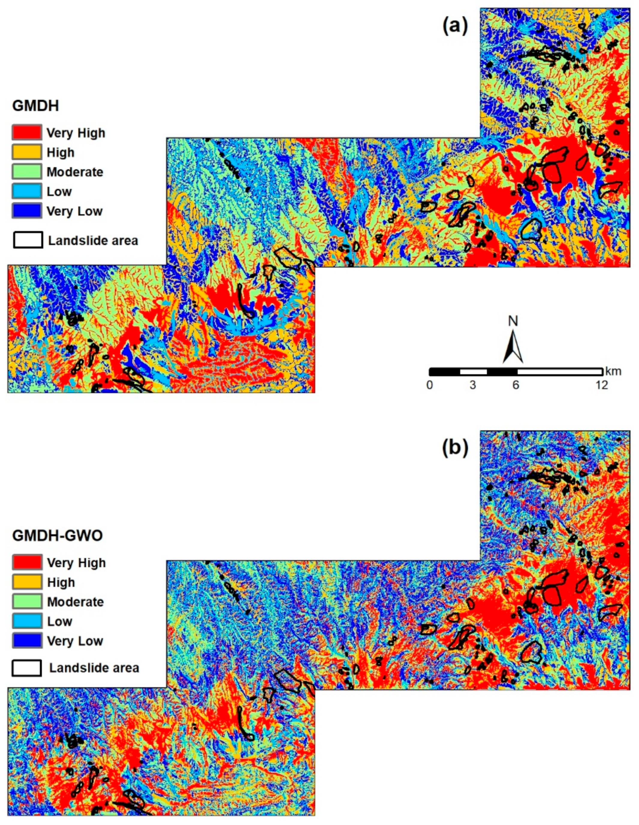
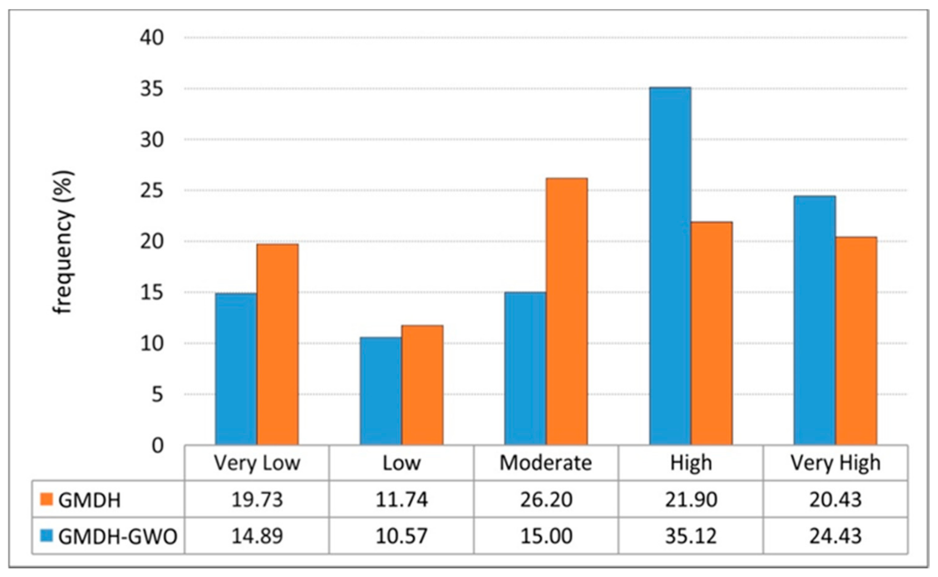
After training each model successfully, the algorithms were used to compute the landslide probability occurrence index (LPOI). First, the data for the entire study area were converted into raster format, with the same pixel size as the DEM. Next, the trained models were used to calculate the LPOI for each pixel of the study area. Then, the LPOI values were converted for compatibility with ArcGIS 10.2 to generate the landslide susceptibility maps. Finally, the LPOIs were divided into very low, low, moderate, high, and very high landslide susceptibility quantiles (Figure 5a,b). The use of quantiles is one of the most popular approaches for natural hazard probability classification. Ayalew et al. [64] and Akgun et al. [65] found that the quantile approach was superior when the LPOIs have positive or negative skewness.
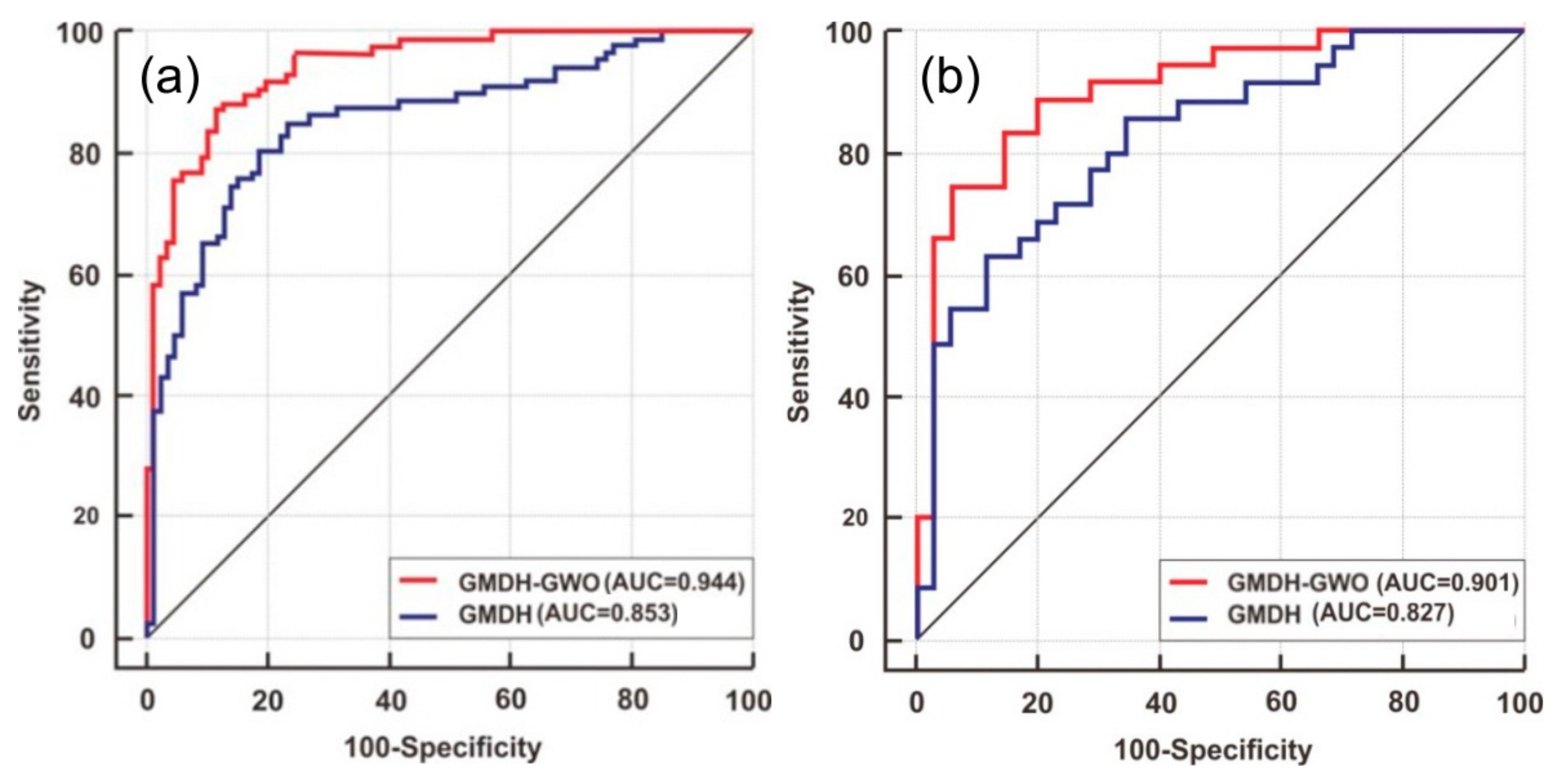
The landslide susceptibility maps attained in this study were validated using the testing dataset and ROC curve analysis. The findings showed that the GMDH model using the GWO (GMDH–GWO model) had better predictive power than the standard GMDH model in both the training and testing phases. The standard GMDH and GMDH–GWO models had AUC values of 0.853 and 0.944 for the training dataset and 0.827 and 0.901 for the testing dataset, respectively, equating to accuracies of 82% and 90%, respectively (Figure 6). The GMDH–GWO model was superior to the standard GMDH model in the training and testing phases, by 9.6% and 8.5%, respectively.
Moderate-susceptibility areas in the GMDH model were classified as highly landslide prone by the GMDH–GWO model. Thus, the standard GMDH model was less accurate in calculating the LPOI than the GMDH–GWO model. The standard GMDH and GMDH–GWO models considered most of the study area to be of moderate- and high susceptibility, respectively. As shown in Figure 7, the standard GMDH model predicted that approximately 19.73%, 11.74%, 26.20%, 21.90%, and 20.43% of the study area was very low, low, moderate, high, and very high landslide susceptibility area, whereas the respective values for the GMDH–GWO model were 14.89%, 10.57%, 15.00%, 35.12%, and 24.43%, respectively. The proportion of very high landslide susceptibility area was 4.00% lower according to the standard GMDH model relative to the GMDH–GWO model.

5. Discussion

The result indicates that probably of landslide occurrences increased up to a given altitude and then again reduced. This is due to the thinner soil at very high altitudes, and more rocks. Landslide probability was highest with southwest and south because of their higher soil moisture (in turn due to lower solar radiation) in these aspects compare with other ones. Landslide probability was also greater with longer LS. In fact, the longer LS, the more gravitational acceleration can affect detach part of the hillslope [47]. Distance from river more than 590 m has the lowest effect on the landslide occurrence in the study area and shows that river can be a potential source of the landslide occurrence. Regarding to the distance from the road, the more distance the lower landslide probability happens which shows that cutting the hillslopes make them prone to landslide occurrences. Regarding slope degree, for shallow slopes, the weak gravitational force is insufficient to cause downward movement of soil, while the soil on very steep slopes is relatively thin. Thus, only 6–13° (i.e., moderate) slopes in the study area promoted landslide occurrences. Finally, the landslide occurrence probability was higher when valley depth was lower. These findings are in accordance with previous results [4,5].
In addition, percentage of landslide locations within each class of landslide susceptibility map is shown in Figure 8. It shows that the most numbers of landslides fall into very high classes and this shows the high performance of the developed models. As shown in Figure 5, most of the study areas are prone to landslides. Through visual comparison of the landslide susceptibility and landslide conditioning factor maps, it was obvious that high/very high susceptibility to landslides was strongly associated with altitude, LS, valley depth, and slope degree.
According to the literature, the predictive power of a given model depends not only on the data quality, but also on the algorithms and assumptions used during model development [16]. More flexible models are better for modeling complex processes, such as natural hazards. Our GMDH–GWO model benefitted from both algorithms; inclusion of a second algorithm can overcome weaknesses in the base model. This is in accordance with [26], who also stated that ineffective conditioning factors reduce model performance. The high predictive power of the GMDH–GWO model in the current study (90%) indicated that all of the conditioning factors were effective in increasing model performance. The susceptibility map in this study could facilitate landslide hazard mitigation, by justifying prevention of any construction and urban development in high-susceptibility areas.

6. Conclusions

Although landslide risk reduction is important, landslide occurrence is a complicated process that cannot be predicted accurately using simple models; thus, in the present study, standard GMDH and GMDH–GWO models were applied to generate a landslide susceptibility map for a specific region in Uzbekistan. The main findings were as follows:
  • Landslides were most likely in the study area at altitudes of 1420–1736 m, and with southwest slope aspects, an LS of 3.12–18.94 m, a distance from the river of 65–318 m, a distance from the road of 0–1440 m, a 6–9.7° slope, a TWI of −24 to −145, and a valley depth of 77–144 m.
  • The GWO enhanced the predictive power of the standard GMDH model.
  • The performance of the GMDH–GWO model was superior to that of the standard GMDH model in the training and testing phases, by 9.6% and 8.5%, respectively.
  • The GMDH–GWO and standard GMDH models had 90% and 82% landslide prediction accuracy, respectively.
  • The GMDH–GWO model classified 14.89%, 10.57%, 15.00%, 35.12%, and 24.43% of the study area as having very low, low, moderate, high, and very high susceptibility to future landslides.

Author Contributions

Azam Kadirhodjaev; Writing—Original draft preparation, Fatemeh Rezaie; collected data, statistical analysis and writing methods, Saro Lee and Moung-Jin Lee; provided critical insights and contributed to the final version of the paper. All authors have read and agreed to the published version of the manuscript.

Funding

This research received no external funding.

Acknowledgments

This research was supported by the Basic Research Project of the Korea Institute of Geoscience and Mineral Resources (KIGAM) and Project of Environmental Business Big Data Platform and Center Construction funded by the Ministry of Science and ICT. This research was conducted at the Korea Environment Institute (KEI) with support from ‘Future Forecasting Government Management Support: A Study on the Modeling of Climate and Environment for the Transition to Data Science’ funded by the National Research Council for Economics, Humanities and Social Sciences.

Conflicts of Interest

The authors declare that they have no known competing financial interests or personal relationships that could have appeared to influence the work reported in this paper.

References

  1. Chakraborty, S.; Pradhan, R. Development of GIS based landslide information system for the region of East Sikkim. Int. J. Comput. Appl. 2012, 49, 5–9. [Google Scholar] [CrossRef]
  2. Aleotti, P.; Chowdhury, R. Landslide hazard assessment: Summary review and new perspectives. Bull. Eng. Geol. Environ. 1999, 58, 21–44. [Google Scholar] [CrossRef]
  3. Goetz, S.; Dubayah, R. Advances in remote sensing technology and implications for measuring and monitoring forest carbon stocks and change. Carbon Manag. 2011, 2, 231–244. [Google Scholar] [CrossRef]
  4. Nohani, E.; Moharrami, M.; Sharafi, S.; Khosravi, K.; Pradhan, B.; Pham, B.T.; Lee, S.; Melesse, A.M. Landslide susceptibility mapping using different GIS-based bivariate models. Water 2019, 11, 1402. [Google Scholar] [CrossRef] [Green Version]
  5. Bui, D.T.; Tuan, T.A.; Klempe, H.; Pradhan, B.; Revhaug, I. Spatial prediction models for shallow landslide hazards: A comparative assessment of the efficacy of support vector machines, artificial neural networks, kernel logistic regression, and logistic model tree. Landslides 2016, 13, 361–378. [Google Scholar] [CrossRef]
  6. Youssef, A.M.; Pradhan, B.; Pourghasemi, H.R.; Abdullahi, S. Landslide susceptibility assessment at Wadi Jawrah Basin, Jizan region, Saudi Arabia using two bivariate models in GIS. Geosci. J. 2015, 19, 449–469. [Google Scholar] [CrossRef]
  7. Althuwaynee, O.F.; Pradhan, B.; Park, H.-J.; Lee, J.H. A novel ensemble bivariate statistical evidential belief function with knowledge-based analytical hierarchy process and multivariate statistical logistic regression for landslide susceptibility mapping. Catena 2014, 114, 21–36. [Google Scholar] [CrossRef]
  8. Pourghasemi, H.R.; Mohammady, M.; Pradhan, B. Landslide susceptibility mapping using index of entropy and conditional probability models in GIS: Safarood Basin, Iran. Catena 2012, 97, 71–84. [Google Scholar] [CrossRef]
  9. Shirzadi, A.; Saro, L.; Joo, O.H.; Chapi, K. A GIS-based logistic regression model in rock-fall susceptibility mapping along a mountainous road: Salavat Abad case study, Kurdistan, Iran. Nat. Hazards 2012, 64, 1639–1656. [Google Scholar] [CrossRef] [Green Version]
  10. Pourghasemi, H.R.; Pradhan, B.; Gokceoglu, C. Application of fuzzy logic and analytical hierarchy process (AHP) to landslide susceptibility mapping at Haraz watershed, Iran. Nat. Hazards 2012, 63, 965–996. [Google Scholar] [CrossRef]
  11. Neaupane, K.M.; Piantanakulchai, M. Analytic network process model for landslide hazard zonation. Eng. Geol. 2006, 85, 281–294. [Google Scholar] [CrossRef]
  12. Opricovic, S.; Tzeng, G.-H. Compromise solution by MCDM methods: A comparative analysis of VIKOR and TOPSIS. Eur. J. Oper. Res. 2004, 156, 445–455. [Google Scholar] [CrossRef]
  13. Najafabadi, R.M.; Ramesht, M.H.; Ghazi, I.; Khajedin, S.J.; Seif, A.; Nohegar, A.; Mahdavi, A. Identification of natural hazards and classification of urban areas by TOPSIS model (case study: Bandar Abbas city, Iran). Geomat. Nat. Hazards Risk 2016, 7, 85–100. [Google Scholar] [CrossRef]
  14. Khosravi, K.; Sartaj, M.; Tsai, F.T.-C.; Singh, V.P.; Kazakis, N.; Melesse, A.M.; Prakash, I.; Bui, D.T.; Pham, B.T. A comparison study of DRASTIC methods with various objective methods for groundwater vulnerability assessment. Sci. Total Environ. 2018, 642, 1032–1049. [Google Scholar] [CrossRef]
  15. Khosravi, K.; Shahabi, H.; Pham, B.T.; Adamowski, J.; Shirzadi, A.; Pradhan, B.; Dou, J.; Ly, H.-B.; Gróf, G.; Ho, H.L. A comparative assessment of flood susceptibility modeling using Multi-Criteria Decision-Making Analysis and Machine Learning Methods. J. Hydrol. 2019, 573, 311–323. [Google Scholar] [CrossRef]
  16. Khosravi, K.; Cooper, J.R.; Daggupati, P.; Pham, B.T.; Bui, D.T. Bedload transport rate prediction: Application of novel hybrid data mining techniques. J. Hydrol. 2020, 585, 124774. [Google Scholar] [CrossRef]
  17. Ngo, P.T.T.; Panahi, M.; Khosravi, K.; Ghorbanzadeh, O.; Karimnejad, N.; Cerda, A.; Lee, S. Evaluation of deep learning algorithms for national scale landslide susceptibility mapping of Iran. Geosci. Front. 2020. [Google Scholar] [CrossRef]
  18. Lee, S. Landslide susceptibility mapping using an artificial neural network in the Gangneung area, Korea. Int. J. Remote Sens. 2007, 28, 4763–4783. [Google Scholar] [CrossRef]
  19. Pascale, S.; Parisi, S.; Mancini, A.; Schiattarella, M.; Conforti, M.; Sole, A.; Murgante, B.; Sdao, F. Landslide susceptibility mapping using artificial neural network in the urban area of Senise and San Costantino Albanese (Basilicata, Southern Italy). In Proceedings of the International Conference on Computational Science and Its Applications, Ho Chi Minh City, Vietnam, 24–27 June 2013; pp. 473–488. [Google Scholar]
  20. Shahri, A.A.; Spross, J.; Johansson, F.; Larsson, S. Landslide susceptibility hazard map in southwest Sweden using artificial neural network. Catena 2019, 183, 104225. [Google Scholar] [CrossRef]
  21. Choubin, B.; Darabi, H.; Rahmati, O.; Sajedi-Hosseini, F.; Kløve, B. River suspended sediment modelling using the CART model: A comparative study of machine learning techniques. Sci. Total Environ. 2018, 615, 272–281. [Google Scholar] [CrossRef]
  22. Lee, S.; Panahi, M.; Pourghasemi, H.R.; Shahabi, H.; Alizadeh, M.; Shirzadi, A.; Khosravi, K.; Melesse, A.M.; Yekrangnia, M.; Rezaie, F. Sevucas: A novel gis-based machine learning software for seismic vulnerability assessment. Appl. Sci. 2019, 9, 3495. [Google Scholar] [CrossRef] [Green Version]
  23. Panahi, M.; Gayen, A.; Pourghasemi, H.R.; Rezaie, F.; Lee, S. Spatial prediction of landslide susceptibility using hybrid support vector regression (SVR) and the adaptive neuro-fuzzy inference system (ANFIS) with various metaheuristic algorithms. Sci. Total Environ. 2020, 741, 139937. [Google Scholar] [CrossRef]
  24. Dehnavi, A.; Aghdam, I.N.; Pradhan, B.; Varzandeh, M.H.M. A new hybrid model using step-wise weight assessment ratio analysis (SWARA) technique and adaptive neuro-fuzzy inference system (ANFIS) for regional landslide hazard assessment in Iran. Catena 2015, 135, 122–148. [Google Scholar] [CrossRef]
  25. Polykretis, C.; Chalkias, C.; Ferentinou, M. Adaptive neuro-fuzzy inference system (ANFIS) modeling for landslide susceptibility assessment in a Mediterranean hilly area. Bull. Eng. Geol. Environ. 2019, 78, 1173–1187. [Google Scholar] [CrossRef]
  26. Bui, D.T.; Khosravi, K.; Tiefenbacher, J.; Nguyen, H.; Kazakis, N. Improving prediction of water quality indices using novel hybrid machine-learning algorithms. Sci. Total Environ. 2020, 721, 137612. [Google Scholar] [CrossRef] [PubMed]
  27. Ballabio, C.; Sterlacchini, S. Support vector machines for landslide susceptibility mapping: The Staffora River Basin case study, Italy. Math. Geosci. 2012, 44, 47–70. [Google Scholar] [CrossRef]
  28. Lee, S.; Hong, S.-M.; Jung, H.-S. A support vector machine for landslide susceptibility mapping in Gangwon Province, Korea. Sustainability 2017, 9, 48. [Google Scholar] [CrossRef] [Green Version]
  29. Dou, J.; Yunus, A.P.; Bui, D.T.; Merghadi, A.; Sahana, M.; Zhu, Z.; Chen, C.-W.; Khosravi, K.; Yang, Y.; Pham, B.T. Assessment of advanced random forest and decision tree algorithms for modeling rainfall-induced landslide susceptibility in the Izu-Oshima Volcanic Island, Japan. Sci. Total Environ. 2019, 662, 332–346. [Google Scholar] [CrossRef]
  30. Pham, B.T.; Khosravi, K.; Prakash, I. Application and comparison of decision tree-based machine learning methods in landside susceptibility assessment at Pauri Garhwal Area, Uttarakhand, India. Environ. Process. 2017, 4, 711–730. [Google Scholar] [CrossRef]
  31. Pham, B.T.; Prakash, I.; Khosravi, K.; Chapi, K.; Trinh, P.T.; Ngo, T.Q.; Hosseini, S.V.; Bui, D.T. A comparison of Support Vector Machines and Bayesian algorithms for landslide susceptibility modelling. Geocarto Int. 2019, 34, 1385–1407. [Google Scholar] [CrossRef]
  32. Hong, H.; Liu, J.; Bui, D.T.; Pradhan, B.; Acharya, T.D.; Pham, B.T.; Zhu, A.-X.; Chen, W.; Ahmad, B.B. Landslide susceptibility mapping using J48 Decision Tree with AdaBoost, Bagging and Rotation Forest ensembles in the Guangchang area (China). Catena 2018, 163, 399–413. [Google Scholar] [CrossRef]
  33. Tien Bui, D.; Shirzadi, A.; Shahabi, H.; Geertsema, M.; Omidvar, E.; Clague, J.J.; Thai Pham, B.; Dou, J.; Talebpour Asl, D.; Bin Ahmad, B. New ensemble models for shallow landslide susceptibility modeling in a semi-arid watershed. Forests 2019, 10, 743. [Google Scholar] [CrossRef] [Green Version]
  34. Di Napoli, M.; Carotenuto, F.; Cevasco, A.; Confuorto, P.; Di Martire, D.; Firpo, M.; Pepe, G.; Raso, E.; Calcaterra, D. Machine learning ensemble modelling as a tool to improve landslide susceptibility mapping reliability. Landslides 2020, 17, 1897–1914. [Google Scholar] [CrossRef]
  35. Khodadadi, F.; Entezari, M.; Sasanpour, F. Analysis of Geomorphologic Hazards of Landslide and Flood using VIKOR-AHP and Fr Models in the Alborz Province. Phys. Geogr. Res. Q. 2019, 51, 183–199. [Google Scholar] [CrossRef]
  36. Chen, W.; Hong, H.; Panahi, M.; Shahabi, H.; Wang, Y.; Shirzadi, A.; Pirasteh, S.; Alesheikh, A.A.; Khosravi, K.; Panahi, S. Spatial prediction of landslide susceptibility using gis-based data mining techniques of anfis with whale optimization algorithm (woa) and grey wolf optimizer (gwo). Appl. Sci. 2019, 9, 3755. [Google Scholar] [CrossRef] [Green Version]
  37. Ebtehaj, I.; Bonakdari, H. A support vector regression-firefly algorithm-based model for limiting velocity prediction in sewer pipes. Water Sci. Technol. 2016, 73, 2244–2250. [Google Scholar] [CrossRef] [Green Version]
  38. Shaghaghi, S.; Bonakdari, H.; Gholami, A.; Ebtehaj, I.; Zeinolabedini, M. Comparative analysis of GMDH neural network based on genetic algorithm and particle swarm optimization in stable channel design. Appl. Math. Comput. 2017, 313, 271–286. [Google Scholar] [CrossRef]
  39. Reichenbach, P.; Rossi, M.; Malamud, B.D.; Mihir, M.; Guzzetti, F. A review of statistically-based landslide susceptibility models. Earth-Sci. Rev. 2018, 180, 60–91. [Google Scholar] [CrossRef]
  40. Dodangeh, E.; Panahi, M.; Rezaie, F.; Lee, S.; Bui, D.T.; Lee, C.-W.; Pradhan, B. Novel hybrid intelligence models for flood-susceptibility prediction: Meta optimization of the GMDH and SVR models with the genetic algorithm and harmony search. J. Hydrol. 2020, 590, 125423. [Google Scholar] [CrossRef]
  41. Nguyen, V.V.; Pham, B.T.; Vu, B.T.; Prakash, I.; Jha, S.; Shahabi, H.; Shirzadi, A.; Ba, D.N.; Kumar, R.; Chatterjee, J.M. Hybrid machine learning approaches for landslide susceptibility modeling. Forests 2019, 10, 157. [Google Scholar] [CrossRef] [Green Version]
  42. Shirzadi, A.; Soliamani, K.; Habibnejhad, M.; Kavian, A.; Chapi, K.; Shahabi, H.; Chen, W.; Khosravi, K.; Thai Pham, B.; Pradhan, B. Novel GIS based machine learning algorithms for shallow landslide susceptibility mapping. Sensors 2018, 18, 3777. [Google Scholar] [CrossRef] [PubMed]
  43. Chen, W.; Chen, X.; Peng, J.; Panahi, M.; Lee, S. Landslide susceptibility modeling based on ANFIS with teaching-learning-based optimization and Satin bowerbird optimizer. Geosci. Front. 2020, 12, 93–107. [Google Scholar] [CrossRef]
  44. Thai Pham, B.; Prakash, I.; Dou, J.; Singh, S.; Trinh, P.; Trung Tran, H.; Minh Le, T.; Tran, V.; Kim Khoi, D.; Shirzadi, A. A novel hybrid approach of landslide susceptibility modeling using rotation forest ensemble and different base classifiers. Geocarto Int. 2018, 14, 1–38. [Google Scholar] [CrossRef]
  45. Feuillet, T.; Coquin, J.; Mercier, D.; Cossart, E.; Decaulne, A.; Jónsson, H.P.; Sæmundsson, Þ. Focusing on the spatial non-stationarity of landslide predisposing factors in northern Iceland: Do paraglacial factors vary over space? Prog. Phys. Geogr. 2014, 38, 354–377. [Google Scholar] [CrossRef]
  46. Menking, J.A.; Han, J.; Gasparini, N.M.; Johnson, J.P. The effects of precipitation gradients on river profile evolution on the Big Island of Hawai’i. GSA Bull. 2013, 125, 594–608. [Google Scholar] [CrossRef] [Green Version]
  47. Hong, H.; Naghibi, S.A.; Pourghasemi, H.R.; Pradhan, B. GIS-based landslide spatial modeling in Ganzhou City, China. Arab. J. Geosci. 2016, 9, 112. [Google Scholar] [CrossRef]
  48. Ivakhnenko, A.G. The group method of data of handling; a rival of the method of stochastic approximation. Sov. Autom. Control 1968, 13, 43–55. [Google Scholar]
  49. Jiang, Y.; Liu, S.; Peng, L.; Zhao, N. A novel wind speed prediction method based on robust local mean decomposition, group method of data handling and conditional kernel density estimation. Energy Convers. Manag. 2019, 200, 112099. [Google Scholar] [CrossRef]
  50. Mohebbian, M.R.; Dinh, A.; Wahid, K.; Alam, M.S. Blind, Cuff-less, Calibration-Free and Continuous Blood Pressure Estimation using Optimized Inductive Group Method of Data Handling. Biomed. Signal Process. Control 2020, 57, 101682. [Google Scholar] [CrossRef]
  51. Zhu, W.; Wang, J.; Zhang, W.; Sun, D. Short-term effects of air pollution on lower respiratory diseases and forecasting by the group method of data handling. Atmos. Environ. 2012, 51, 29–38. [Google Scholar] [CrossRef]
  52. Rostami, A.; Hemmati-Sarapardeh, A.; Karkevandi-Talkhooncheh, A.; Husein, M.M.; Shamshirband, S.; Rabczuk, T. Modeling heat capacity of ionic liquids using group method of data handling: A hybrid and structure-based approach. Int. J. Heat Mass Transf. 2019, 129, 7–17. [Google Scholar] [CrossRef]
  53. Stefenon, S.F.; Ribeiro, M.H.D.M.; Nied, A.; Mariani, V.C.; dos Santos Coelho, L.; da Rocha, D.F.M.; Grebogi, R.B.; de Barros Ruano, A.E. Wavelet group method of data handling for fault prediction in electrical power insulators. Int. J. Electr. Power Energy Syst. 2020, 123, 106269. [Google Scholar] [CrossRef]
  54. Najafzadeh, M.; Barani, G.-A.; Hessami-Kermani, M.-R. Group method of data handling to predict scour depth around vertical piles under regular waves. Sci. Iran. 2013, 20, 406–413. [Google Scholar] [CrossRef]
  55. Mirjalili, S.; Mirjalili, S.M.; Lewis, A. Grey wolf optimizer. Adv. Eng. Softw. 2014, 69, 46–61. [Google Scholar] [CrossRef] [Green Version]
  56. Gupta, S.; Deep, K. An opposition-based chaotic grey wolf optimizer for global optimisation tasks. J. Exp. Theor. Artif. Intell. 2019, 31, 751–779. [Google Scholar] [CrossRef]
  57. Tu, Q.; Chen, X.; Liu, X. Hierarchy strengthened grey wolf optimizer for numerical optimization and feature selection. IEEE Access 2019, 7, 78012–78028. [Google Scholar] [CrossRef]
  58. Niu, M.; Wang, Y.; Sun, S.; Li, Y. A novel hybrid decomposition-and-ensemble model based on CEEMD and GWO for short-term PM2. 5 concentration forecasting. Atmos. Environ. 2016, 134, 168–180. [Google Scholar] [CrossRef]
  59. Long, W.; Jiao, J.; Liang, X.; Tang, M. An exploration-enhanced grey wolf optimizer to solve high-dimensional numerical optimization. Eng. Appl. Artif. Intell. 2018, 68, 63–80. [Google Scholar] [CrossRef]
  60. Kaveh, A.; Zakian, P. Improved GWO algorithm for optimal design of truss structures. Eng. Comput. 2018, 34, 685–707. [Google Scholar] [CrossRef]
  61. Luo, K.; Zhao, Q. A binary grey wolf optimizer for the multidimensional knapsack problem. Appl. Soft Comput. 2019, 83, 105645. [Google Scholar] [CrossRef]
  62. Chung, C.-J.F.; Fabbri, A.G. Validation of spatial prediction models for landslide hazard mapping. Nat. Hazards 2003, 30, 451–472. [Google Scholar] [CrossRef]
  63. Jaafari, A.; Zenner, E.K.; Pham, B.T. Wildfire spatial pattern analysis in the Zagros Mountains, Iran: A comparative study of decision tree based classifiers. Ecol. Inform. 2018, 43, 200–211. [Google Scholar] [CrossRef]
  64. Ayalew, L.; Yamagishi, H. The application of GIS-based logistic regression for landslide susceptibility mapping in the Kakuda-Yahiko Mountains, Central Japan. Geomorphology 2005, 65, 15–31. [Google Scholar] [CrossRef]
  65. Akgun, A.; Kıncal, C.; Pradhan, B. Application of remote sensing data and GIS for landslide risk assessment as an environmental threat to Izmir city (west Turkey). Environ. Monit. Assess. 2012, 184, 5453–5470. [Google Scholar] [CrossRef]
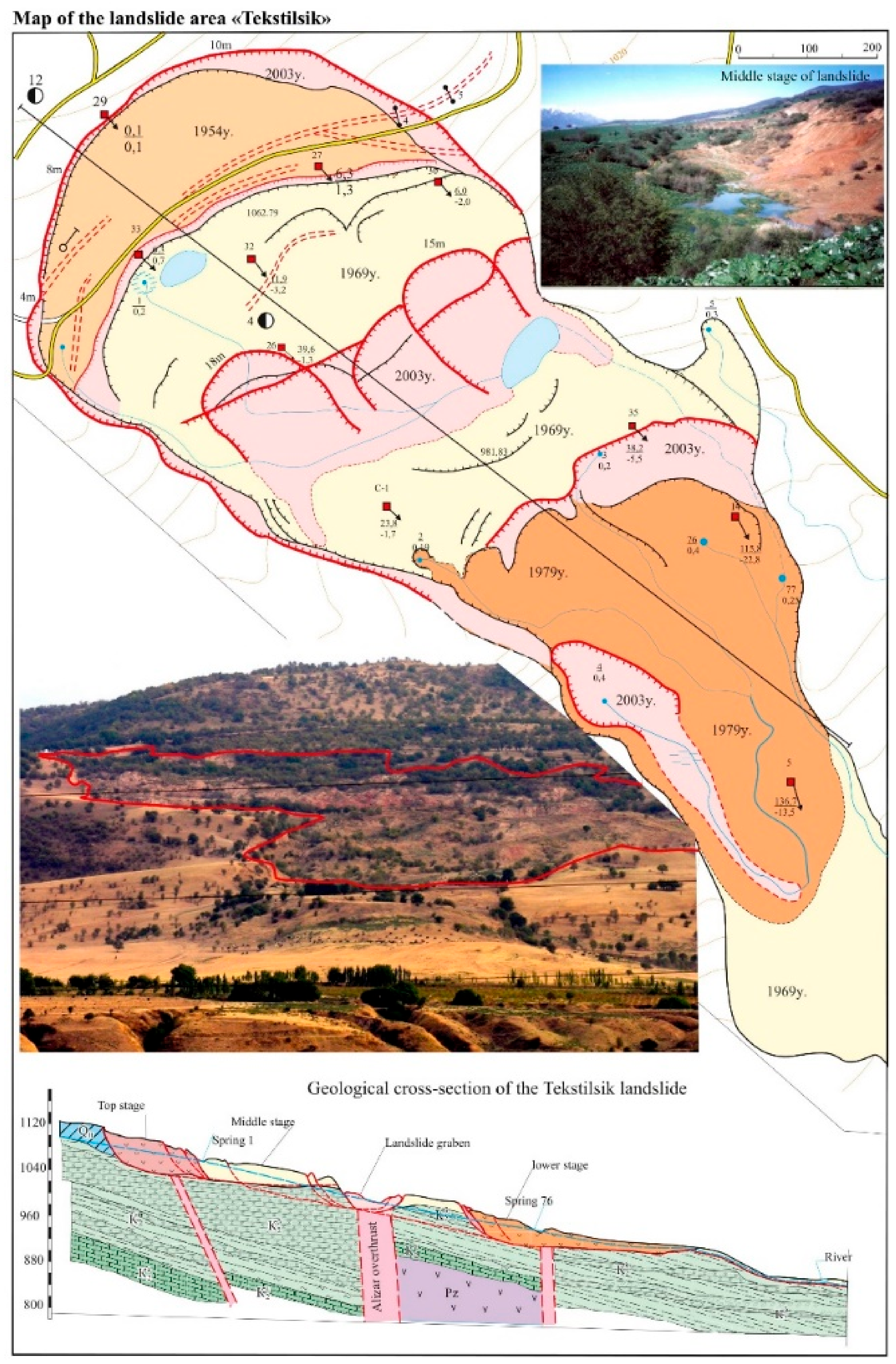
Figure 1. Map and cross-section of the Tekstilsik landslide.
Ijgi 09 00566 g001
Figure 2. Location of study area (left) and historical landslide locations (right).
Ijgi 09 00566 g002
Figure 3. Landslide conditioning factors in the study area: (a) Altitude; (b) Slope; (c) Aspect; (d) Valley Depth; (e) TWI; (f) LS; (g) Distance from Roads; (h) Distance from Rivers; (i) Geology.
Ijgi 09 00566 g003
Figure 4. The procedures overview to prepare the landslide susceptibility maps.
Ijgi 09 00566 g004
Figure 5. Landslide susceptibility map obtained using (a) standard group method of data handling (GMDH); (b) GMDH–gray wolf optimizer (GWO) models.
Ijgi 09 00566 g005
Figure 6. Model performance evaluation: (a) Training phase; (b) Testing phase.
Ijgi 09 00566 g006
Figure 7. Landslide area percentage in different susceptibility zones.
Ijgi 09 00566 g007
Figure 8. Percentage of landslide events within each class of landslide susceptibility map.
Ijgi 09 00566 g008
Table 1. Summarize of the literature review.
AuthorsModels
Nohani et al. [4]FR
Youssef et al. [6]WOE
Althuwaynee [7] EBF
Pourghasemi et al. [8]SE
Shirzadi et al. [9]LR
Pourghasemi et al. [10]AHP
Neaupane et al. [11]ANP
Khodadadi et al. [35]VIKOR
Najafabadi et al. [13]TOPSIS
Lee et al. [18]; Pascale et al. [19] and Shahri et al. [20]ANN
Panahi et al. [23]; Dehnavi et al. [24] and Polykretis et al. [25]ANFIS
Dou et al. [29]RF
Chen at al. (2018) [36]kernel logistic regression
Pham et al. [30]RF, LMT, BFDT, CART
Pham et al. [31]NBT, BN and NB
Honge et al. [32]AdaBoost, Bagging and RF
Bui et al. [33]SVM
Napoli et al. [34]ANN and
Ngo et al. [17]Deep learning (RNN and CNN)
Table 2. Hazardous geological processes (HGP) documented in the Tekstilsik area.
NoYear of HGPType of HGPCharacteristics of HGP
11966Suffusion (subsoil erosion)-
21969CrackL = up to 500 m
31973Activation of cracksL = up to 550 m
41979Landslide22.5 million m3
51981CrackL = up to 70 m
61987Landslide6.8 thousand m3
71994Landslide3.0 million m3
82003Landslide1.5 million m3
92004CrackL = up to 20 m
102005CrackL = up to 450 m
112016CrackL = 7 m
122017CrackL = up to 60 m
Table 3. Impact of conditioning factor subclasses on landslide probability using FR model.
Conditioning FactorsClassesNumber of PixelsNumber of LandslideFR
Altitude (m)837–1137155,8547640.20
1137–1275155,70825210.66
1275–1420155,50350561.32
1420–1736155,24174831.96
1736–3201155,06832860.86
Slope (degree)0–6.09150,70936930.99
6.09–9.74152,90749961.32
9.74–13.64155,56341631.08
13.64–19.25160,61737470.94
19.25–62.13152,24125110.67
AspectFlat45671070.95
North133,38233581.02
Northeast128,34431020.98
East59,41015981.09
Southeast42,6047520.71
South58,57418671.29
Southwest95,19831831.35
West117,35226190.90
Northwest132,60625250.77
Valley depth77.87–144.92154,15423471.54
144.92–203.02155,48259011.36
203.02–258.88157,52952710.97
258.88–502.47150,11935810.51
TWI−2.59–−0.59140,90623350.67
−59–−0.71161,56928450.72
−0.71–−1.18164,11736640.91
−1.18–−24.98161,01148451.22
−24.98–−145.25149,77154221.47
−145.25<140,90623350.62
LS0–2.00108,56417300.65
2.00–2.30185,62935000.77
2.30–2.60167,55537420.91
2.60–3.12162,27146271.16
3.12–18.94153,35555121.46
Distance from Roads (m)0–617.19160,97251551.35
617.19–1440.12160,51452071.36
1440.12–2365.92160,47650541.32
2365.92–3566.02160,43029180.76
3566.02–8743.62160,3707770.20
Distance from Rivers (m)0–65.90164,91641861.07
65.90–164.75160,62842121.10
164.75–318.52162,06942471.10
318.52–593.11158,50139961.06
593.11–2800.80156,53424710.66
GeologyC1-215,3301960.61
J91,031530.03
K60,7245840.46
N415,32571230.82
P34,98413401.84
P121,524460.10
QIaz21,7841490.33
QIIkr96,83327691.37
QIIIsk115,30762892.62
QIVam23,8325601.13
other21,60600.00