Article

Three-Dimensional (3D) Parametric Modeling and Organization for Web-Based Visualization of City-Scale Pipe Network

1
GNSS Research Center, Wuhan University, Wuhan 430072, China
2
School of Transportation, Wuhan University of Technology, Wuhan 430063, China
*
Author to whom correspondence should be addressed.
ISPRS Int. J. Geo-Inf. 2020, 9(11), 623; https://doi.org/10.3390/ijgi9110623
Submission received: 11 September 2020 / Revised: 22 October 2020 / Accepted: 23 October 2020 / Published: 24 October 2020

Abstract

:
Underground pipe network is a critical city infrastructure, which plays an important role in smart city management. As the detailed three-dimensional (3D) scene of underground pipe networks is difficult to construct, and massive numbers of pipe points and segments are difficult to manage, a 3D pipe network modeling and organization method is explored in this study. First, the modeling parameters were parsed from the pipe network survey data. Then, the 3D pipe segment and point models were built based on parametric modeling algorithms. Finally, a heterogeneous data structure for the 3D pipe network was established through loose quadtree data organization. The proposed data structure was suitable for 3D Tiles, which was adopted by Cesium (a web-based 3D virtual globe); hence, a multitude of pipe networks can be viewed in the browser. The proposed method was validated by generating and organizing a large-scale 3D pipe network scene of Beijing. The experimental results indicate that the 3D pipe network models formed by this method can satisfy the visual effect and render the efficiency required for smart urban management.

1. Introduction

Urban underground pipe networks are essential infrastructure and are used to supply gas, water, electricity, communications, drainage, etc. [1]. With the rapid development of cities, many types of underground pipelines have been constructed, making underground spaces more complex. Effective underground space management is considered a ‘Gordian knot’ [2]. In recent years, China has launched a national program with aims to effectively manage underground pipe networks based on comprehensive pipe network surveying data and geoinformation systems [3].
The visualization of the urban underground pipe network has been studied by many researchers, with a focus on automatic pipeline modeling and three-dimensional (3D) visualization [4,5,6]. Early technologies used in geographic information systems (GIS) and computer-aided design (CAD) software for pipeline visualization were based on two-dimensional (2D) maps consisting of points and lines [7,8]. Although the direction of the pipelines can be roughly presented, the spatial relationship of the pipelines cannot be directly described. With the development of 3D visualization technology, the visualization of underground objects in 3D form has attracted much more attention [9]. In order to avoid the gap between 3D pipeline segments, Du and Zlatanova [10] presented an approach by constructing a new pipe to connect the pipes for visualization. However, the semantic characteristics of the pipe points were not studied. Becker et al. [11] proposed a new spatial information model that considered the semantic characteristics of pipe points. This model has already been integrated into City Geography Markup Language (CityGML) [12], but the visualization of city-scale underground facility networks was not explored. Wu et al. [13] realized the 3D visualization of city-scale pipelines using the graphics processing unit (GPU)-based ray casting method, which divides data into blocks and uses a geometry shader for each pipeline. However, this approach is not flexible and does not consider the matching between the pipe segments of different diameters and pipe point models. In addition, the method was implemented based on the client program, which cannot be accessed through a browser. Although these studies above presented promising results, they do not meet the requirements of underground space planning [14]. With the development of cloud computing and web service, transforming the platform into a web browser is important for sharing and cooperation. The visualization of underground pipe networks for urban management should meet: (1) large-scale continuous visualizations in the web environment; (2) accurate descriptions of the semantic characteristics of pipe points. Accurately modeling the characteristics of the pipe point model and adopting them to the city-scale visualization of pipe networks are essential. Therefore, accurately and quickly establishing a 3D pipeline model based on raw 2D pipeline data and accurately visualizing the semantics of pipe points in a 3D web scene are vital for urban underground pipeline management [15].
Improvements in computer hardware performance and browser technology, especially WebGL development, have greatly promoted web 3D visualization [16]. Cesium [17], a cross-platform virtual earth platform based on JavaScript, has gradually been recognized by Open Geospatial Consortium (OGC). In particular, the open-source standard 3D Tiles [18] introduced in 2015 can provide streaming processes for many heterogeneous 3D geographical targets, allowing the visualization of all geographical data types possibility. The 3D Tiles specification [19] has been highly recommended by the Cesium developer community. 3D Tiles support the streaming of data such as vector, raster, model, and point cloud. Inspired by research on processing building information modeling (BIM) data into 3D Tiles [20], we selected the 3D Tiles format for pipeline visualization in the web environment. This kind of pipeline visualization has already been investigated by other researchers. Jurado et al. [21] proposed a Web-based GIS application to study the real-time visualization of underground infrastructure. Wang et al. [22] proposed a hybrid framework for the high-performance modeling of 3D pipe networks, which adopt 3D platform SuperMap and a spatial 3D model format. However, the visualization effect and efficiency of urban underground pipelines in a web environment still requires further investigation, in particular for keeping the additional semantic features through parametric modeling.
In this study, a parametric modeling approach for the 3D visualization of urban underground pipelines is proposed, and an optimized data organization suitable for 3D Tiles was presented based on Cesium. The remainder of this paper is organized as follows. The semantically parameterized 3D modeling for pipeline data and processing in Batched 3D Model (B3DM) for 3D Tiles specification is presented in Section 2. The verification and analysis of the experiment are described in Section 3, and the study is summarized and discussed in Section 4.

2. Pipeline Modeling and Organization

2.1. Workflow

The proposed method includes three key steps: (1) parsing geometric and semantic pipeline data from the database; (2) generating 3D models for pipe segments and points; (3) splitting and transforming 3D pipe models into B3DM data organized with 3D Tiles structure. The processing workflow is presented in Figure 1. In the first step, the parametric information is parsed from raw pipeline data in geographic database such as Microsoft Database (MDB). The second step consists of two parts: pipe segment modeling and pipe point modeling. Pipe segment modeling mainly includes mesh construction and texture mapping. Pipe point modeling requires the processing of special points, such as points at the connection of multiple pipe sections as well as points with special features. For better rendering efficiency, we introduced a variant of the quadtree to build the spatial index of models.

2.2. Pipe Network Data Structure

Pipe network data can be clarified into three types: pipe point, pipeline segment, and ancillary facility. The data structure of the pipe points as well as the pipeline segments are listed in Table 1 and Table 2, respectively. These tables provide the relevant fields for pipeline modeling with the method presented in Section 2.3 and Section 2.4.
The first step in pipeline modeling is to parse the properties of pipe point and pipe segment for modeling. MDB is a relational database storing data according to pipeline types. By parsing the layer data, the important characteristics of the pipe points for modeling, including coordinates, feature points, appendages, and so on, can be obtained. The information required for pipe segment modeling includes the starting and ending point IDs, depths, pipe diameters, and other key fields.

2.3. Parametric Modeling of Pipe Segment

To automatically model the pipe segments, a parametric modeling algorithm for the construction of the pipeline model based on survey data, e.g., pipe diameter and buried depth, is proposed. The automatic modeling of the pipeline mesh is the key purpose of the algorithm. Based on the data structure of the pipe segment, it is clear that each pipe segment is composed of two pipe points. According to the Chinese national pipeline standard [23], the length of each segment is typically no more than 70 m. The pipe point information contains 3D coordinates and attribute data. The spatial position of the pipe segment is determined by the coordinates of the start and end points as well as the buried depth. Furthermore, the diameter of the segment is used to describe the shape of the pipe surface as a square or circle. For example, 300 × 200 means that the pipe exhibits a square cross surface with 300 and 200 mm in width and length, respectively, whereas DN300 indicates that the cross surface is a circle with a diameter of 300 mm. Figure 2 illustrates the different types of pipe segment.

2.3.1. Pipe Segment Mesh Construction

For pipe segment modeling, the following steps are performed:
(1)
Obtaining the coordinates of the start and end points as well as the diameter of the pipe segment;
(2)
Calculating the coordinates of each vertex in the spatial coordinate system: three vertices are used to form a triangle, and all the triangles are spliced together to form the geometry of the pipe segment.
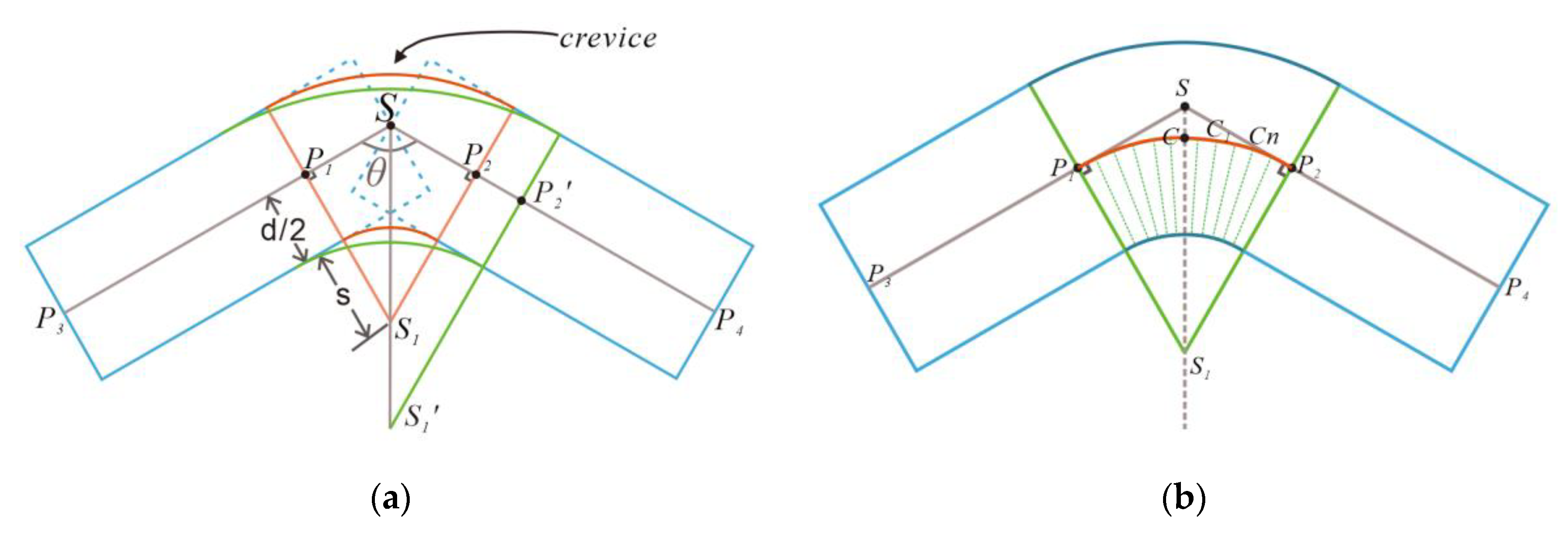
When the cylinder is converted into a polygonal column, the “segment number” parameter, controlling the smoothness of the pipeline, is required to subdivide the cylinder. The modeling of the curve part of the pipe segment is displayed in Figure 3.
As there are crevices between sections in the modeling method presented above, additional treatment is needed for crevice repairing. In order to solve the crevice problem, a smooth arc pipe segment is constructed. Figure 3a demonstrates the construction of suture for the crevice. Point S is the intersection point of the center line of the two-pipe segment, point P3 is the starting point of one pipe segment, and point P4 is the ending point of the other pipe segment. θ is the angle formed by the pipe segments SP3 as well as SP4. To determine the smooth arc segment, the center point S1 should be given first, and the 3D coordinates of S1 can be calculated as follows:
{ x s 1   =   x s + ( x p 1 + x p 2 2 x s ) × | S P 2 | | S P 1 + S P 2 | × cos 1 ( θ / 2 ) y s 1   =   y s + ( y p 1 + y p 2 2 y s ) × | S P 2 | | S P 1 + S P 2 | × cos 1 ( θ / 2 ) z s 1   =   z s + ( z p 1 + z p 2 2 z s ) × | S P 2 | | S P 1 + S P 2 | × cos 1 ( θ / 2 )
where | S P 2 | is the length of line segment SP2, | S P 1 + S P 2 | is the length of the addition vector of SP1 and SP2. P1 ( x p 1 , y p 1 , z p 1 ) and P2 ( x p 2 , y p 2 , z p 2 ) are the perpendicular intersection points of point S1 to SP3 and SP4. Their coordinates can be calculated as follows:
{ x p 1   =   x s + ( x p 3 x s ) × | S P 1 | | S P 3 | y p 1   =   y s + ( y p 3 y s ) × | S P 1 | | S P 3 | z p 1   =   z s + ( z p 3 z s ) × | S P 1 | | S P 3 |
{ x p 2   =   x s + ( x p 4 x s ) × | S P 2 | | S P 4 | y p 2   =   y s + ( y p 4 y s ) × | S P 2 | | S P 4 | z p 2   =   z s + ( z p 4 z s ) × | S P 2 | | S P 4 |
where | S P 3 | is the length of the line SP3, | S P 4 | is the length of line SP4. P3 ( x p 3 , y p 3 , z p 3 ) and P4 ( x p 4 , y p 4 , z p 4 ) are the endpoints of the pipe segment, and point S ( x s , y s , z s ) is the connection point of the two pipe segments. Their coordinates can be obtained from the raw pipeline data. Similarly, | S P 1 | is the distance from point S to point P1, | S P 2 | is the distance from point S to point P2. The length (L) of | S P 1 | can be calculated as follows:
L   =   | S P 1 |   =   | S P 2 |   =   | S 1 P 2 | tan ( θ / 2 )   =   ( d 2 + s ) / tan ( θ / 2 )
where segment, the center point S1 d is the diameter of the pipe segment, s is the vertical distance from the center point S 1 of the torus to the pipe, and it is a variable that controls the radius of the suture. In Figure 3a, the suture is an orange diagram when s equals the pipe radius, and green when s equals the pipe diameter. For a better crevice-repairing effect, the value of s is typically slightly larger than the pipe radius. In order to link P1 and P2, an arc is drawn with point S 1 as the center and | S 1 P 1 | as the radius. Point C is the intersection point of line   S S 1 and the arc. As the length of | C S 1 | equals   | S 1 P 1 | , thus, the coordinates of point C can be calculated as follows:
{ x c   =   x s 1 + ( x s x s 1 ) × | C S 1 | | S S 1 | y c   =   y s 1 + ( y s y s 1 ) × | C S 1 | | S S 1 | z c   =   z s 1 + ( z s z s 1 ) × | C S 1 | | S S 1 |
Point C n is in the plane formed by line S S 1 ,   S 1   P 2 , and C n are on the circumference of the circle with point S 1 as the center. Therefore, we can obtain the coordinates of C n ( x n , y n , z n ) with the formula below:
{ | S 1 P 2 |   =   ( x n x s 1 ) 2 + ( y n y s 1 ) 2 + ( z n z s 1 ) 2 0 = a ( x n x s 1 ) + b ( y n y s 1 ) + c ( z n z s 1 ) + t cos ( n β ) = ( x n x s 1 ) ( x p 2 x s 1 ) + ( y n y s 1 ) ( y p 2 y s 1 ) + ( z n z s 1 ) ( z p 2 z s 1 ) | S 1 P 1 | | S 1 P 2 |
where the lengths of | S 1 P 1 | and | S 1 P 2 | equal the radius of the suture arc, β is a user-defined minimum radian parameter that determines the smoothness of the suture grid, and a, b, c, and t can be obtained as the follows:
{ a   =   ( y s y s 1 ) ( z p 2 z s 1 ) ( y p 2 y s 1 ) ( z s z s 1 ) b   =   ( z s z s 1 ) ( x p 2 x s 1 ) ( z p 2 z s 1 ) ( x s x s 1 ) c   =   ( x s x s 1 ) ( y p 2 y s 1 ) ( x p 2 x s 1 ) ( y s y s 1 )
t   =   a x s 1 b y s 1 c z s 1
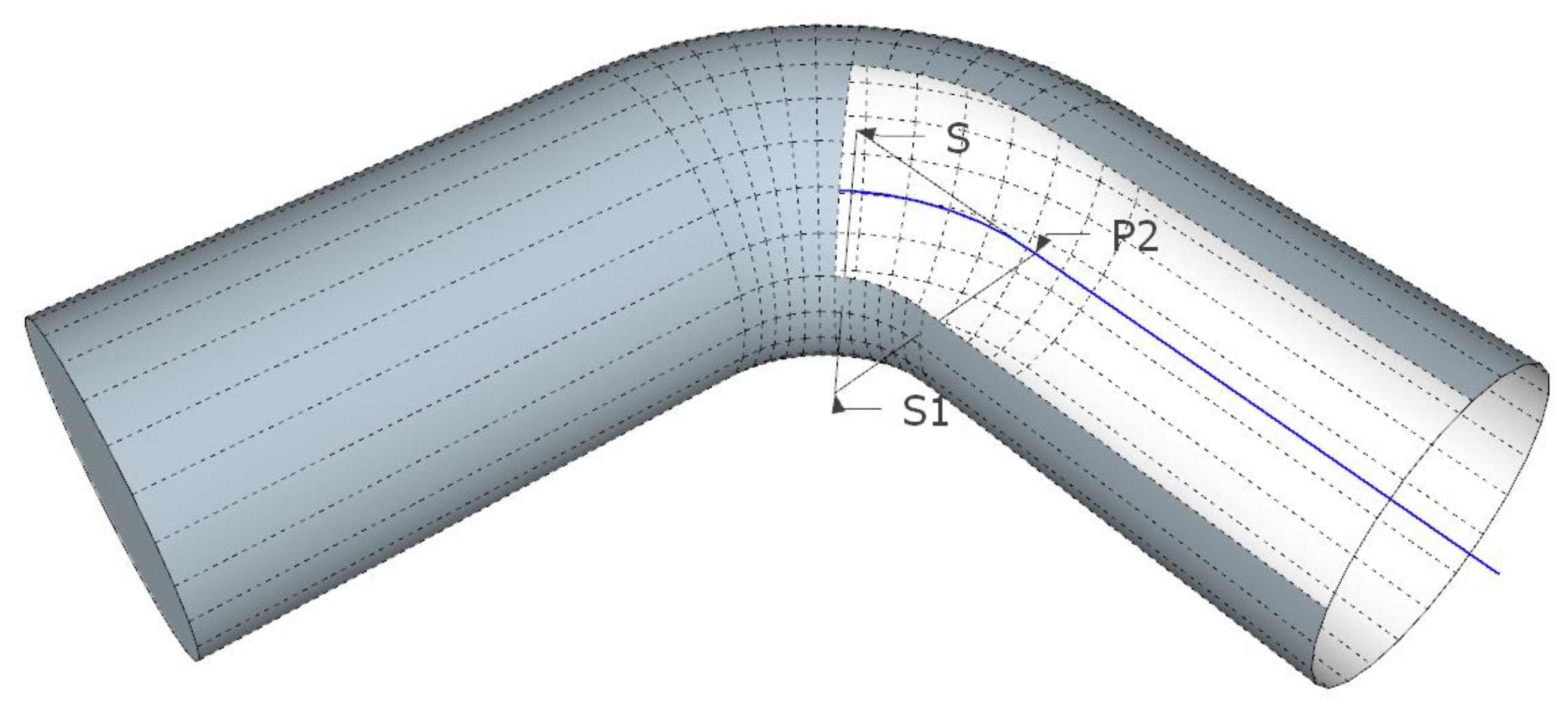
Therefore, using this series of centers ( C 1 , C 2 C n ) , the model of the pipeline suture can be constructed, as displays in Figure 4.
In general, the pipe segment model is determined by the start and end points as well as the properties of the pipe segment. The start and end points are 3D coordinates, and the pipe segment model coordinates are global, allowing the model to be placed in the correct position on the virtual earth.

2.3.2. Dynamic Texture Mapping

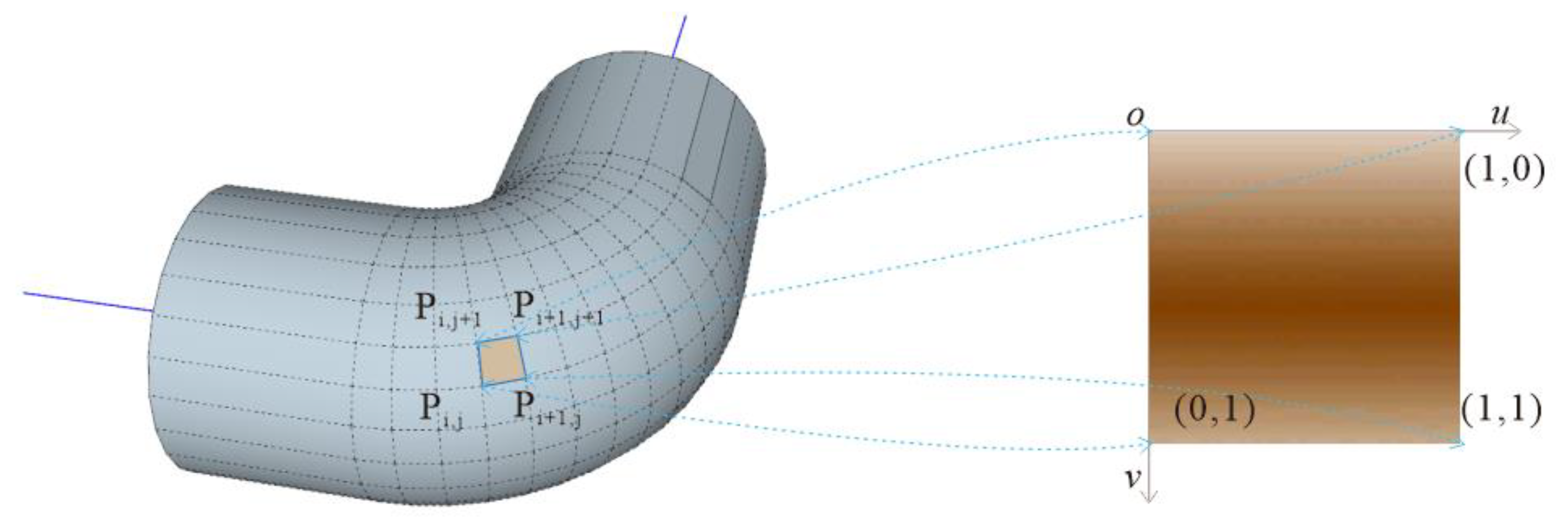
Texture mapping is a method that maps pixels from a texture to a 3D surface, and it can be interpreted as wrapping the image around the object. A dynamic texture has a spatially repetitive pattern with a time-varying visual pattern. For a better effect of the pipeline, a dynamic texture was used for texture mapping based on the pipeline mesh (Figure 5). In this subsection, the texture mapping method is presented. Dynamic texture mapping of the pipeline consists of two parts, one is the texture coordinate calculation, and the other is dynamic texture mapping [24].
(1) Texture coordinate calculation of the suture of the pipeline. Texture mapping at the pipe segment extends along the pipeline and vertical directions; however, texture mapping at the pipeline connection is more complex. According to the coordinates of the center point of the suture calculated with Equation (1), the spatial coordinates of the four corners can be obtained. The texture coordinates of the vertex P(i,j) on the mesh of suture can be calculated as follows:
{ U ( i , j )   =   | P ( i , j ) P ( i + 1 , j ) | n i V ( i , j )   =   V ( i 1 , j ) + | P ( i , j ) P ( i , j + 1 ) | n
where n is the basic tile length between the two sampling points, | P ( i , j ) P ( i + 1 , j ) | is the length of points P ( i , j ) and P ( i + 1 , j ) , and | P ( i , j ) P ( i , j + 1 ) | is the length of the points P ( i , j ) and P ( i , j + 1 ) . Here, (u,v) represents the texture coordinate system, where the u axis is along the pipeline direction, and the v axis coincides with the vertical direction. The range of texture coordinates is between (0,0) and (1,1). If it exceeds the range, the texture image will be mapped by GL_REPEAT approach of OpenGL.
(2) Dynamic texture mapping. To demonstrate the dynamic visualization effect in the system, the pipes for drainage and water supply are selected for the dynamic texture mapping. A dynamic Graphics Interchange Format figure was prepared in advance through an image stream to store the image sequences. The texture coordinate stays the same and refreshes the image for each frame in the rendering process, achieving a dynamic effect without re-computing the texture coordinates.

2.4. Parametric Modeling of Pipe-Point

Parametric modeling of a pipe-point is an algorithm for building a complex 3D pipe-point model based on the parameters such as pipe-point position, pipe segment direction, and pipe diameter. In the pipe-point parametric modeling algorithm, the fusion of the pipe-point prototype model and the pipe segment model is considered. The pipe-point prototype model refers to the 3D model built in advance with 3ds Max or other modeling software. Different types of models, such as water valve and flange, are prepared in the model library. In the process of the pipe point, the position translation, scaling, and rotation parameters of the pipe-point prototype model are calculated from adjacent pipeline data. The pipe point is simultaneously processed with the pipeline. Pipe-point modeling requires distinguishing between feature points and connection points. Feature points typically include water meters, valves, and inspection wells, while connection points refer to the elbow, tee, and cross. According to the diameter of each pipe and angle between pipe segments, the prototype model in the model library is automatically adjusted using the construction algorithm in order to much more effectively fuse the prototype model and pipe segment models.

2.4.1. Feature Point Processing

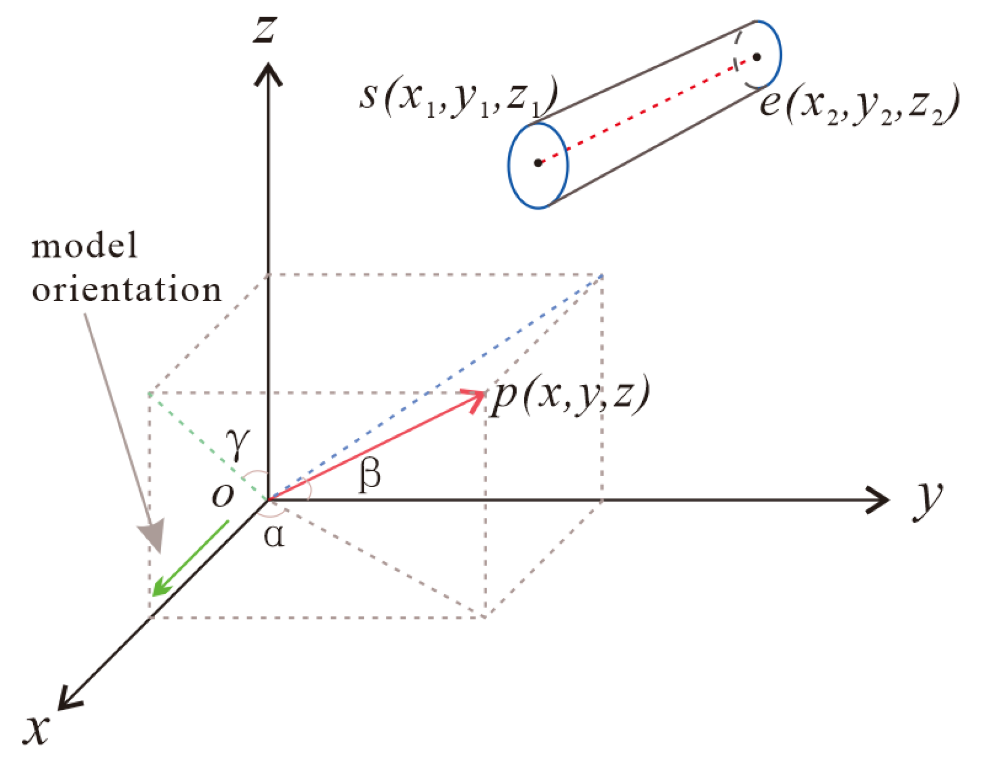
To improve the pipe network visualization accuracy, the prototype model library is prepared for feature points such as water meters, valves, and other pipe points. However, the orientation and diameter of each feature point in the real pipe network system are different; thus, seamlessly joining the prototype and pipe segment models according to the parameters is usually a difficulty in the modeling process. In Figure 6, the green arrow represents the initial orientation of the prototype model. In the pipe point modeling process, the rotation angle can be calculated using the relative relationship between the coordinates of the start and end point of the pipe, and the scaling factor can be obtained according to the proportion of the pipe diameter with respect to the size of the prototype model. The rotation angle is calculated as follows, where α, β, and γ represent the angles between the pipe segment and the x axis, y axis, as well as z axis, respectively:
{ α   =   tan 1 y 2 y 1 x 2 x 1 β   =   tan 1 z 2 z 1 y 2 y 1 γ   =   tan 1 x 2 x 1 z 2 z 1

2.4.2. Connection Point Processing

Adjacent pipes are typically connected by an elbow, and the connection requires special modeling. In 3D visualization, spatial transformation is required for a 3D model to be placed in an appropriate position (Figure 7). The model matrix is applied to transform the vertices from local coordinates to world coordinates. For a flange 3D model in the model library, the correct world coordinates can only be obtained by the spatial transformation of the model matrix which consists of translation, rotation and scaling. In Equation (10), Mmodelmatrix refers to the transformation matrix applied to the 3D flange model, where Mscaling is the scaling matrix, Mroatation is the rotation matrix, and Mtranslation is the translation matrix:
M m o d e l m a t r i x   =   M s c a l i n g M r o t a t i o n M t r a n s l a t i o n
M s c a l i n g   =   [ d / d 1 0 0 0 0 d / d 1 0 0 0 0 d / d 1 0 0 0 0 1 ]
M r o t a t i o n   =   [ cos α 0 sin α 0 0 1 0 0 sin α 0 cos α 0 0 0 0 1 ] [ 1 0 0 0 0 cos β sin β 0 0 sin β cos β 0 0 0 0 1 ] [ cos γ sin γ 0 0 sin γ cos γ 0 0 0 0 1 0 0 0 0 1 ]
M t r a n s l a t i o n   =   [ 1 0 0 x p 1 0 1 0 y p 1 0 0 1 z p 1 0 0 0 1 ]
where the scaling is d / d 1 with the pipe diameter d and the initial diameter of the flange d 1 , and   α , β , and   γ represent the angles between S 1 P 1 and the x, y, and z axes, respectively,   x p 1 ,   y p 1 ,and   z p 1 are the x, y, and z coordinates of point P1.

2.4.3. Multi-Directional Point Processing

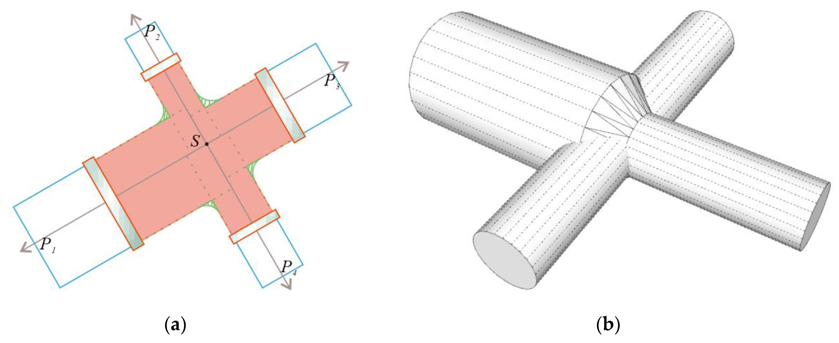
When multiple pipe segments intersect in a point, they are usually connected by a pipe joint, such as a tee-junction and cross-junction. For this complex situation, we use the parametric modeling method to adjust the model elements, including the pipe diameter and angle, to fit the pipe segments. Then, we combine multiple model elements to form a multi-pass structure. Figure 8 illustrates the composition of the multi-pass structure in top and oblique views.
The multi-pass modeling method involves two parts: (1) selecting the maximum diameter of multiple connected pipes as the standard for modeling the middle part; (2) build a cone between the larger and smaller pipe segments to realize a transition effect, as illustrated in Figure 8b. The parameters used here include the diameter of each pipe segment and adjustable transition length at the connection.

2.5. City-Scale Pipe Model Organization

As a city contains large amounts of pipe networks, the 3D scene cannot load and display all contents simultaneously; hence, block loading is required [25]. 3D Tiles is an open specification for streaming and rendering massive amounts of 3D geospatial content such as photogrammetry, 3D buildings, BIM/CAD, enhanced features, and point clouds. It defines a hierarchical data structure and a set of tile formats that delivers renderable content. 3D Tiles is built based on the GL Transmission Format, which is recommended by the Open Geospatial Consortium [26,27]. This specification is supported by 3D engines such as Open Scene Graph (OSG) and Cesium. The pipeline model partitioning principle should consider that pipe segments should not be segmented. Therefore, pipelines should be partitioned at pipe points to avoid cutting the pipe segment. To achieve this goal, we improved upon the common quadtree partition rules, in such a way that child tiles overlap but spatial coherence is still preserved, a parent tile encloses all of its children, and the tiles at the same level of the tree can have different sizes. This is a variation of quadtree, named loose quadtree in this study. The approach is useful for pipe network visualization to avoid splitting pipe segments and pipe-point models.

2.5.1. Data Organization for Pipe Model in 3D Tiles

For pipeline model creation, the model data are organized according to the 3D Tiles specification. The core element of 3D Tiles is a tileset file. A tileset is a set of tiles organized in a hierarchical structure. The tileset is described in JavaScript Object Notation (JSON), which is a lightweight data-interchange format. Figure 9 displays a simple example of a tileset to show its most important concepts and elements. To maintain a balance between visualization effectiveness and efficiency, level of detail (LOD) technology is adopted to construct models with different details at various levels. The pipe model generated by the parametric modeling algorithm is adopted in the tileset as a batched 3D model. The prototype models constituting the pipe point model are the same, but the corresponding spatial positions vary. For example, the water valve adopts the same model in the model library in the pipe point modeling process; to avoid being loaded multiple times during rendering, it is loaded as an instanced 3D model. Regardless of how many references there are, only one copy is stored in memory.

2.5.2. Splitting Pipe Models into 3D Tiles

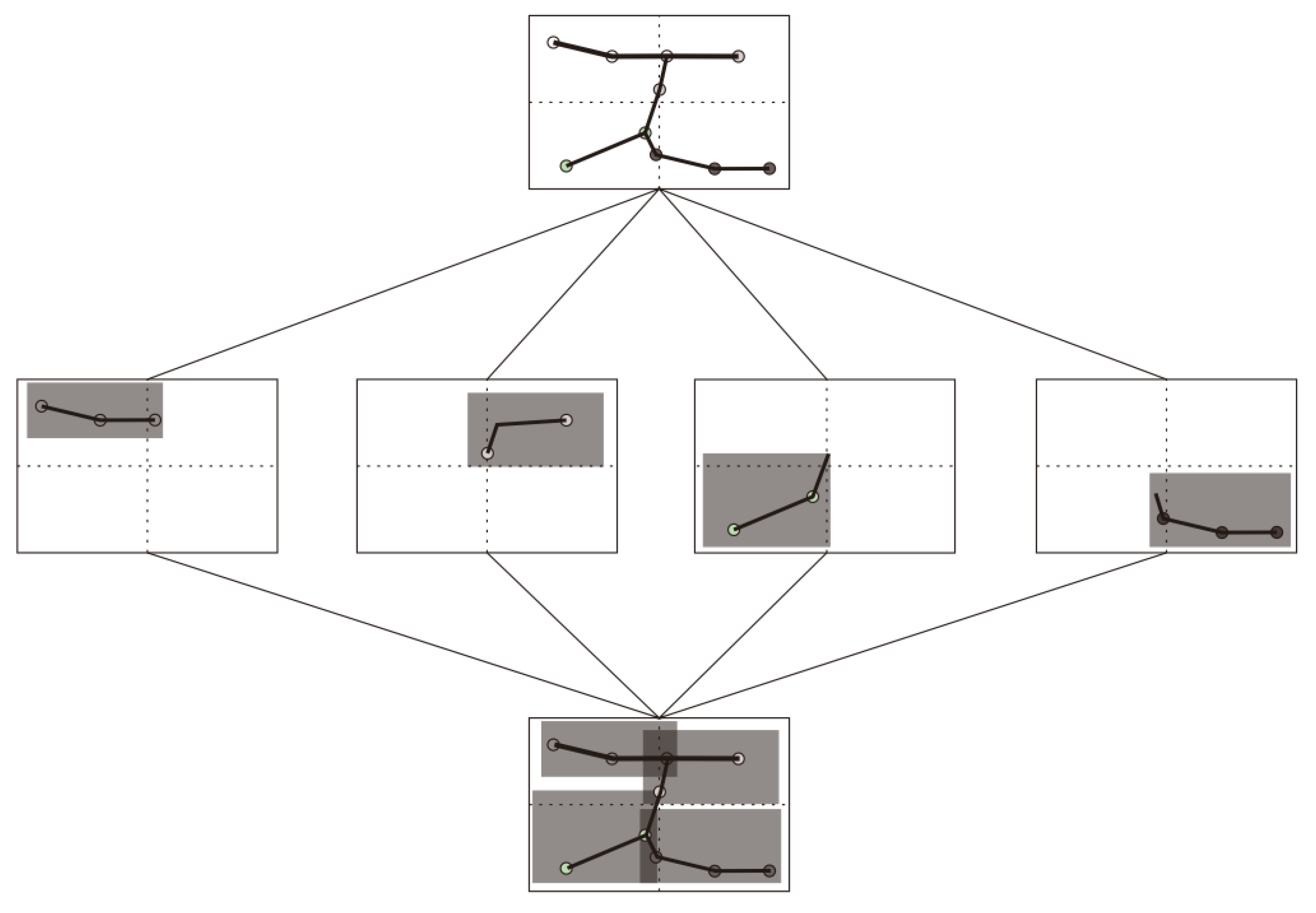
3D Tiles incorporate the hierarchical LOD(HLOD) concept to optimally render spatial data [28]. A tileset of 3D Tiles is a set of tiles, which are organized as a hierarchical data structure. The tileset itself contains the root tile, and each tile may have child tiles. The conventional quadtree organization method cannot meet the demands of pipeline division [29]; hence, we adopted a loose quadtree division method. For loose quadtree, the model will be completely split into the tile if the pipe-point model is at the boundary of the tile (Figure 10). At the same time, it will be marked that the model has been counted, and it will not be considered in the calculation of adjacent tiles. Hence, the tile size will be recalculated based on all models included, and finally a quadtree with loose structure will be formed.
For fast rendering, pipe segments and points can be split into tiles using the loose quadtree organization method. During the data conversion process, the format conversion function is integrated to transform the model data from the scattered OSG binary (OSGB) format to quadtree tiles, and then it is loaded into a 3D visualization engine for rendering.

3. Experiment and Analysis

To verify the proposed method, the pipe network data of a certain region in Beijing, China were selected for verification. As OSGB is a wildly used 3D model data format [30], an OSG-based tool was developed for parsing the MDB data and constructing pipe network models, and then the processed 3D Tiles data were loaded into Cesium to verify the visualization effect of the algorithm. The experimental environment was a 64-bit Windows 10 Professional operating system. The Central Processing Unit (CPU) was a 1.8 GHz eight-core Intel Core i7-8565U CPU with 16 GB of Random Access Memory (RAM), and the graphics card was an NVIDIA GeForce MX 150 with 2 GB of RAM. The screen resolution was 1920 × 1080 pixels, and the browser was Chrome 78.0.3904.108.

3.1. Experimental Data

In the experiment, integrated pipeline data were archived in a personal geodatabase using the MDB format. The pipeline data were divided into two parts. One contained four types of pipes with large diameters, i.e., water, drainage, gas, and heat supply in the urban area. The other part included the detailed pipeline information of a residential area. This experiment included seven types of pipelines. Table 3 displays the pipeline data statistics.

3.2. Performance

Based on the method proposed in this study, the pipeline data were first parsed. Then, the geometric model of the pipe network was generated by applying the parametric modeling method. Finally, the model data was formatted into 3D Tiles data according to the loose quadtree organization.
Table 4 displays the storage and time consumed by different experimental pipeline data types. The total storage of the standard model data (OSGB) is 1436 MB, and the total storage of the final 3D Tiles data (B3DM) is 1051 MB. As each line model type is independent, multithreaded parallel computing can be used [31]. The time consumed for the final model generation was 213 s, and the time for converting OSGB to 3D Tiles was 182 s.
Figure 11 displays the parametric modeling results for several essential pipe points. Figure 11a presents the visual effect of the elbow of the water supply pipeline. Figure 11b illustrates the visualization effect of the hand-hole well model and communication pipeline. Figure 11c visualizes the tee point of the rainwater pipeline, including the rainwater well and grate. Figure 11d displays the cross of the gas pipeline in a residential area.
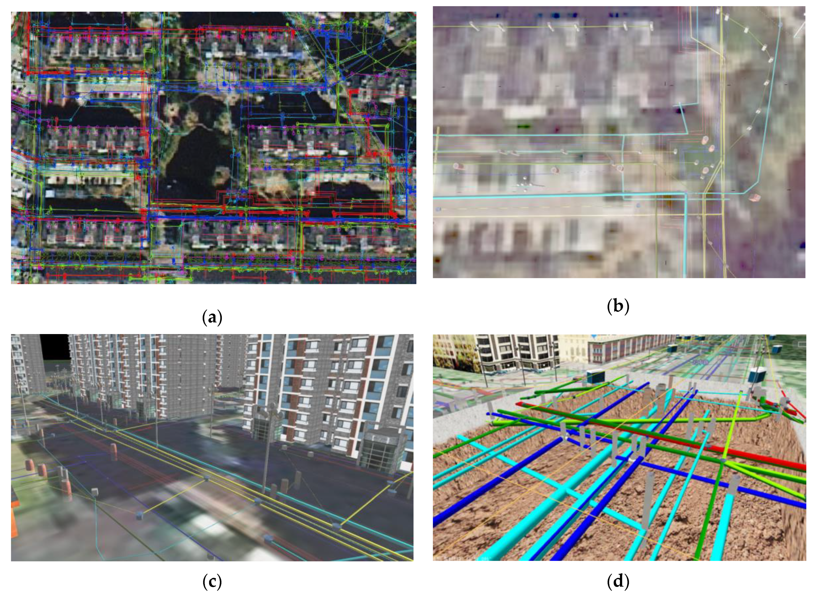
Figure 12 shows the visualization of large-scale pipe networks. The distribution of pipe networks in a large area can be rendered in the pipeline visualization system through the loose quadtree organizational structure. Figure 12a is a top view that demonstrates the rendering effect of the pipe network on a large scale. With the application of LOD technology, the pipeline model precision can be more effectively controlled, and the unnecessary consumption of computing resources can be avoided. Figure 12b displays the pipeline distribution at the road level, and the spatial distributions of different pipe networks can be observed. The combined rendering effect of the pipe network and buildings is presented in Figure 12c. Using a semi-transparent surface treatment and terrain-cutting algorithm, we can investigate the spatial distribution of the underground pipe network (Figure 12d).
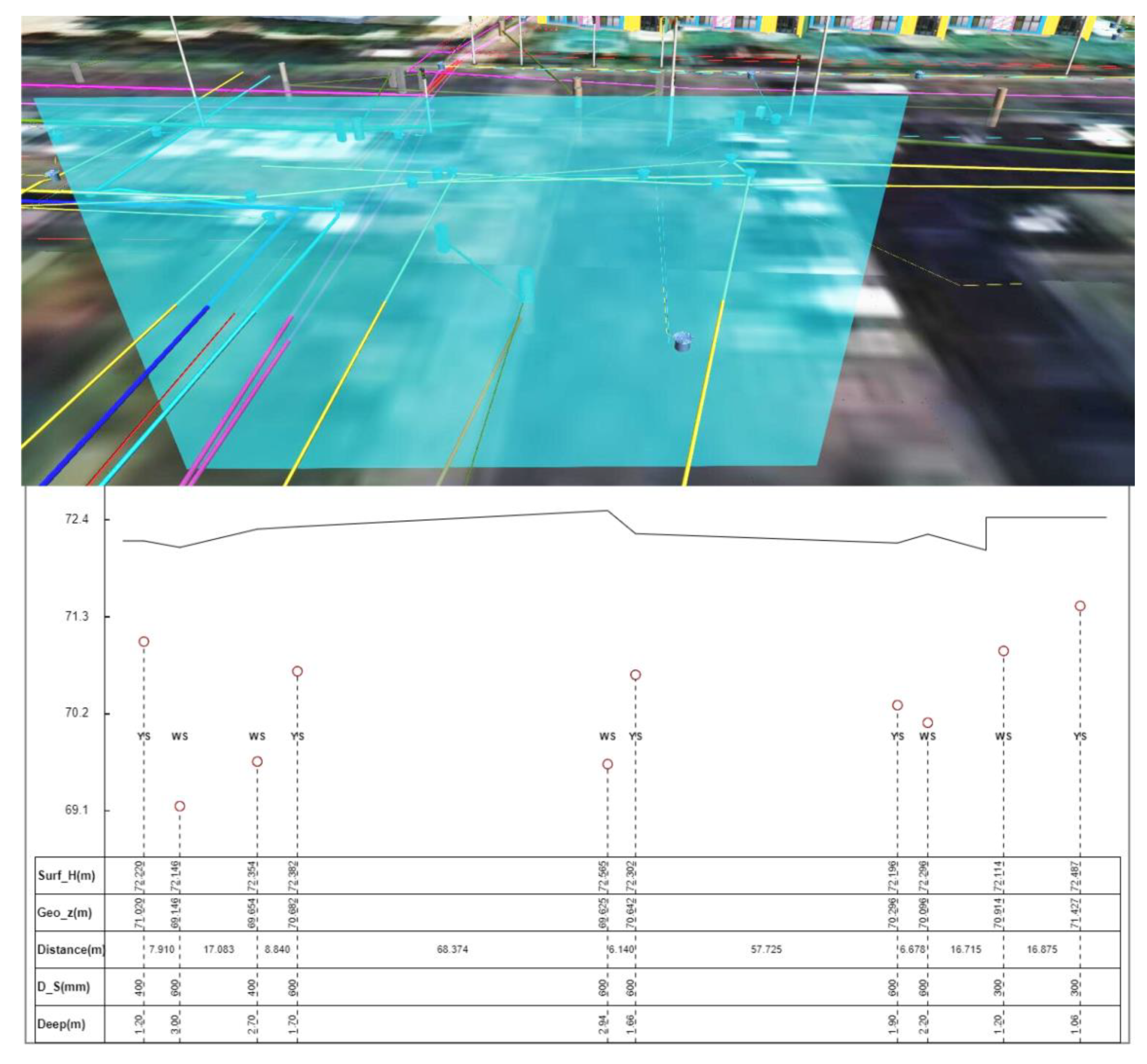
Figure 13 illustrates the pipeline section analysis, where the pipe diameters of underground pipe networks and the horizontal as well as vertical relationships between pipes are shown. The circle connected by a dotted line at the lower part of the figure indicates that the pipeline is round, and the corresponding surface elevation, buried depth, pipeline type, pipe diameter and distance between adjacent pipelines are shown at the bottom of the figure. At any two points on the map, the cross-section of the pipeline can be obtained. Through the section diagram, the buried depth of each pipeline and the distance between the pipelines can be clearly presented. For urban management, the distribution of pipe networks can be visualized before ground excavation [32] to avoid pipe networks breaking during the construction process.

4. Conclusions and Future Work

This study presents a pipe modeling and organization method for city-scale pipe visualization based on Cesium. The characteristics of pipe segment and point are considered to adopt a loose quadtree structure, making it possible to view a large range of pipeline data on a web browser. A 3D pipeline model can be quickly built using the parametric modeling method, and the pipeline connection can be constructed using the method mentioned in Section 2.3.1 to avoid cracks between pipeline segments. Different pipe point models were considered and processed, and the prototype model was automatically matched based on feature points. The pipe-point component model was generated based on the parameterized construction algorithm. For complex pipe points formed by several pipes with different diameters, the algorithm combined the flange model with a triangular mesh. After pipe network modeling, for quick browsing in Cesium, a format transformation from the original OSGB format to the B3DM format was performed, and the model data were organized into the 3D Tiles format through loose quadtree structure. Finally, a web-based 3D visualization system of pipeline networks was established, and the data modeling and processing workflows of different pipelines were validated. The approach has the following characteristics:
(1)
Pipe GIS data, including pipe segments and points, can be quickly and automatically processed into a 3D pipe model;
(2)
The pipe model is organized as a loose quadtree structure that can satisfy the visualization of city-scale underground pipe networks on a virtual globe.
As the pipe model is constructed using a geometric surface, internal pipe visualization and analysis are difficult to achieve. In smart city development, a detailed pipe model is essential for the urban emergency response. In the future, the internal and external integration of 3D pipe galleries should be investigated.

Author Contributions

All the authors contributed extensively to the work presented in this paper, Zihe Hu formed the research idea, designed and conducted the experiment, and drafted the manuscript. Jing Guo revised the manuscript and provided the financial support. Xuequan Zhang performed the experiment. All authors have read and agreed to the published version of the manuscript.

Funding

This research was funded by National Natural Science Foundation of China, grant number 41974035, and the Yong Elite Scientists Sponsorship Program by China Associate of Science and Technology, grant number 2018QNRC001.

Acknowledgments

The authors thank the Egova Co., Ltd. for providing data used for experiments.

Conflicts of Interest

The authors declare no conflict of interest.

References

  1. Mendez, E.; Schall, G.; Havemann, S.; Junghanns, S.; Fellner, D.; Schmalstieg, D. Generating semantic 3D models of underground infrastructure. IEEE Comput. Graph. Appl. 2008, 28, 48–57. [Google Scholar] [CrossRef]
  2. Balogun, A.L.; Matori, A.N.; Lawal, D.U. Geovisualization of sub-surface pipelines: A 3D approach. Mod. Appl. Sci. 2011, 5, 158. [Google Scholar] [CrossRef]
  3. Urban Underground Pipeline Survey. Available online: http://www.mohurd.gov.cn/wjfb/201605/t20160510_227405.html (accessed on 10 March 2020).
  4. Döner, F.; Thompson, R.; Stoter, J.; Lemmen, C.; Ploeger, H.; van Oosterom, P.; Zlatanova, S. Solutions for 4D cadastre—with a case study on utility networks. Int. J. Geogr. Inf. Sci. 2011, 25, 1173–1189. [Google Scholar] [CrossRef]
  5. Hijazi, I.H.; Ehlers, M.; Zlatanova, S. Nibu: A new approach to representing and analysing interior utility networks within 3D geo-information systems. Int. J. Digit. Earth 2012, 5, 22–42. [Google Scholar] [CrossRef]
  6. Li, S.; Cai, H.; Kamat, V.R. Uncertainty-aware geospatial system for mapping and visualizing underground utilities. Autom. Constr. 2015, 53, 105–119. [Google Scholar] [CrossRef]
  7. Peng, J.; Peng, F. Le A GIS-based evaluation method of underground space resources for urban spatial planning: Part 1 methodology. Tunn. Undergr. Space Technol. 2018, 74, 82–95. [Google Scholar] [CrossRef]
  8. Hou, Z.; Gu, Q. An improved method for drawing point of underground pipeline in AutoCAD. J. Geomat. 2011, 4, 43–44. [Google Scholar]
  9. Liu, H.Y.; Small, J.C.; Carter, J.P. Full 3D modelling for effects of tunnelling on existing support systems in the Sydney region. Tunn. Undergr. Space Technol. 2008, 23, 399–420. [Google Scholar] [CrossRef]
  10. Du, Y.; Zlatanova, S. An approach for 3D visualization of pipelines. In Innovations in 3D Geo Information Systems; Springer: Berlin/Heidelberg, Germnay, 2006; pp. 501–507. ISBN 354036997X. [Google Scholar]
  11. Becker, T.; Nagel, C.; Kolbe, T.H. Semantic 3D modeling of multi-utility networks in cities for analysis and 3D visualization. In Progress and New Trends in 3D Geoinformation Sciences; Pouliot, J., Daniel, S., Hubert, F., Eds.; Springer: Berlin/Heidelberg, Germany, 2013; pp. 41–62. [Google Scholar]
  12. Gröger, G.; Plümer, L. CityGML—Interoperable semantic 3D city models. ISPRS J. Photogramm. Remote Sens. 2012, 71, 12–33. [Google Scholar] [CrossRef]
  13. Wu, Z.; Wang, N.; Shao, J.; Deng, G. GPU ray casting method for visualizing 3D pipelines in a virtual globe. Int. J. Digit. Earth 2019, 12, 428–441. [Google Scholar] [CrossRef]
  14. Clarke, R.J. Planning and mapping of underground space—An overview. Tunn. Undergr. Space Technol. 2000, 15, 271–286. [Google Scholar] [CrossRef]
  15. Hunter, J.; Brooking, C.; Reading, L.; Vink, S. A Web-based system enabling the integration, analysis, and 3D sub-surface visualization of groundwater monitoring data and geological models. Int. J. Digit. Earth 2016, 9, 197–214. [Google Scholar] [CrossRef]
  16. Resch, B.; Wohlfahrt, R.; Wosniok, C. Web-based 4D visualization of marine geo-data using WebGL. Cartogr. Geogr. Inf. Sci. 2014, 41, 235–247. [Google Scholar] [CrossRef] [Green Version]
  17. Cesium. Available online: https://cesiumjs.org/about/ (accessed on 29 March 2020).
  18. 3D Tiles. Available online: https://cesium.com/blog/2015/08/10/introducing-3d-tiles/ (accessed on 9 June 2020).
  19. 3D Tiles Specification. Available online: https://github.com/AnalyticalGraphicsInc/3d-tiles/tree/master/specification#tileset-json (accessed on 9 June 2020).
  20. Chen, Y.; Shooraj, E.; Rajabifard, A.; Sabri, S. From IFC to 3D tiles: An integrated open-source solution for visualising BIMs on cesium. ISPRS Int. J. Geo Inf. 2018, 7, 393. [Google Scholar] [CrossRef] [Green Version]
  21. Jurado, J.M.; Ortega, L.; Graciano, A.; Feito, F.R. Web-based GIS application for real-time interaction of underground infrastructure through virtual reality. In Proceedings of the GIS: Proceedings of the ACM International Symposium on Advances in Geographic Information Systems, Redondo Beach, CA, USA, 1–10 November 2017. [Google Scholar]
  22. Wang, S.; Sun, Y.; Sun, Y.; Guan, Y.; Feng, Z.; Lu, H.; Cai, W.; Long, L. A hybrid framework for high-performance modeling of three-dimensional pipe networks. ISPRS Int. J. Geo Inf. 2019, 8, 441. [Google Scholar] [CrossRef] [Green Version]
  23. China, M. Of H. and U.-R.D. of the P.R. of Technical Specification for Urban Underground Pipeline Detection. Available online: http://www.mohurd.gov.cn/wjfb/201905/t20190506_240463.html (accessed on 9 June 2020).
  24. Weinhaus, F.M.; Devarajan, V. Texture mapping 3D models of real-world scenes. ACM Comput. Surv. 1997, 29, 325–365. [Google Scholar] [CrossRef]
  25. Goodchild, M.F.; Guo, H.; Annoni, A.; Bian, L.; De Bie, K.; Campbell, F.; Craglia, M.; Ehlers, M.; Van Genderen, J.; Jackson, D.; et al. Next-generation digital earth. Proc. Natl. Acad. Sci. USA 2012, 109, 11088–11094. [Google Scholar] [CrossRef] [Green Version]
  26. Khronos Group Inc. glTF Overview. Available online: https://www.khronos.org/gltf/ (accessed on 6 June 2020).
  27. Keysers, J. Review of Digital Globes 2015; Australia and New Zealand Cooperative Research Centre for Spatial Information: Melbourne, Australia, 2015; ISBN 0994301901. [Google Scholar]
  28. Zinsmaier, M.; Brandes, U.; Deussen, O.; Strobelt, H. Interactive level-of-detail rendering of large graphs. IEEE Trans. Vis. Comput. Graph. 2012, 18, 2486–2495. [Google Scholar] [CrossRef]
  29. Ebdon, D. SPANS-A quadtree-based GIS. Comput. Geosci. 1992, 18, 471–475. [Google Scholar] [CrossRef]
  30. Wang, R.; Qian, X. OpenSceneGraph 3.0: Beginner’s Guide; Packt Publishing Ltd.: Birmingham, UK, 2010; ISBN 1849512833. [Google Scholar]
  31. Silc, J.; Robic, B.; Ungerer, T. Asynchrony in parallel computing: From dataflow to multithreading. J. Parallel Distrib. Comput. Pract. 1998, 1, 3–30. [Google Scholar]
  32. Li, X.; Yeh, A.G.O. Modelling sustainable urban development by the integration of constrained cellular automata and GIS. Int. J. Geogr. Inf. Sci. 2000, 14, 131–152. [Google Scholar] [CrossRef]
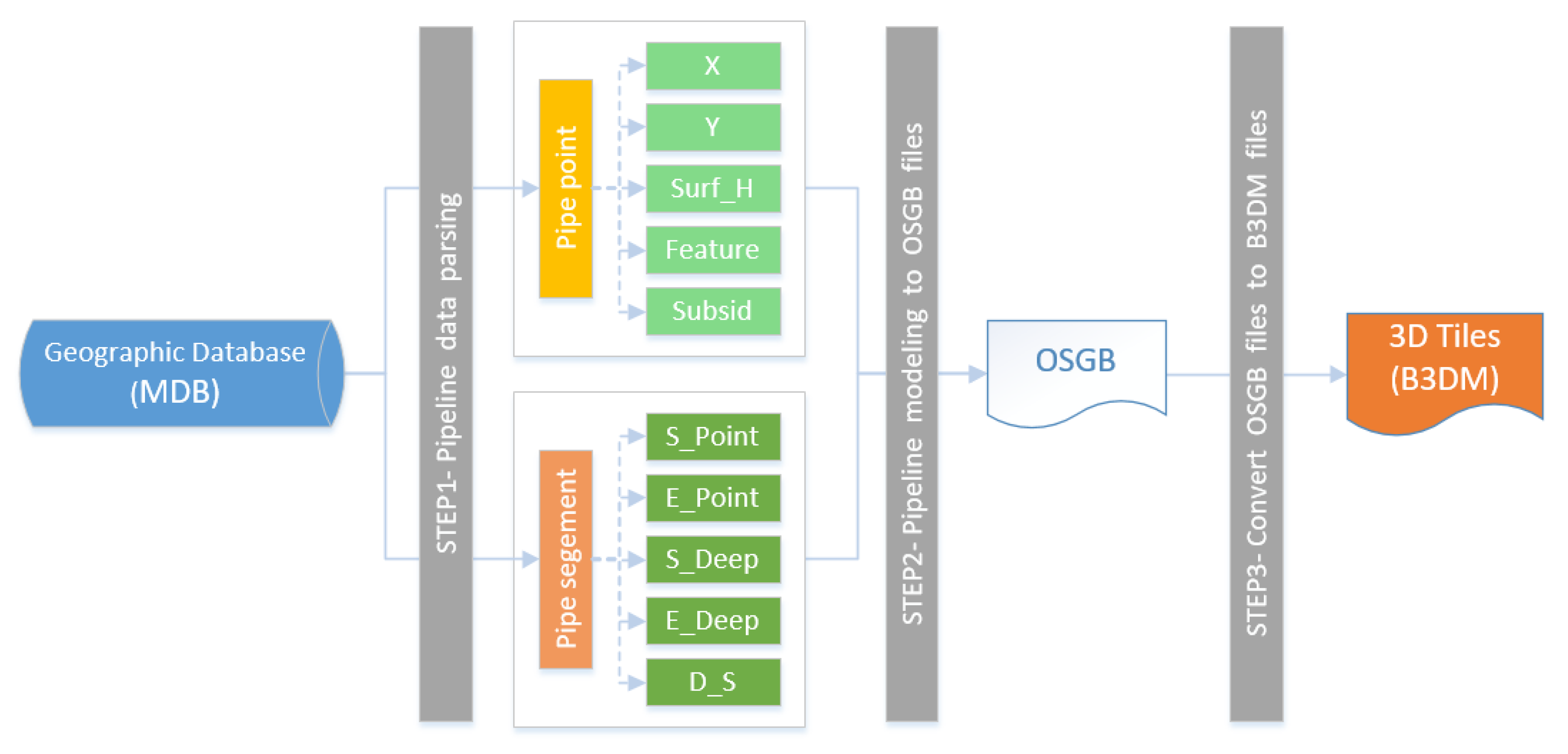
Figure 1. Flowchart of the pipeline data processing.
Ijgi 09 00623 g001
Figure 2. Illustration of underground pipelines using two pipe points: (a) cylinder pipe segment; and (b) rectangular pipe segment.
Ijgi 09 00623 g002
Figure 3. Connection of two pipe segments: (a) construction of suture for the crevice; (b) section of the suture.
Ijgi 09 00623 g003
Figure 4. Three-dimensional (3D) suture of two pipe segments.
Ijgi 09 00623 g004
Figure 5. Texture mapping of the pipeline suture.
Ijgi 09 00623 g005
Figure 6. Rotation diagram of pipe point model.
Ijgi 09 00623 g006
Figure 7. Flange on a pipeline elbow.
Ijgi 09 00623 g007
Figure 8. Multi-pass structure with four different diameter segments: (a) top view and (b) oblique view.
Ijgi 09 00623 g008
Figure 9. Pipe model data organization in 3D Tiles format.
Ijgi 09 00623 g009
Figure 10. Loose quadtree tile structure.
Ijgi 09 00623 g010
Figure 11. Visualizations of different pipeline connection types: (a) elbow; (b) hand-hole well; (c) rainwater well with water grate; and (d) pipeline cross.
Ijgi 09 00623 g011aIjgi 09 00623 g011b
Figure 12. Visualizations of the pipe network: (a) top view; (b) road-level view; (c) pipe network with buildings; and (d) semi-transparent surface.
Ijgi 09 00623 g012
Figure 13. Cross-section analysis of pipe network: the upper part shows the visualization of the cross-section in the 3D scene, and the lower part is the result of the cross-section analysis.
Ijgi 09 00623 g013
Table 1. Data fields for pipe point.
IDField NameMeaningComment
1Exp_NoNo. of pipe point
2XX coordinateSurveying coordinate systems
3YY coordinateSurveying coordinate systems
4Surf_HGround elevation
5FeatureFeature of pipe point
6SubsidSubsidiary type of pipe point
7AngleRotate angle of subsidiary
8OffsetOffset of eccentric well
Table 2. Data fields for Pipe segment fields.
IDField NameMeaningComment
1S_PointNo. of start point
2E_PointNo. of end point
3S_DeepDepth of start point
4E_DeepDepth of end point
5D_SDiameter of segmentLike D300 or 300 * 600
6MaterialMaterial of pipe segmentLike polyethylene or nodular cast iron
Table 3. Pipeline statistics.
TypeWater SupplyDrainageGasHeatingCommunicationsTelevisionElectricity
Number of pipe points55,29515,77720,79315,49110321281196
Length of pipeline (km)1191.9459.3472.2976.223.44.422.9
Table 4. Data conversion time and storage space.
Pipeline TypeOSGB SizeB3DM SizeGeneration TimeConversion Time
Water supply787 MB508 MB213 s182 s
Drainage149 MB136 MB45 s37 s
Gas146 MB126 MB42 s35 s
Heating273 MB213 MB89 s58 s
Communications10 MB17 MB4 s5 s
Television6 MB5 MB2 s4 s
Electricity65 MB46 MB23 s21 s
Publisher’s Note: MDPI stays neutral with regard to jurisdictional claims in published maps and institutional affiliations.