1. Introduction
Global Soil Map projects related to obtaining spatial soil information require new techniques for constructing soil maps that can use legacy data in digital soil mapping [
1,
2,
3]. Digital soil mapping is the process of creating and populating geographically referenced soil databases generated at specific resolutions via field and laboratory observation methods coupled with environmental data through quantitative relationships [
4]. This soil-mapping paradigm is based on the use of modelling methods for establishing the soil–landscape relationships needed to estimate the probability of soil occurrence or its properties described by environmental or remote sensing data [
5,
6,
7,
8,
9,
10].
The digital soil mapping paradigm is gradually replacing the traditional soil mapping paradigm; however, huge archives of traditional soil maps exist and were created by expert soil-mappers in accordance with the qualitative paradigm [
5]. To completely utilize these archives, digital soil mapping approaches should consider the qualitative nature of these traditional soil mapping processes. When utilizing legacy soil maps, it is most beneficial to use statistical methods that provide pedological knowledge in a form close to traditional forms [
11]. There should also be possibilities for extracting and exploiting traditional qualitative knowledge about spatial soil propagation in the statistical models in an objective form [
12,
13]. It is also important in digital soil mapping to adopt “sleeping beauty” ideas and techniques from the traditional processes of soil mapping [
14].
In traditional soil mapping, the values of other products besides soil maps are often underestimated. This product involves explicit rules for the delineation of soil class units or soil properties. These explicit rules were formulated by soil-mapping experts and have rarely been expressed in their complete form. These rules were evaluated by experts to determine their notional consistency and have been used to predict soil trends and investigate soil geography and many other applications. For digital soil mapping, qualitative knowledge can be incorporated into quantitative soil models to yield more accurate soil maps in soil geography. For example, alluvial soils are associated with the floodplains of rivers, whereas organic soils are associated with swamps and marshes. In addition to these models, such expert qualitative information could provide substantial improvements in the accuracy of soil maps [
15].
There are many soil mapping frameworks that are based on statistical methods and provide satisfactory prediction results: DSMART—resampled classification trees [
16]; SoilGRIDs—Random Forest, multiple linear regression, and ensemble methods [
7]; and DoSoReMi—Random Forest [
17], among others. If a complete sample set is used for modelling, ensemble methods, such as a Random Forest, yield the highest prediction accuracy [
18,
19,
20]. However, there are several basic limitations for obtaining accurate statistical models based on “pure” quantitative statistical approaches without using additional qualitative knowledge [
21]. In addition, extrapolation issues exist due to a dependence on the quality of spatial sampling and over-fitting [
20].
Few developments in digital soil mapping represent the soil mapping rules in an explicit form. One such approach uses SoLIM (Soil Land Inference Mode) technology, which is based on fuzzy logic [
22,
23]. This approach differs from the traditional method of formulating rules for soil mapping. In 2003, Qi and Zhu developed another approach for formulating tree-based rules like traditional soil mapping using the See5 algorithm [
11]. Subsequently, this algorithm was integrated with the statistical fuzzy-logic approach [
24]. Therefore, the SoLIM framework integrates many traditional methods for soil mapping, enabling the development of pedologically sound soil maps.
Most existing frameworks integrate only some traditional methods for soil mapping. However, the traditional process of soil mapping compilation can be imitated using the achievements of digital soil mapping. Many useful results could be obtained if the entire work process of a traditional soil mapper was imitated, including the process of soil map compilation via the cartographic methods used for covariate analysis [
25]. In addition, there are approaches for incorporating expert knowledge into automatically created models, as well as extracting and transferring explicit knowledge [
26,
27,
28].
New approaches enable the combination of expert-based knowledge and mathematical modelling to fuse the quantitative and qualitative descriptions of the relationships between soils and soil formation factors. Structural equation modelling (SEM) is a contemporary approach that facilitates the integration of knowledge about soils into a statistical model and provides an opportunity to assess the inter-relationships of various soil properties during modeling [
21]. According to the authors, “It bridges the gap between empirical and mechanistic methods for soil–landscape modelling and is a tool that can help produce pedologically sound soil maps” [
12]. However, the SEM approach is more aimed at incorporating expert knowledge than extracting knowledge from legacy data. Moreover, full theoretical models of SEM are presently more complex than simply representing practical rules for soil delineation in the traditional soil mapping process.
Another method of extracting the soil–landscape relationship is to use methods based on classification and regression tree algorithms. Representation with decision trees involves using the practical rules that were considered by the soil-mapping experts for soil mapping. Philippe Lagacherie implemented one of the most widely used methods, the classification and regression tree algorithm, for soil mapping in 1992 [
29]. Feng Qi and A-Xing Zhu wrote a broad review about using the See5 algorithm to acquire knowledge for soil mapping [
11]. Most of the classification and regression tree algorithms use locally optimal splitting criteria such as Gini or entropy for recursive stepwise partitioning [
30]. These methods are aimed at obtaining satisfactory prediction accuracies but not at developing an optimal model. This leads to the substantial overlearning of a tree. Such a tree can be large and have poor notional consistency for some rules while yielding satisfactory prediction accuracy for the key site. These locally optimal methods include CART (Classification And Regression Trees), CTREE (Conditional Inference Trees), CHAID (Chi-square Automatic Interaction Detection), See5, and CUBIST (Rule- And Instance-Based Regression Modeling), along with many others [
31]. Classification and regression tree algorithms of a new type have been proposed and aim at finding the optimal and most meaningful classification trees, e.g., evolution trees [
31], neural decision trees [
32], and deep neural decision trees [
33]. Such globally optimal methods potentially allow much more meaningful knowledge to be obtained about the relationships between soil and soil formation factors.
Intrinsically, the methods for the extraction of soil–landscape relationships may only yield reliable models when the input data for modelling are available with good quality. In traditional soil mapping, soil mappers utilize a limited number of the most significant soil formation factor maps to formulate compact and comprehensive rules for soil delineation. The same strategy of using only meaningful covariates forms the basis of our approach that we propose for constructing meaningful statistical models that can be easily analyzed by experts [
15,
25,
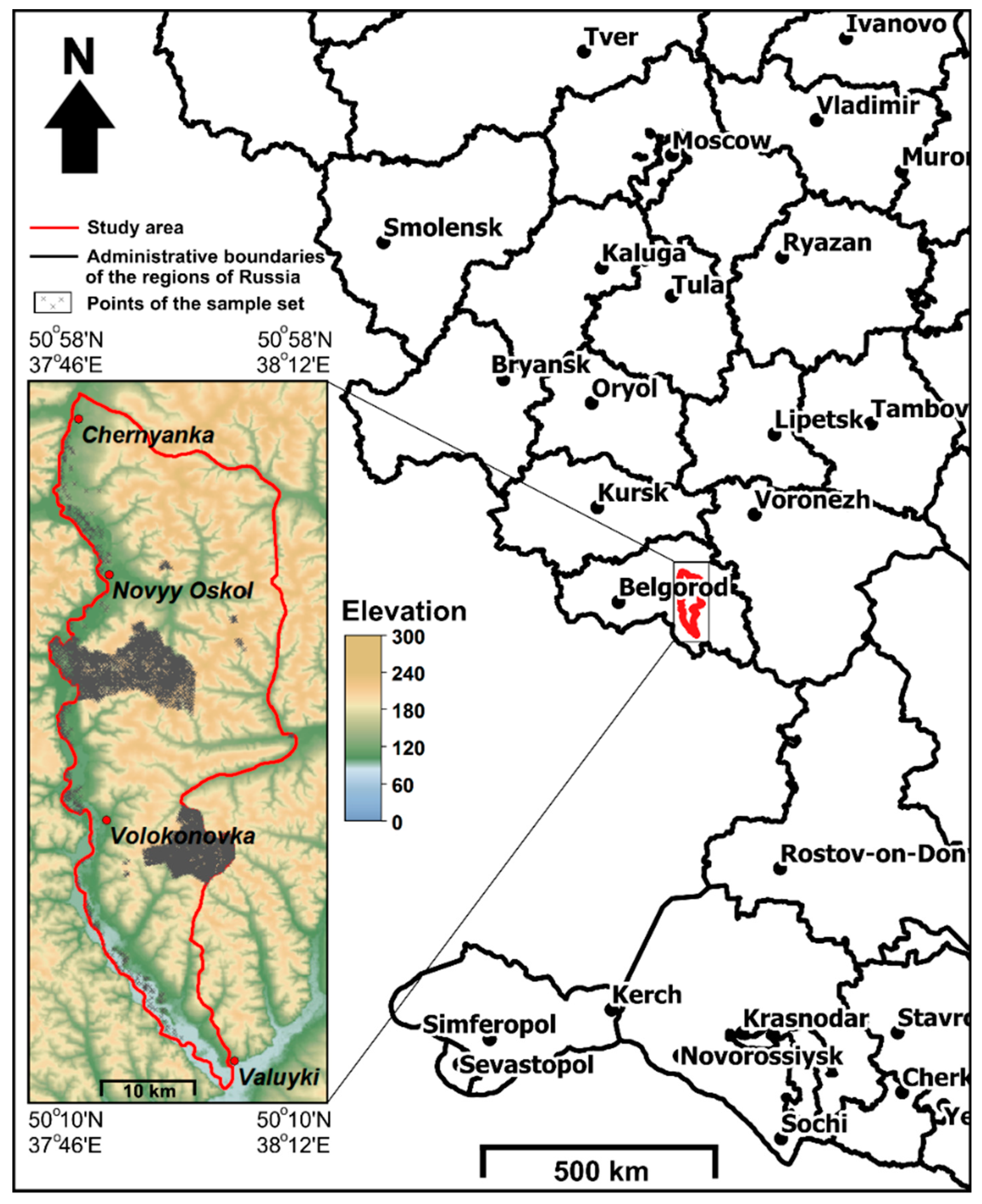
34]. In this study, we propose and evaluate a framework for constructing regional soil maps based on a digital imitation of traditional soil mapping and test this approach at a site in the Belgorod region of Russia.
3. Results
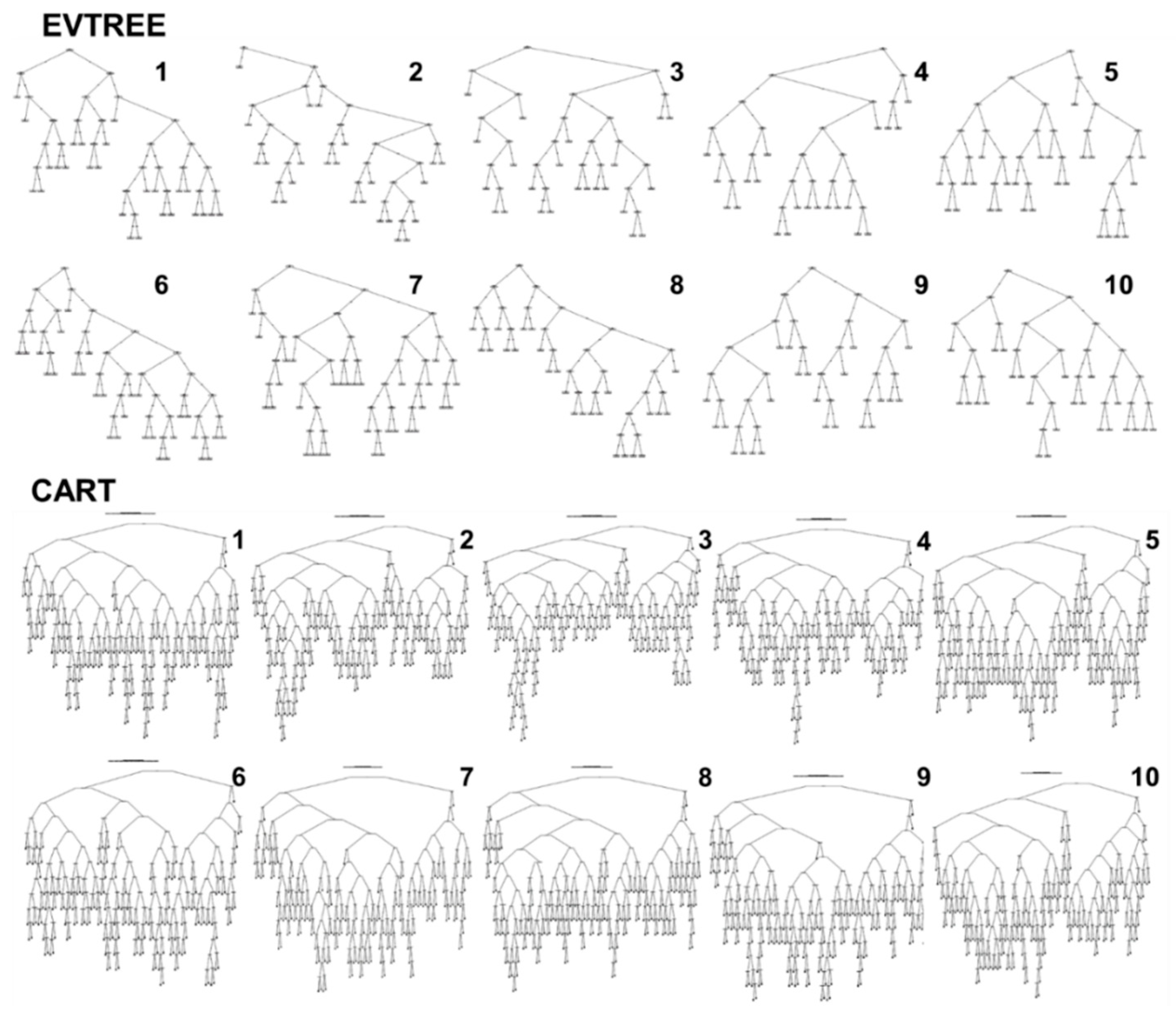
Decision trees with rules for soil delineation were created via the EVTREE and CART methods (
Figure 5). All trees that were produced by EVTREE were of a similar size; the trees that were produced by CART were also of a similar size, and the trees that were produced by EVTREE were more compact than the CART trees. Moreover, the decision trees that were created by EVTREE had different sequences of similar rules for soil class delineation (
Figure 5). All EVTREE trees, despite their formally different structures, presented similar relationships. The decision trees created by CART had similar rules for soil class delineation and similar sequences in the top part but different rules in the bottom part and, consequently, different sets of rules for soil class delineation.
The next example of rules for soil delineation is expressed in text form as follows:
3_G23—Grey and Dark Grey forest/Greyic Phaeozems Albic:
EVTREE_№5: (1) DEM_md15 < 203 m ^ RIVDIST >= 454505 m ^ DEM >= 171 m ^ LNDCVR = 45_Foret ^ DEM_md15 >= 203 m ^ 3_G23 (Probability: 12/15); (2) DEM_md15 >= 203 m ^ RIVDIST >= 333451 m ^ RIVDIST >= 371027 m ^ LNDCVR = 3_Water, 4_Leaf_Forest ^ 3_G23 (Probability: 47/58).
CART_№2: DEM < 171 m ^ RIVDIST < 337000 m ^ LNDCVR = 1_Grass, 2_Build_up_soils, 3_Water, 5_Coniferous_Forest ^ DEM_md15 < 203 m ^ (1) RIVDIST <= 539000 m ^ 3_G23 (Probability: 35/37); (2) DEM_ < 208 m ^ 3_G23 (Probability: 19/24); (3) DEM ->= 208 m ^ FLOWDIR = 2_E, 3_SE, 7_NW ^ 3_G23 (Probability: 4/10).
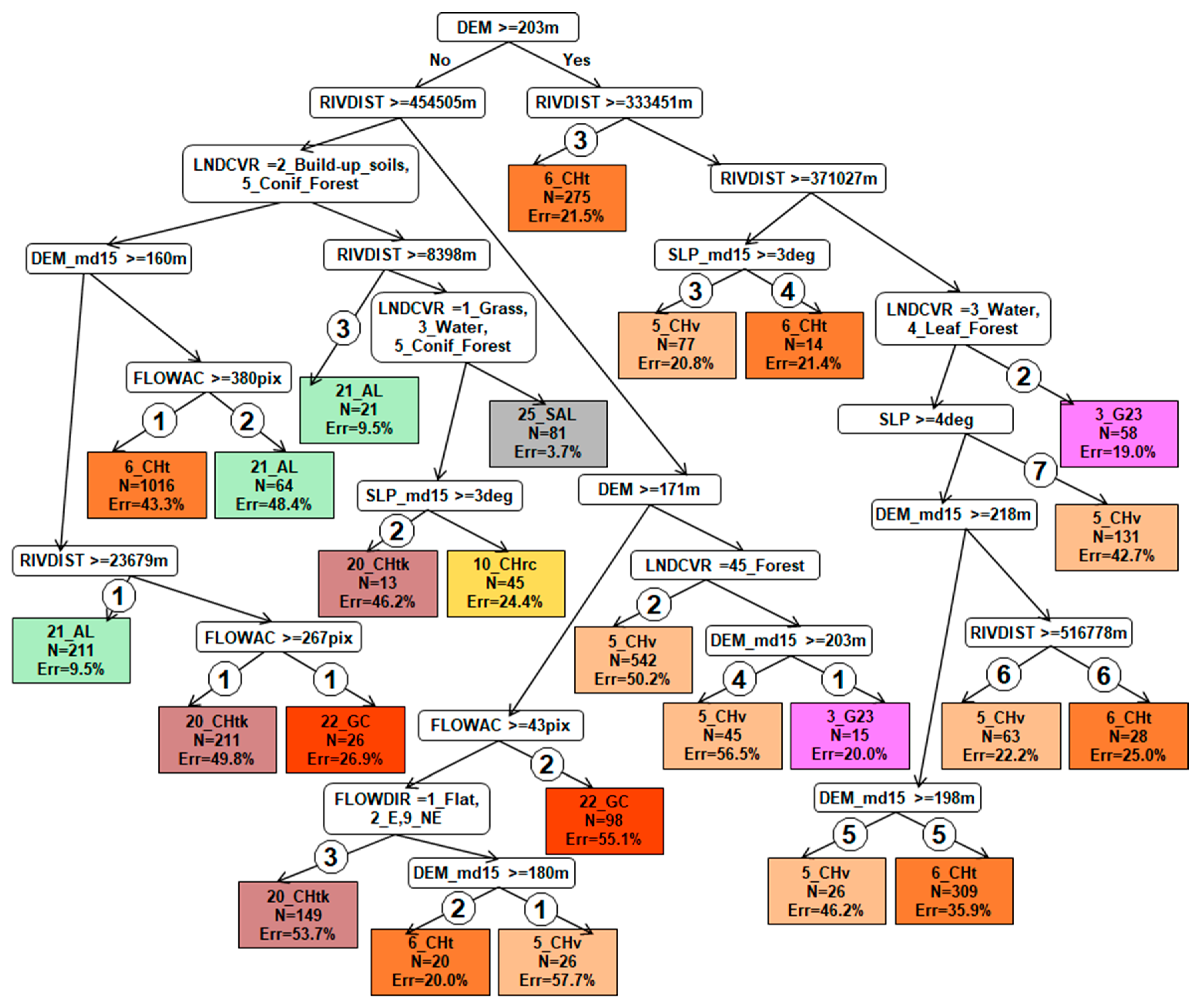
Description: EVTREE created branches for Phaeozem delineation in forests far from floodplains, where only leaf forests exist (
Figure 6). CART created many branches with various elevation derivatives, including elevations, slopes, and flow directions. Hence, the rules for Phaeozem delineation were overlearned by CART.
Another example of the rules for soil delineation is expressed in text form as follows:
21_AL—Alluvial Meadow/Umbric Fluvisols Oxyaquic:
EVTREE_№5: DEM < 203 m ^ RIVDIST < 454,505 m ^ (1) LNDCVR = any except 2_Build-up_soils or 5_Coniferous_Forest ^ DEM_md15 < 160 m ^ RIVDIST < 23,679 m ^ 21_AL (Probability: 191/211); (2) LNDCVR = any except 2_Build-up_soils and 5_Coniferous_Forest ^ DEM_md15 >= 160 m ^ FLOWAC < 380 pixels ^ 21_AL (Probability: 33/64); (3) LNDCVR = 2_Build-up_soils or 5_Coniferous_Forest ^ ^ RIVDIST < 8398 m ^ 21_AL (Probability: 19/21).
CART_№2: DEM < 171 m ^ RIVDIST < 9305 m ^ 21_AL (Probability: 190/200); (2) DEM < 171 m ^ RIVDIST >= 9305 m ^ LNDCVR <> 1_Grass, 45_Mixed_Forest, 3_Water, 4_Leaf_Forest ^ FLOWAC >= 68 ^ FLOWDIR = 2_E, 8_N, 9_NE ^ DEM_md15 < 156 m ^ FLOWDIR = 2_E, 9_NE ^ RIVDIST < 212,000 m ^ DEM_md15 > 120 m ^ 21_AL (Probability: 3/10). Six other sets of rules for the delineation of Fluvisols (21_AL) were not included in the text because of their large size (more than eight branches). These sets were applied to the total number of 61 test points.
Description: EVTREE delineated most Fluvisols directly according to their elevations and distances to rivers weighted with slopes. These are the correct rules for Fluvisol delineation. The CART algorithm created many overlearned sets of rules that led to large areas of Fluvisols in the river terraces (
Figure 6). Delineations by Random Forest were not correct as large areas of Fluvisols were identified in the river terraces instead of the floodplains (
Figure 6). The rules for the delineation of Fluvisols obtained by EVTREE were much more direct than those obtained by CART.
The decision trees that were created using the evolutionary learning of globally optimal trees (EVTREE) had much higher notional consistency than the trees created using the classification and regression tree algorithm (CART).
The trees for the study area that were produced by EVTREE had 20–29 conditions in comparison to 142–162 conditions for the trees that were produced by CART (
Table 4). The mean and minimum prior probabilities were similar for both methods (
Table 4). The minimum prior probabilities were related to typical Chernozem soil in both the EVTREE and CART methods. Thus, the EVTREE models are much more compact, which facilitates their interpretation.
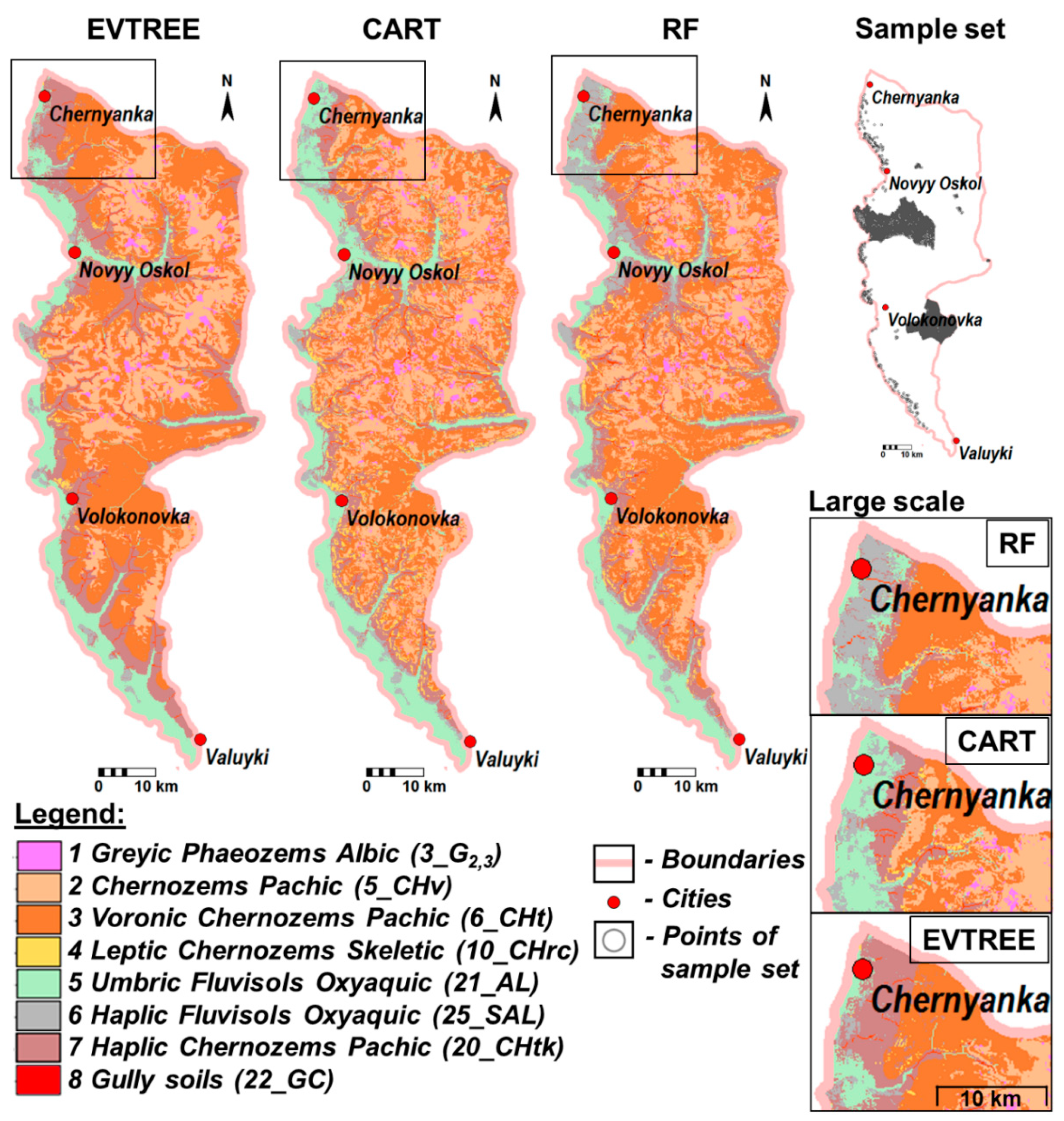
The soil maps were generally similar but exhibited some local differences (
Figure 7). Fluvisols were correctly mapped using only EVTREE as they were always associated with the rivers’ floodplains and not the rivers’ terraces or watershed areas. EVTREE selected the simplest rules for Fluvisols that gave the best accuracy. For soils with complex soil–landscape relationships, EVTREE offers less accuracy than CART. However, its method of selecting the simplest rules is much closer to the traditional approach.
The overall accuracy of the soil map created via Random Forest using the full sample set was 87% (
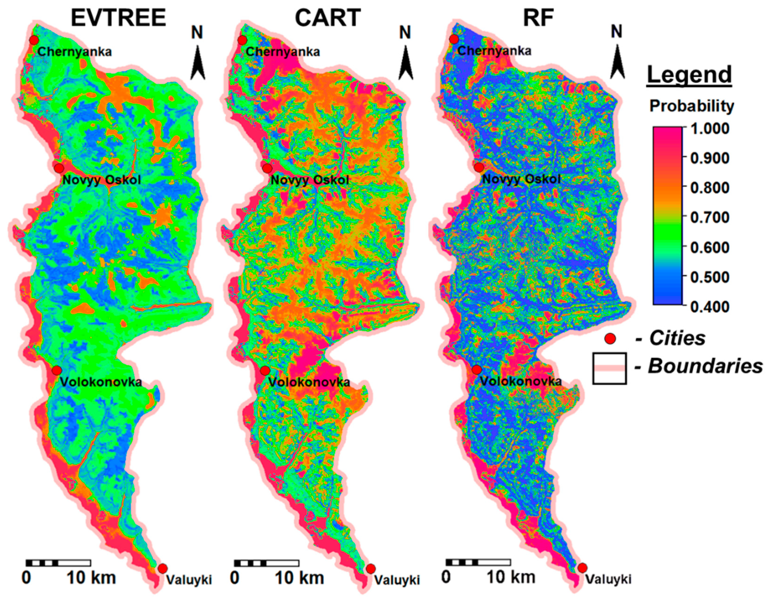
Table 5). Possibly, a part of the remaining 13% could be mapped using information about previous soil formation factors (soil formation factors such as the vegetation and climate that existed a thousand years ago could substantially affect the properties of soils but are not currently represented by covariates in digital soil mapping). The probability map created via the Random Forest algorithm demonstrated moderate quality, as the mean probability was 0.60 (
Figure 8). Despite the moderate quality of the model, Random Forest correctly predicted 87% of the independent test sample set. The CART probability map showed a high mean probability of more than 80% for large areas, while the real prediction accuracy was only 67%. As in other studies, the Random Forest model demonstrated the best prediction accuracy for the full sample set [
20].
The EVTREE probability map yielded moderate and high accuracy for watershed areas and floodplains, where the delineation of soils was easier. The lowest probabilities for EVTREE were observed for watershed slopes, where the delineation of Chernozem soils was not clear. For the Random Forest approach, the low accuracy on the probability map corresponded to occasionally satisfactory prediction accuracy, as measured by the test set, despite using many test points (approximately 2000 points). Therefore, only the probability map created by EVTREE was adequate. Notably, the limited number of covariates provided an advantage to EVTREE, while the approach using stochastic calculation of the probability map was not optimal.
After reducing the size of the training sample set from 5001 to 3304 points by reducing the squared areas with sample points (2 km
2), the accuracy remained the same for the CART and EVTREE methods, but for Random Forest, the accuracy decreased substantially by 20–30% (
Table 6). After increasing the mean distance between points by reducing the number of points from 5001 to 1785, the accuracy of all three methods decreased proportionally. When increasing the mean distance between points by reducing the size of the sample set to 1000 points, the Random Forest algorithm failed to run, and EVTREE and CART yielded similar accuracy to that used for 1785 points. For the small sample set, EVTREE and CART have an advantage over Random Forest because they can deal with a small number of cases.
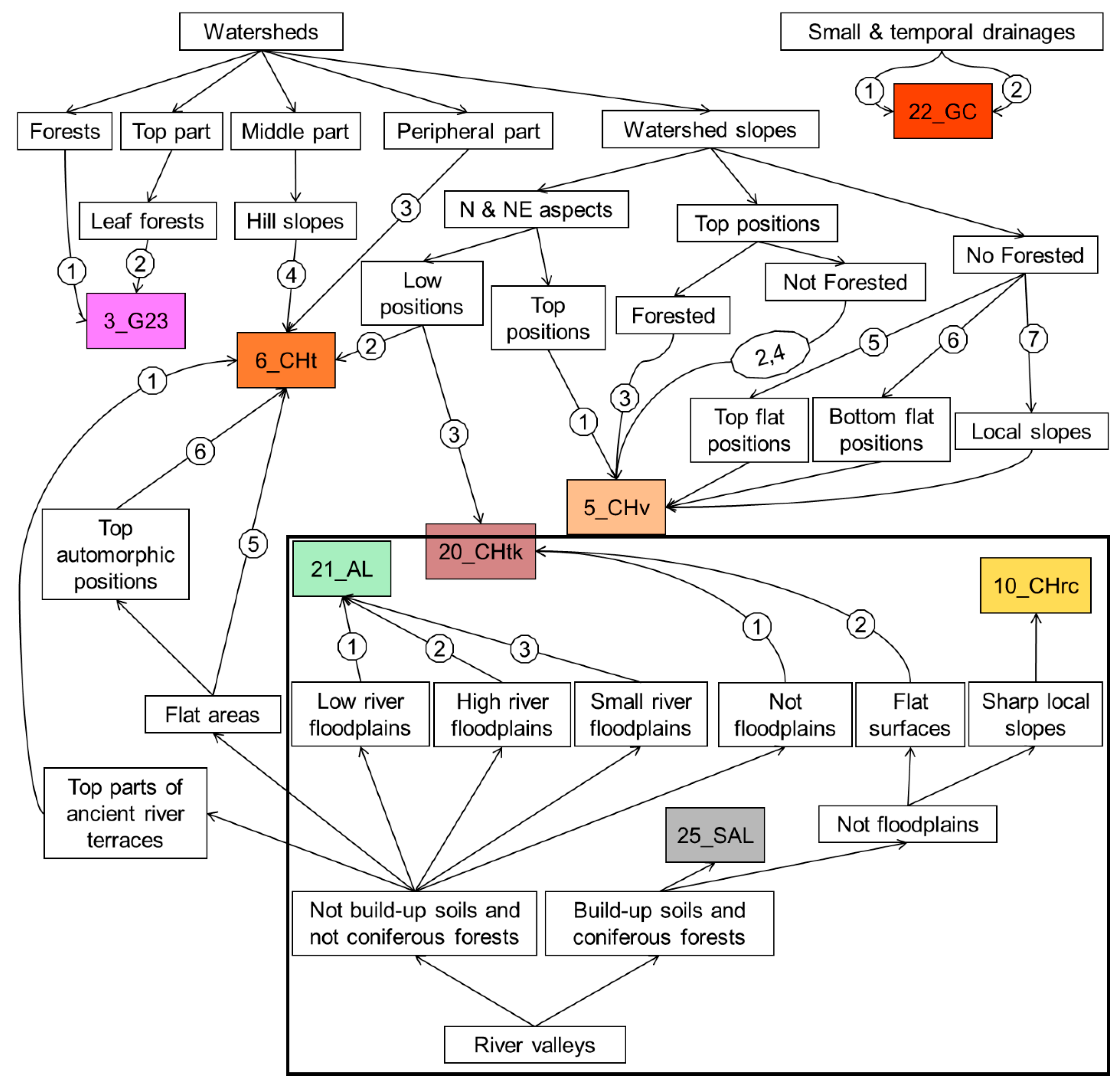
The decision trees obtained with the quantitative cartographic rules of soil unit delineation were analyzed to extract the real geographical qualitative relationships between the soil and soil formation factors, like those that were formulated via traditional soil mapping (
Figure 9).
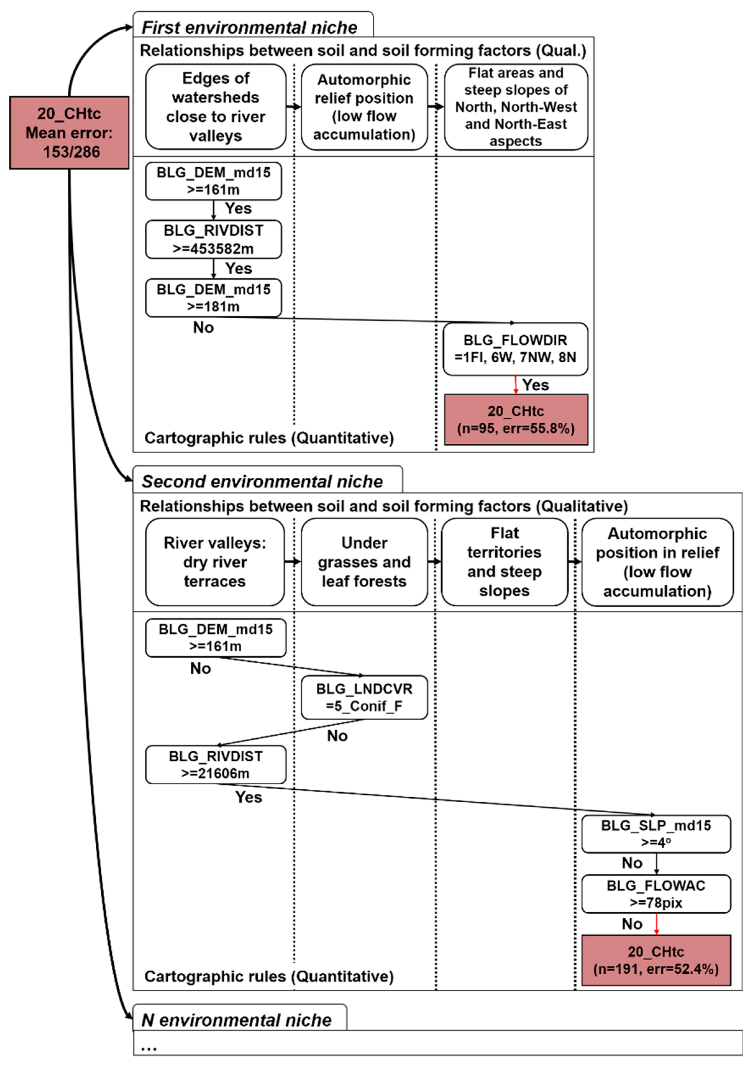
The obtained qualitative decision tree was represented in the form of separate rule chains for each soil. The rule chains were also split into environmental niches (
Figure 10).
Analysis of the soil delineation showed that
Fluvisols (21_AL) and
Gully complexes (22_GC) were not correctly mapped. This occurred because of the overly simplified river map, which led to a rough river distance map. The quality of the soil predictions can be improved by corrections of the soil formation factors maps. Consequently, we decided to rebuild the river distance map. We rebuilt the river and river distance maps using a parameter of river length equal to 100 m instead of 1000 m. This parameter represented the minimal length of a river on the map. Then we reran the EVTREE algorithm with the new input river distance map. In the resulting soil map, the visual difference between
Fluvisols (21_AL) and the
Gully complex (22_GC) soils was excellent. In the rebuilt tree, information about
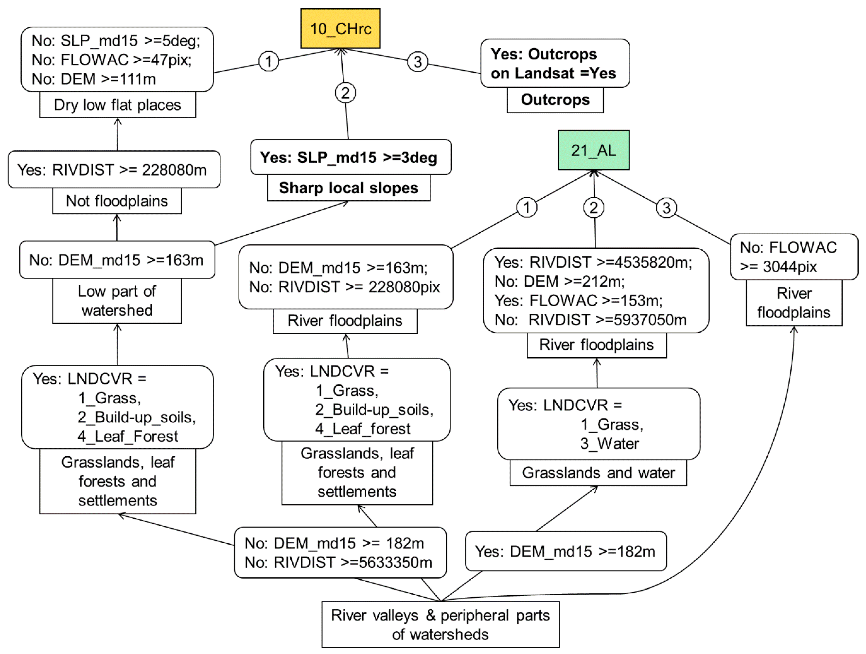
Chernozems calcareous soils (10_CHrc) was added. On the large-scale soil maps, these soils were mapped in the areas of outcrops. Such areas were recognized using Landsat satellite images and the supervised classification algorithm with the maximum likelihood method. For teaching, the original soil sample set for only outcrop areas was used. Then, the rule for accurately delineating
Chernozems calcareous (10_CHrc) soils in the areas of the outcrops was added to the classification tree (
Figure 11).
Therefore, there were at least four ways to correct the soil map:
An accuracy assessment was provided for the corrected soil map using another independent sample set of 1269 soil pits. The overall accuracy before manual correction was 65%, with 76% accuracy after correction. Therefore, based on soil geography knowledge, the covariates for the modelling and quantitative models were corrected by an expert to provide higher accuracy and notional consistency of the soil maps.
4. Discussion
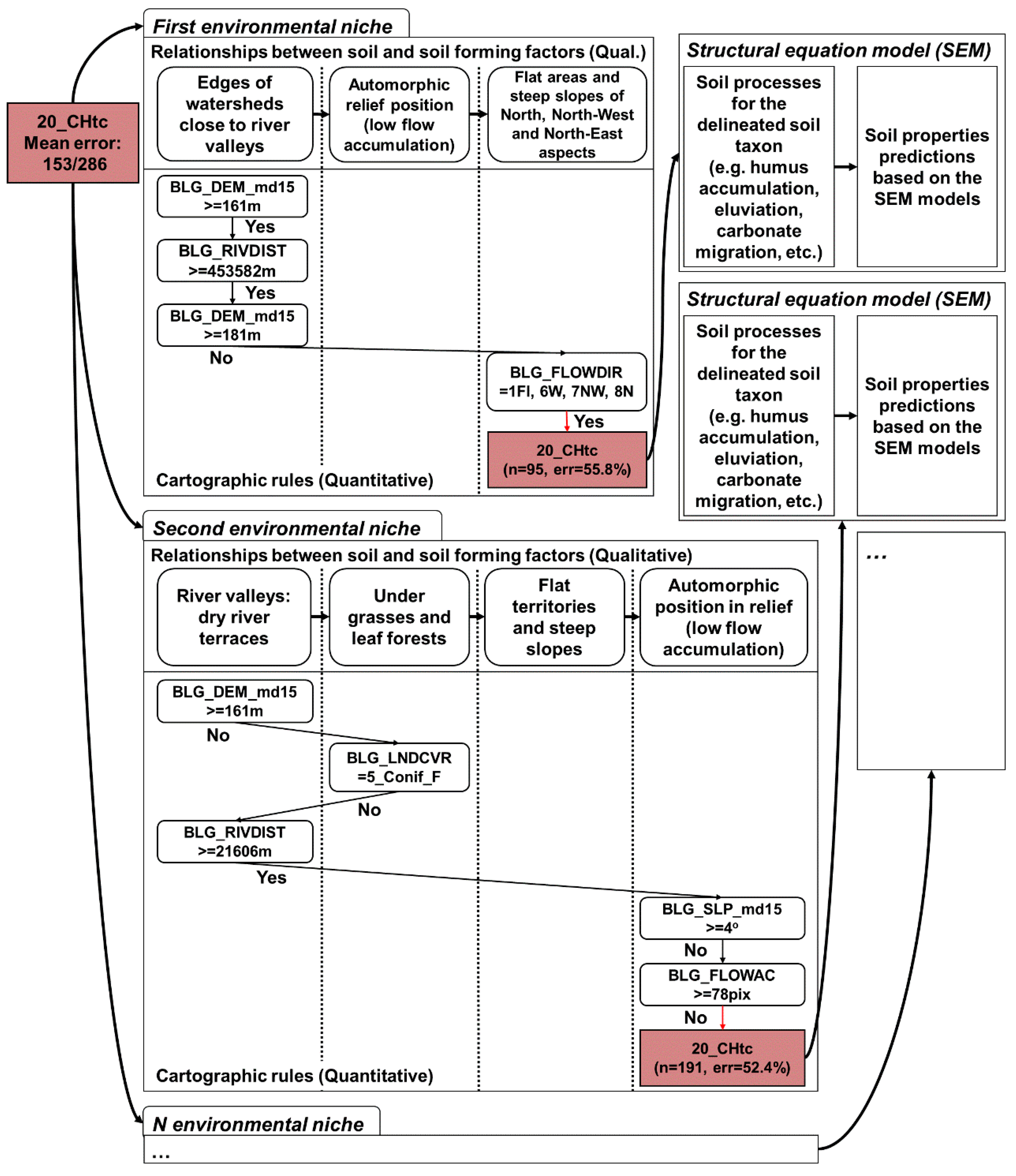
We obtained accurate soil maps automatically and made them much more accurate manually. The accuracy of the manually corrected soil map can reach one hundred percent, but this requires laborious work. The developed framework allowed us to implement the work of a traditional soil-mapper using the statistical method of evolutionary trees and the understandable representation of soil mapping rules. This statistical method was first used for digital soil mapping. The advantages of this method over the CART method are the compactness and reasonability of the model. The easy-to-use representation of soil–landscape relationships—as a decision tree and chains of rules—is an advantage of the proposed approach compared to structural equation modelling [
12,
21]. However, for mapping continuous soil properties, these two approaches can be used together. This process involves mapping soil units with classification trees and then splitting them into continuous soil property maps (
Figure 12).
This framework differs from the SoLIM because it aims at the development of approaches that fully imitate the work of a traditional soil mapper. Thus, the representation of the classification trees and rule chains was closely investigated. In our methodology, we used mostly traditional soil formation factor maps, such as geological parent materials and simple derivatives of the digital elevation model, rather than difficult indexes. We also used a traditional representative form of soil units instead of a fuzzy logic approach. Our framework and the package we developed provide a traditional soil mapping alternative to SoLIM [
22,
23]. Realization of this framework was strongly based on machine learning techniques and the advantages of the R statistical language, which make it congruent with the SoilGRIDs framework [
7].
The proposed forms of the relationships between the soil and soil formation factors, classification trees, and rule chains appear to be very convenient for interpretation. Qualitatively describing the quantitative rules was also simple, despite some subjective factors due to the expert nature of the analysis. Using mostly traditional soil formation factor maps helped us interpret the quantitative model and easily obtain the qualitative model. The obtained qualitative classification tree allowed us to visualize the complex environmental relationships for the study area in a form that is understandable for traditional natural scientists, soil scientists, geologists, ecologists, environmentalists, and others. This form is useful for environmental analysis, such as determining the reasons to change soils over time and defining the environmental state of the study area. This is a traditional type of analysis that is neglected in most other DSM methodologies. The soil mapping chains of the rule form were convenient for making the soil map and were manually corrected. This simple form can be programmed to make soil maps in most GIS programs. The novelty (associated with the chains of the rules) of our methodology compared to SoLIM is that our method uses groups based on environmental niches that are important for investigating the underlying reasons for soil geography. A considerable problem with our framework is the laborious work associated with the process of translating the relationships from the form of classification trees to rule chains. This process, however, can be automated and allowed us to collect important expert soil geography information.
Below we summarize the problems that we aimed to solve with the proposed framework.
The laborious manual work associated with producing two forms of soil rules as a general classification tree and soil-specific rule chains. A possible solution is using a package with an interface that allows one to make adjustments as easily as possible. Moreover, this method should permit automatic transformations between classification trees and chains of rules.
The significant changes in the classification trees when using updated covariate maps. This can be overcome by using more sophisticated statistical methods of finding classification rules and incorporating prior soil knowledge into the search for rules.
The mapping of soil classes when we need to map continuous soil properties or soil functions. Compliance with other methodologies provides a solution for this problem. In that case, the proposed framework offers an interface with legacy soil maps.
Statistical improvements of the classification tree algorithm’s accuracy.


