Spatial Distribution of China’s Industrial Output Values under Global Warming Scenarios RCP4.5 and RCP8.5

Abstract

Climatic changes significantly impact the socio-economic system. Compared with research on the impacts of climate change on the agricultural economic system, researches on the impacts on the industrial economic system are still scarce. This is mainly because of the difficulties in matching climate data with socio-economic data in terms of spatiotemporal resolution, which has greatly limited the exposure degree assessment and the risk assessment of industrial economic systems. In view of this, based on remote sensing inversion and multi-source data fusion, we generated kilometer-grid data of China’s industrial output in 2010 and built the spatial distribution model of industrial output, based on random forest, to simulate the spatial distribution of China’s industrial output under different climate change scenarios. The results showed that (1) our built spatial distribution simulation model of China’s industrial output under different climate change scenarios had an accuracy of up to 93.77%; (2) from 2010 to 2050, the total growth of China’s industrial output under scenario RCP8.5 is estimated to be 4.797% higher than that under scenario RCP4.5; and (3) the increasing rate of the average annual growth rate of China’s industrial output slows down significantly under both scenarios from 2030 to 2050, and the average annual growth rate will decrease by 7.31 and 6.54%, respectively, under scenarios RCP8.5 and RCP4.5 compared with that from 2010 to 2020.

1. Introduction

Since the 1980s, global changes, marked by global warming, have gradually been attracting significant attention worldwide [1]. Since climatic changes have considerable impacts on natural ecosystems and economic systems [2], coping with the impacts of global warming has become an important issue for all countries striving for sustainable development [3]. Against this background, measures to reduce greenhouse gas emissions are becoming increasingly important for the development of a sustainable industrial economy. Research on the impacts of climate change on the industrial economic system can directly or indirectly affect the sustainable development of global and regional economies as well as the development of climate adaptation measures and emission reduction standards. Hence, systematic research in this field is of great significance.

Among numerous socio-economic sectors, the industrial sector is highly sensitive to climatic changes, and its sensitivity ranks only behind that of the agricultural, aviation, and construction industries [4]. The impacts of climate change on the industrial sector are generally manifested in two aspects. The first one is the direct impact of climate change, especially in the form of extreme weather events, on industrial production [5]. Most of these impacts are negative, and extreme weather events can directly lead to infrastructure damage, production halting, and casualties in the industrial sector. The second aspect refers to the fact that climatic factors do not directly affect industrial production, but have potential indirect impacts on the industrial sector (e.g., processing industry, manufacturing industry) through agriculture and animal husbandry [6,7]. For example, climatic changes can result in increased or decreased agricultural production, thus affecting the price of agricultural products and, consequently, the costs of the processing and manufacturing industries that use these agricultural products as main raw materials. From another angle, demand and supply changes may also affect the industrial economy. For example, temperature rises can lead to a higher demand for air conditioners, electric fans, and cold drink products, which will promote the mass production and processing of such products. Several studies [8,9,10,11] have shown that, on a global level, extreme climatic events, such as heavy precipitation, drought, extremely high and low temperatures, have great positive and negative impacts on industrial economic systems, although the adverse impacts are dominant. Against the background of the predicted continuous climate warming in the future, industrial production will face several obstacles such as intensified resource exhaustion and frequent extreme climate events, resulting in a greater overall sensitivity to climate change.

At present, the exposure degree assessment on climate change mainly focuses on agriculture, forestry, husbandry, and the fishery industry [12]. Climatic changes can have direct impacts on the soil for agricultural production, resulting in altered crop growth. Related studies have shown that under the impact of climate change, the soil organic carbon (SOC) content in the top soil layer of Mediterranean agricultural areas generally decreases, while that in the lower soil layer generally increases [13]. For example, Awoye et al. [14] have investigated the impacts of climate change on the yields of different crops in western African countries and found that such changes could lead to a severe yield reduction of 11–33% for pineapple, corn, peanuts, cassava, and cowpea; whereas an average yield increment of 10–39% was calculated for sorghum, yam, cotton, and rice. At the same time, climatic changes can also have a serious impact on agricultural practitioners. Some studies have shown that due to the impact of climatic changes, the prevalence of diseases related to ultraviolet radiation and heat stress among agricultural workers presents an aggravating trend [15].

Although numerous studies have focused on the exposure degree of the primary industry [16,17,18], research on the exposure assessment of the secondary and tertiary industries is scarce. In the studies that identified the impacts of climate change on the industrial economic system, the core step is to conduct spatial superposition analysis on climate factor data and industrial data with the same spatiotemporal resolution [19]. However, at present, studies assessing industrial economic data mostly take the administrative divisions of cities and counties as the research unit, and such data can only be obtained in the form of average statistical data or aggregate statistical data, which cannot be matched with climate data on a spatial level. At the same time, the industrial economic data stored in the form of aggregate and average data cannot reflect the spatial heterogeneity of the industrial industry, resulting in a poor accuracy of climate risk assessments. Through quantitative description of the spatial distribution rules of grid-scale industrial economic data and the characteristics of grid-scale climatic changes, the mechanisms underlying the impacts of climate change on the industrial economic system can be revealed, thereby promoting research on the industrial economy against the background of climatic changes and climate risk assessment and providing a scientific basis for the proposal of policies to adapt to climatic changes and to mitigate their effects.

At present, research methods for the spatialization of economic data can be divided into three categories, i.e., the spatial interpolation model [20,21], the multi-source data fusion model [22,23], and the remote sensing inversion model [24]. Due to the premise of uniform distribution of social and economic data, the spatial interpolation model is mostly used in small-scale studies with large sample numbers, relatively flat terrain, and no other auxiliary data, whereas it is rarely used in large-scale studies where spatial changes are complex and data sampling is difficult. This is mainly because industrial output value data are generally stored in administrative regions such as provinces, cities, and counties. The spatial resolution is extremely low, and the spatialization accuracy of the spatial interpolation model is extremely poor, making it necessary to increase the number of sampling points; however, gathering statistics is difficult, and human, material, and financial resources are huge. The multi-source data fusion model aims to obtain accurate dependent variable results through correlation analysis or other analysis of multiple covariables. However, due to the autocorrelation between covariables and the heterogeneity of geographic space, the model should be implemented in partitioned subregions when large-scale regions are studied, which means that it has a poor universality. Due to the development of spatial data and remote sensing images [25,26], the multi-source fusion model is widely used. Compared with the spatialization by the interpolation model and the multi-source data fusion model, the nighttime light remote sensing data inversion model has a simple operation method, high accuracy, and spatiotemporal characteristics, potentially solving the problem of the spatialization of large-scale data. However, at present, this model is mainly applied in the analysis of GDP (Gross domestic product) and population data. In terms of industrial economy, due to the difficulty in the collection of statistical data, spatialized datasets for country-level and global industrial economy—especially spatialized datasets for the industrial economy under future climate scenarios—are scarce, impeding the risk assessment of the industrial economy.

In this context, the research objectives of this paper are as follows: (1) to explore the spatial distribution characteristics of industrial output at the current stage by taking mainland China as an example; (2) to analyze the changes in the industrial output under global warming scenarios RCP4.5 and RCP8.5, based on the random forest algorithm in machine learning.

2. Data Sources and Research Methods

2.1. Data Sources

In this paper, the definition of industry is based on the data statistical standards of the World Bank. Industry corresponds to ISIC (International standard industrial classification) divisions 10–45 and includes manufacturing (ISIC divisions 15–37); it comprises value added in mining, manufacturing (also reported as a separate subgroup), construction, electricity, water, and gas (

Table 1. Industrial sector and subsectors.

Industrial Sector
Mining and Quarrying	Manufacturing	Electricity, Water, and Gas	Construction
Coal and lignite mining, peat extraction, oil and gas extraction services, activities incidental to oil and gas extraction, etc.	Food and beverage manufacturing, tobacco products manufacturing, textile manufacturing, other transportation equipment manufacturing, furniture manufacturing, recycling, etc.	Electricity, gas, steam and hot water supply, collection, purification, and distribution of water	Construction

Note: Industry sector classification is based on World Bank and International Standard Industry Classification (ISIC) standards.

). The definition of the connotation of industry is as follows: divided into World Bank and the National Bureau of Statistics of China; industry includes mining, manufacturing, construction, power, water, and natural gas production and supply and excludes the construction industry from the industrial category. For global unification, and in accordance with the World Bank category, China’s industrial data is calculated according to the overall secondary industry.

Most of the data used in this paper were obtained from the Data Center of Resources and Environmental Sciences, Chinese Academy of Sciences, including administrative boundary data, industrial land use data, nighttime light remote sensing data, and other driving factor data. Meteorological data were derived from the China Meteorological Network and the coupled model Intercomparison Project Phase 5 (CMIP5). The statistical data were obtained from the China Statistical Yearbook, whereas vegetation data were derived from the MODIS (Moderate resolution imaging spectroradiometer) data.

All data used in the model were 1-km grid data (

Table 2. Data sources.

Data Category	Data Type	Year	Data Description
Land use data	Land use grid data	1990, 2000, 2010	Spatial resolution: 1 km
Meteorological data	Site data, multi-mode data	2000, 2010, 1850–2100	Temporal resolution: year
Vegetation data	EVI	2000, 2010	Temporal resolution: month
DEM	DEM	2010	Spatial resolution: 1 km
Economic data	Industrial output	2000, 2010	Temporal resolution: year
Driving factor data	Population, GDP, rivers, roads, urban settlements, rural settlements, urbanization rate	1987–2016	Temporal resolution: year

Notes: DEM is digital elevation model; EVI is Enhanced vegetation index; GDP is gross domestic product.

).

The Chinese physical geographic map with river and regional names is shown in Figure 1.

2.2. Research Methods

2.2.1. Research Design

The specific research design of this paper can be divided into four parts:

(1) Data collection and preprocessing

The acquired meteorological data, socio-economic data, nighttime light remote sensing data, and basic geographic data are preprocessed, including data clipping, data binarization, data rectification, and format transformation.

(2) Identification of climate change features

The ANUSPLIN model and the multi-mode fusion model are used to carry out interpolation operations based on the meteorological site data and CMIP 5 multi-mode data, and subsequently, the spatial distribution characteristics of climate factors in the study area under different climate scenarios in the past and future can be extracted.

(3)

In combination with the spatial data of the current industrial output value (2010), the spatial distribution of the current 1-km industrial output value is analyzed using the kernel density method.

(4)

Spatial distribution simulation of China’s industrial output under different climate change scenarios.

The industrial land use information from 2020 to 2050 can be extracted by the Logistic–CA–Markov model; which is a combination of logistic regression analysis, the cellular automata (CA) model and the Markov model. The method analyzes the relationship between each land use type and all driving forces and uses the CA model to form a dynamic evolution system for discontinuous elements; at the same time, it predicts the probability of future changes in land use through the Markov model.

Due to the complex factors affecting industrial output value spatialization and the large amount of data, the spatial simulation and prediction of industrial output values under different climate conditions cannot be accurately expressed by general regression models. Therefore, we used machine learning methods to analyze and predict the spatial distribution of industrial output values. By combination of the random forest model and the climate factor data under different climate scenarios, the spatial distribution characteristics of 1-km-grid industrial output values under different climate scenarios in the future can be obtained, as shown in Figure 2.

2.2.2. CMIP5 Multi-Mode Coupling

The coupled model Intercomparison Project Phase 5 collects 20 more model groups and 50 more modes and provides a platform for the global comparison, verification, and improvement of the current mainstream modes [27].

Each mode in CMIP5 has different accuracy differences for specific study areas. Considering the vast territory, large topographic relief, and great underlying surface differences of mainland China, multi-mode coupling is adopted to minimize the errors of the model itself. In the multi-mode ensemble average method, the resolutions of n modes are first unified to the same latitude and longitude grid (1 × 1 km) by using the Kriging interpolation method; subsequently, the interpolation results of the n modes are averaged by the multi-mode ensemble. The specific calculation formula is

$$\mathit{MME}=\frac{1}{n}{{\displaystyle \sum }}_{i=1}^n{F}_i,$$

(1)

where MME is the multi-mode ensemble average result, F_i is the simulated value of the i-th mode, and n is the number of the modes that participate in the ensemble.

We selected the root mean square error (RMSE) method to test the accuracy of the simulation of climatic factors under different climate modes. The RMSE method is mainly used to describe the errors between two data points, and the root-mean-square error represents the mean value of the errors between any two data points. The smaller the root-mean-square error, the higher the data simulation accuracy [28]. The specific calculation method is

$$\mathit{RMSE}={\left[\frac{1}{m}{{\displaystyle \sum }}_{i=1}^m{w}_i{\left(F_i-O_i\right)}^2\right]}^{\frac{1}{2}},$$

(2)

where RMSE is the root-mean-square error, m is the number of verification sample points, w_i is the weight of the i-th point, F_i is the simulated value of the i-th point under the climate mode, and O_i is the value of the i-th sample point.

However, this method is largely dependent on the magnitude of the studied variables, making it impossible to accurately determine the simulation and description ability of different modes for the factors under different spatiotemporal scales only based on the root-mean-square error. In view of this, some scholars have optimized the RMSE model and eliminated the magnitude of research variables through relative root-mean-square error (RESM’), that is, describing the simulation capability of different modes in dimensionless form Ongoma et al. [29]. The relative root-mean-square error can be calculated as

$${\mathit{RMSE}}^{\prime }=\frac{\mathit{RMSE}-{\mathit{RMSE}}_m}{{\mathit{RMSE}}_m},$$

(3)

where RMSE’ is the relative root-mean-square error and RMSE_m is the median of the root-mean-square errors of all modes. The relative root-mean-square error describes the simulation deviation of each mode relative to the medium level of all modes. If RMSE’ > 0, the simulation deviation of this mode is higher than the medium level of all modes; if RMSE’ < 0, the simulation deviation of this mode is lower than the medium level of all modes.

2.2.3. Spatialization and Distribution of the Current Industrial Output Value

1. Spatialization of the current industrial output value

In this study, we spatialized the current industrial output value by combining previous research results [30]. Specifically, nighttime light data were obtained from the non-radiometrically calibrated average nighttime light products imaged by the American meteorological satellite DMSP/OLS; at the same time, the enhanced vegetation index (EVI) in the MODIS monthly synthetic vegetation index product (MOD13A3), with a spatial resolution of 1 km, was selected to preprocess the light saturation and overflow phenomena. Subsequently, with the aid of land use information, the kilometer grid distribution model of the industrial output value was constructed, allowing us to obtain the kilometer grid distribution model of China’s industrial output value in 2010.

2. Analysis of the spatial features of the industrial output value

To explore the specific spatial distribution characteristics and the spatial distribution changing rules of the industrial output value, we applied the commonly used kernel density (KDE) model to reveal the spatial distribution rules of the industrial economy. Kernel density analysis [31] is mainly used to analyze the spatial distribution density of industrial economic systems and to identify the spatial distribution characteristics of the entire system. The principle of kernel density estimation is the processing of spatial interpolation. According to the discrete point data or line data and based on the size of the search area, the weight of each factor within the search area can be calculated; subsequently, the density change of the research target can be determined based on the distance attenuation function [32]. The specific kernel density estimation formula can be expressed as

$$f_{\left(x\right)}=\frac{1}{\mathit{nh}}{{\displaystyle \sum }}_{i=1}^n{k}_{\left(\frac{x-\mathit{xi}}{h}\right)},$$

(4)

where f_(x) represents the estimation value of the kernel density of point x; k_(x) represents the kernel function; x − x_i represents the distance between x and x_i; h represents the smoothing parameter, which is also known as the bandwidth. In general, h > 0, and the value range of h determines the search range of this factor.

2.2.4. Spatialization Method for the Future Industrial Output Value under Scenarios RCP4.5 and RCP8.5

In this study, we assume that the industrial output only occurs on industrial land, and we therefore first simulated the future industrial land use based on the Logistic–CA–Markov model. Using the current land use maps of China for 2000 and 2010, we simulated the future land use changes of China in 2020, 2030, and 2050 and extracted the industrial land use data [33].

Regarding the spatialization of the industrial output value under different scenarios, we first selected the factors influencing the industrial output of the study area. The determination of influencing factors for industrial output spatialization should be combined with different scenarios, ideally taking the land use status, population density, and accessibility of the study area into account. At the same time, the disturbance time, the vulnerability of biological physical dimensions, the distribution of rivers and lakes, and the topographic features such as elevation and slope should be considered. Since there are numerous factors influencing industrial output value, it is difficult for the common impact regression model to fully and accurately reflect the spatial distribution characteristics of the industrial output value under different climate change scenarios. On account of this, this study builds the spatial distribution models of the industrial output value under different climate change scenarios based on machine learning by combination with the random forest model (Formula 5)

$$f=\left(\mathit{tem},\mathit{prep},\mathit{GDP},L,D,P\dots \right),$$

(5)

where f represents different climatic changes, tem represents temperature, prep represents precipitation, GDP represents the national economic output, L represents the industrial land area, D represents the slope, and P represents the population.

In this paper, according to the principle of random forests and the actual industrial output data, we built the random forest model on the basis of the industrial output value in 2000, spatial distribution of industrial land, elevation, slope (these factors play a vital role in the selection of industrial land), distance from rivers, distance from national highways, distance from provincial highways, distance from railways (considering transportation), distance from administration centers, distance from residential settlements (taking into account the noise and environmental pollution caused by industrial plant construction), air temperature data, and precipitation data (representing climate scenario data). Except for the different temperature and precipitation values in each scenario, the other variables were constant.

In the fitting process of the random forest model, we discuss the number of trees during the establishment of the random forest model. The score analysis is performed every 100 trees, within the range of 50–1000 tress. Model accuracy and test accuracy change little after 100 trees, and therefore, we used data training time. Model simplification is a requirement, and 100 trees were selected for analysis. In each decision tree, 90% of all samples were randomly selected to build the sample model, and the remaining 10% were used as the test data; the maximum depth was chosen as infinity until subdivision was no longer possible. At the same time, the least node number was 7, namely the samples will continue to be subdivided when there are at least seven sample nodes. The sample accuracy of the samples constructed by the random forest model, based on the variable parameters such as industrial output value, was 0.95, and the accuracy of the test samples was 0.79. Generally, the overall sample accuracy was relatively high, which can well explain the influence degrees of various factors on the industrial output value and thus can be used for the simulation and prediction of the industrial output value.

Based on the random forest model obtained from fitting the industrial output data in 2000, we conducted the spatialization simulation on the industrial output value in 2010 and tested the simulation results via the mean absolute error method

$$\mathit{MAE}=\frac{1}{n}{{\displaystyle \sum }}_{i=1}^n\left|Y_i-Y_i^{\prime }\right|,$$

(6)

where MAE represents the mean absolute error of the data; n represents the number of samples; Y_i represents the actual value, and in this paper, the industrial output value in 2010 retrieved by remote sensing; Y_i’ represents the simulation value, and in this paper, the industrial output value in 2010 predicted by the random forest model. The smaller the value of MAE, the higher the fitting accuracy and the better the data interpretation of the model.

Based on the data in 2010 and the random forest model, we calculated the spatial distribution of the industrial output value for 2010. Subsequently, through comparison with the retrieved industrial output value, we assessed the suitability of the model and simulated the spatial distribution of the industrial output values under scenarios RCP4.5 and RCP8.5 from 2010 to 2050 by using different climate scenarios.

3. Research Results

3.1. Analysis of CMIP5 Multi-Mode Coupling Results

In this study, 26 sets of climate modes were extensively selected based on the current climate modes and climate scenarios in CMIP5; subsequently, five optimal climate modes (i.e., CMCC-CM, MIROC5, MIROC-ESM, MRI-CGCM3, and MPI-ESM-LR) were selected according to the simulation capabilities and differences of all modes for different climate scenarios to predict air temperature and precipitation during 2000–2050 under different climate change scenarios in China.

According to the RMSE and relative RMSE methods, we verified the simulation accuracy of different climate modes by using the actual values of meteorological site data in China in 2000. We then obtained the simulation deviations of China’s air temperature and precipitation data in 2000 for all modes and after multi-mode ensemble average operation, as shown in

Table 3. Data sources used in the five different climate modes.

	Air Temperature		Precipitation
Mode	RMSE	RMSE’	RMSE	RMSE’
CMCC-CM	2.96	0.00	560.24	0.20
MIROC-ESM	5.14	0.74	519.79	0.11
MIROC5	2.91	−0.02	498.51	0.07
MPI-ESM-LR	2.80	−0.05	436.89	−0.07
MRI-CGCM3	4.04	0.37	344.92	−0.26
MME	2.95	0.00	362.15	−0.23

.

In general, the five modes selected in this paper can well simulate the air temperature and precipitation status in China (Table 3). In terms of air temperature simulation, CMCC-CM, MIROC5, MPI-ESM-LR, and MME showed good simulation capabilities. In the simulation of precipitation, the simulation capability of each mode was similar. Therefore, we considered the simulation capabilities of all modes for air temperature and precipitation and finally selected the multi-mode ensemble (MME) average results with strong simulation capabilities for both air temperature and precipitation as the temperature and precipitation data for the subsequent study.

The external forcing used in the CMIP5 model is the typical concentration path (RCP), which is a future emission scenario simulated based on many assumptions for future development. There are four types of scenarios: RCP8.5 is a higher emission scenario, where emissions continue to increase, and radiative forcing will rise to 8.5 w/m² by 2100; RCP6.0 and RCP4.5 are medium emission scenarios, and radiative forcing by 2100 will be 6.0 w/m² and 4.5 w/m², respectively; RCP2.6 is low emission scenario; the radiative forcing under this scenario first increases and then decreases, with a decrease to 2.6 w/m² by 2100.

Regarding the choice of the emission scenario mode, based on the literature research [34,35] and the actual global CO₂ emission level, we assume that the premise of the RCP2.6 scenario is a change in the type of energy use on a global scale. It is an ideal scenario, albeit difficult to achieve. Both RCP4.5 and RCP6.0 are emission scenarios under government intervention and belong to medium emission scenarios. Among them, RCP4.5 is the most widely used scenario and more likely in the future, whereas RCP8.5 is an extreme scenario, which is a baseline scenario without climate change policy intervention. Therefore, we selected the more likely medium-emission-intensity RCP4.5 emission scenario and the worst-case high-emission scenario RCP8.5 for future scenario analysis, corresponding to SSP2 and SSP5 in CMIP6 mode.

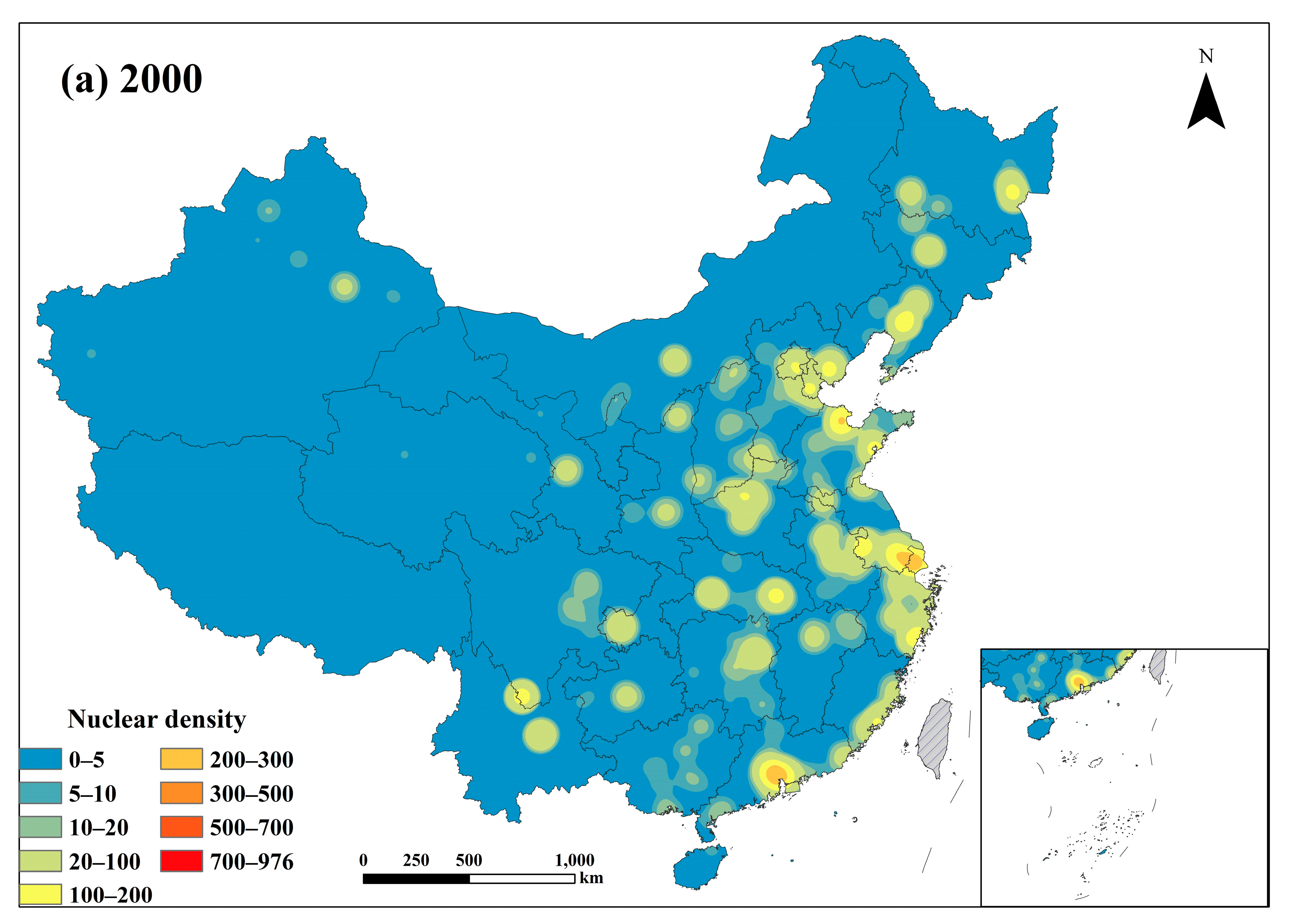
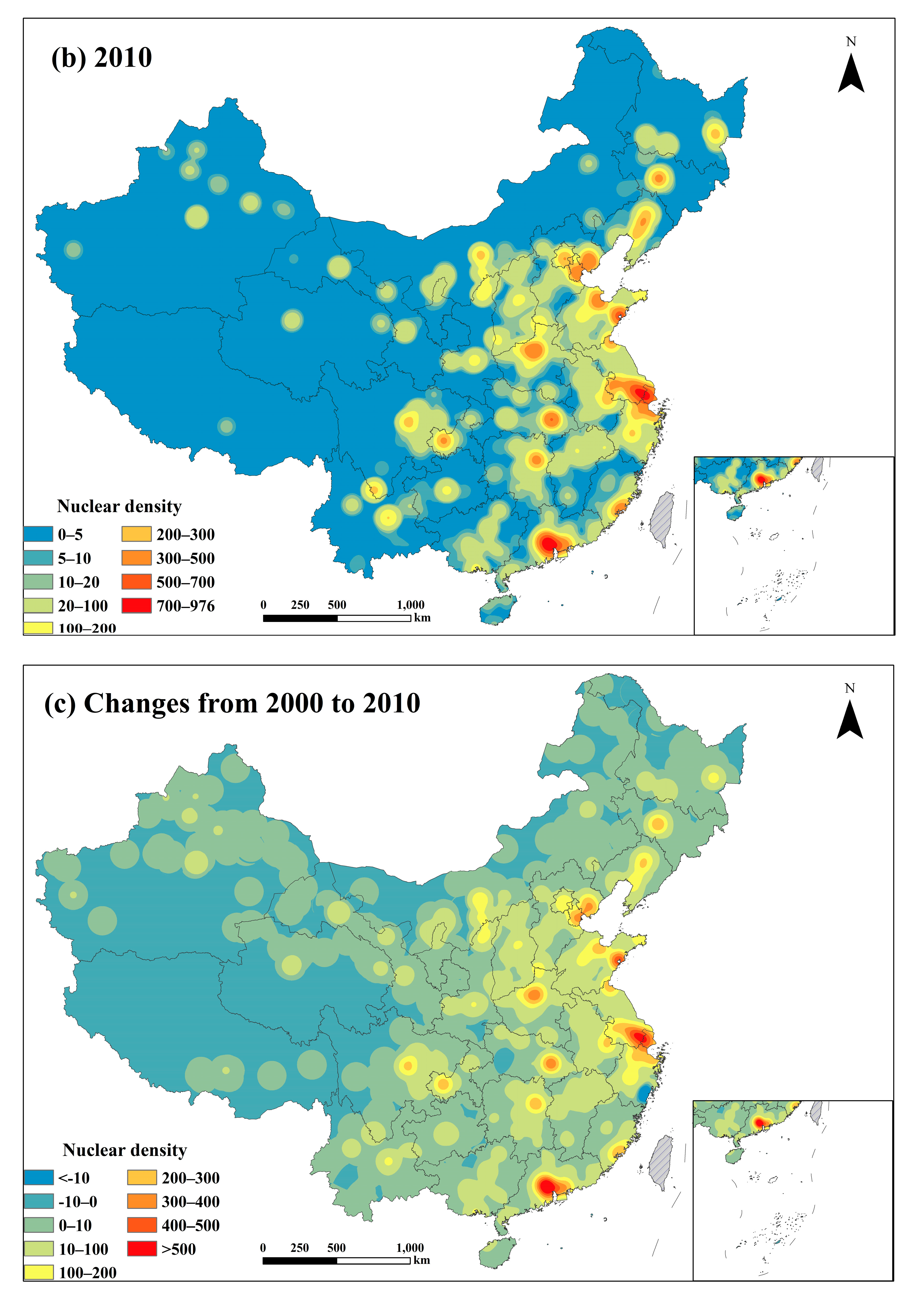
3.2. Spatialization Feature Analysis of the Current Industrial Output Value

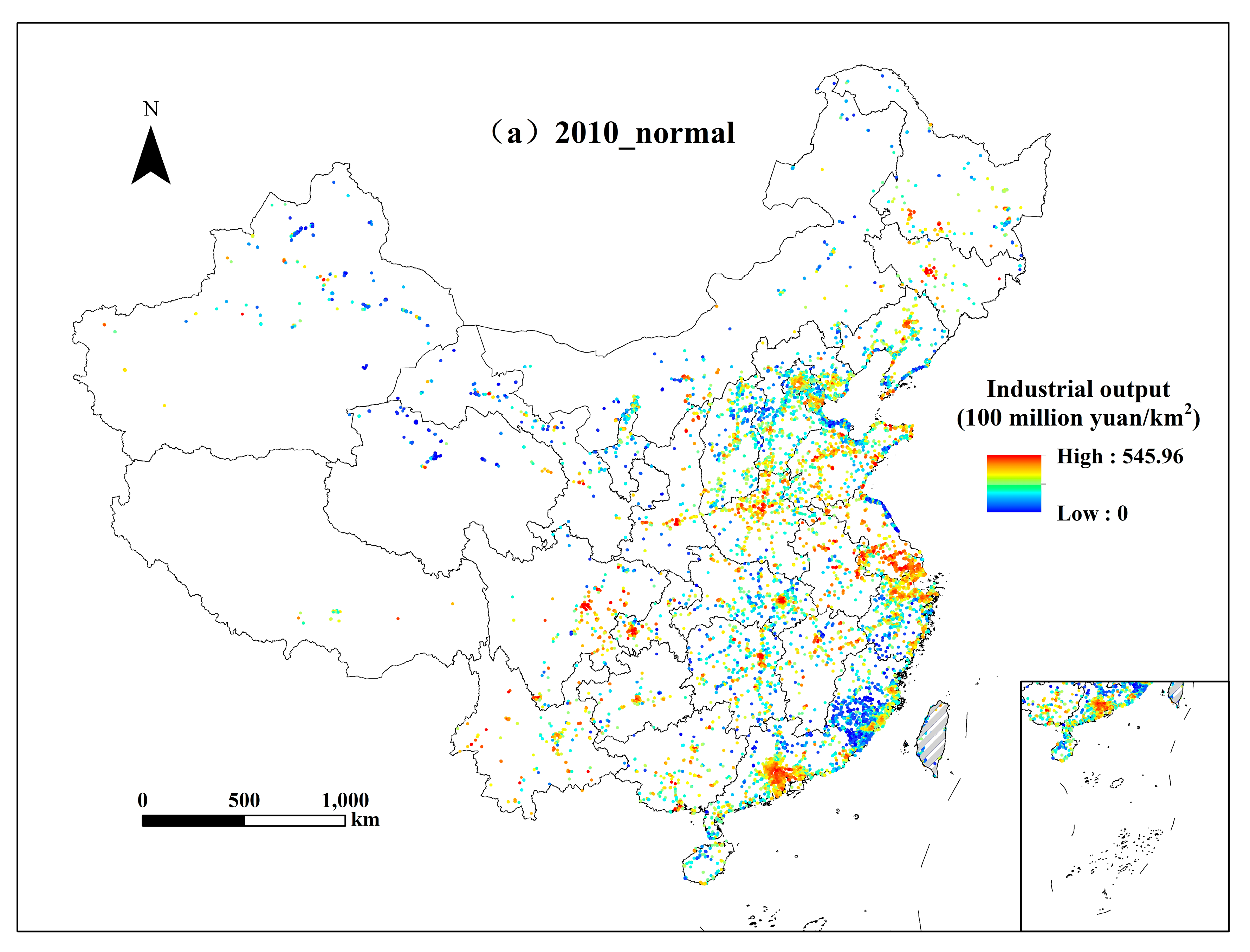
We analyzed the overall spatial distribution features of the industrial output value by kernel density estimation. In terms of bandwidth selection, after numerous attempts and based on literature studies, we selected 100 km as the bandwidth to conduct spatial kernel density analysis on China’s industrial output value from 2000 to 2010. In the selection of weights, because it is impossible to determine whether the industrial output value of each point comes from a certain industry, we do not distinguish the population field. The default is therefore ‘none’, which means the default count, that is, the weight of each point, is equal to 1 (as shown in Figure 3).

The simulation results (Figure 3) show that the kernel density of China’s industrial output value presented an increasing trend from 2000 to 2010. Especially in the Yangtze River Delta, the Pearl River Delta, and the Bohai Rim region, this trend was significant; at the same time, the kernel density values in some regions of Henan, Hubei, Hunan, Sichuan-Chongqing economic zone, Jilin, and Liaoning also increased significantly. These regions have suitable geographical conditions and abundant natural resources; because of the Yangtze River and the Bohai economic rim, transportation is highly convenient. Therefore, the industry has well developed in the past decade, and the industrial development presents an expanding trend, with the formation of several industrial parks. From 2000 to 2010, China’s industrial output value increased significantly, along with the area of industrial land. At the same time, the spatial distribution of industrial output became more concentrated, with the formation of numerous intensively distributed industrial zones. Even in northern Xinjiang, Inner Mongolia, Heilongjiang, Yunnan, Guizhou, and most regions of Guangxi, the kernel density values showed an obvious increase of 0–10/km². However, in southern Xinjiang, some regions of Tibet, and southern Qinghai, the overall output values were relatively low, and the kernel density values of some regions even showed a decreasing trend. The main reason for such a development is that these regions are located inland, with inconvenient traffic conditions and relatively poor terrain conditions, leading to a patchy industrial distribution and, consequently, slow industrial development.

3.3. Industrial Output Spatialization under Scenarios RCP4.5 and RCP8.5

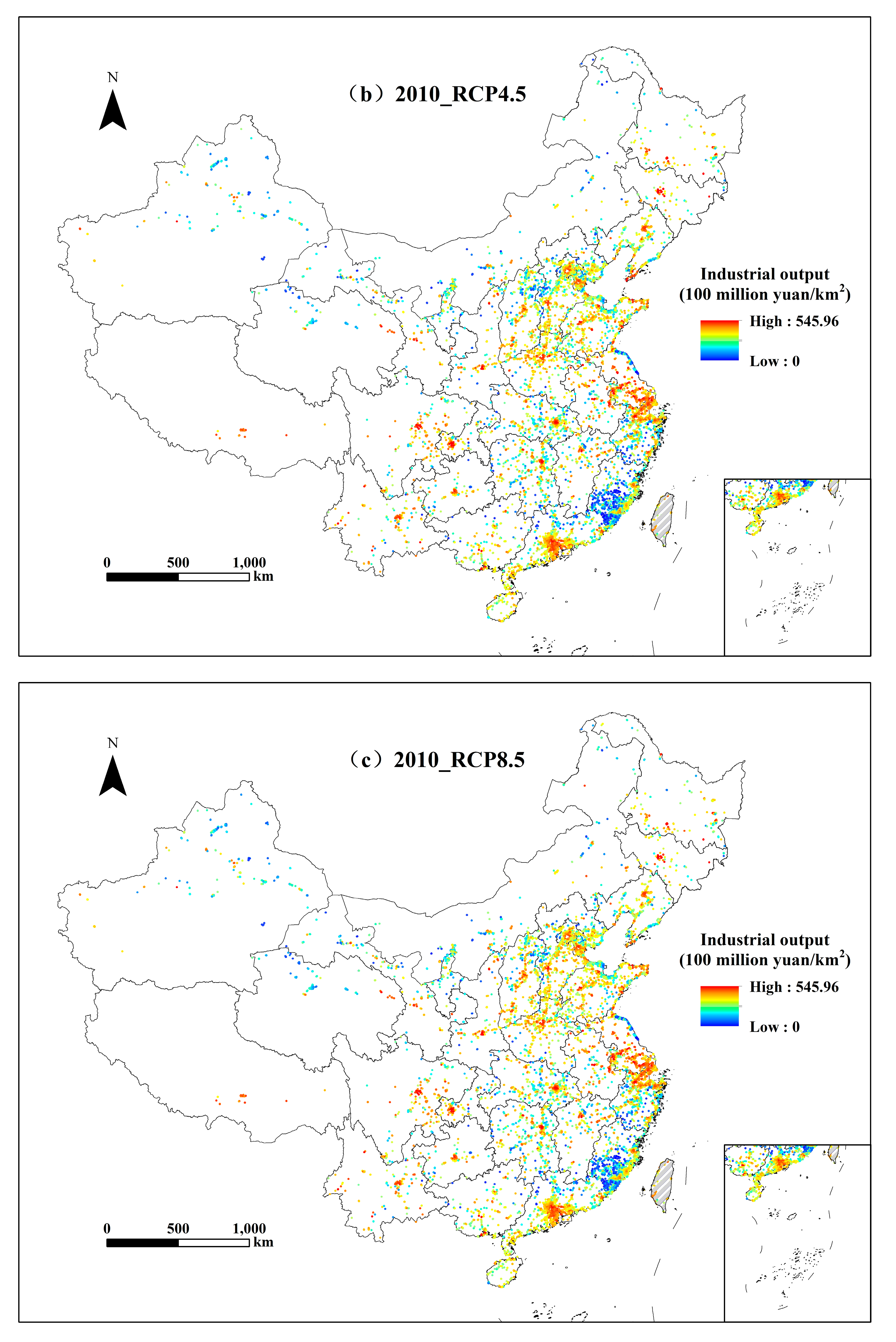
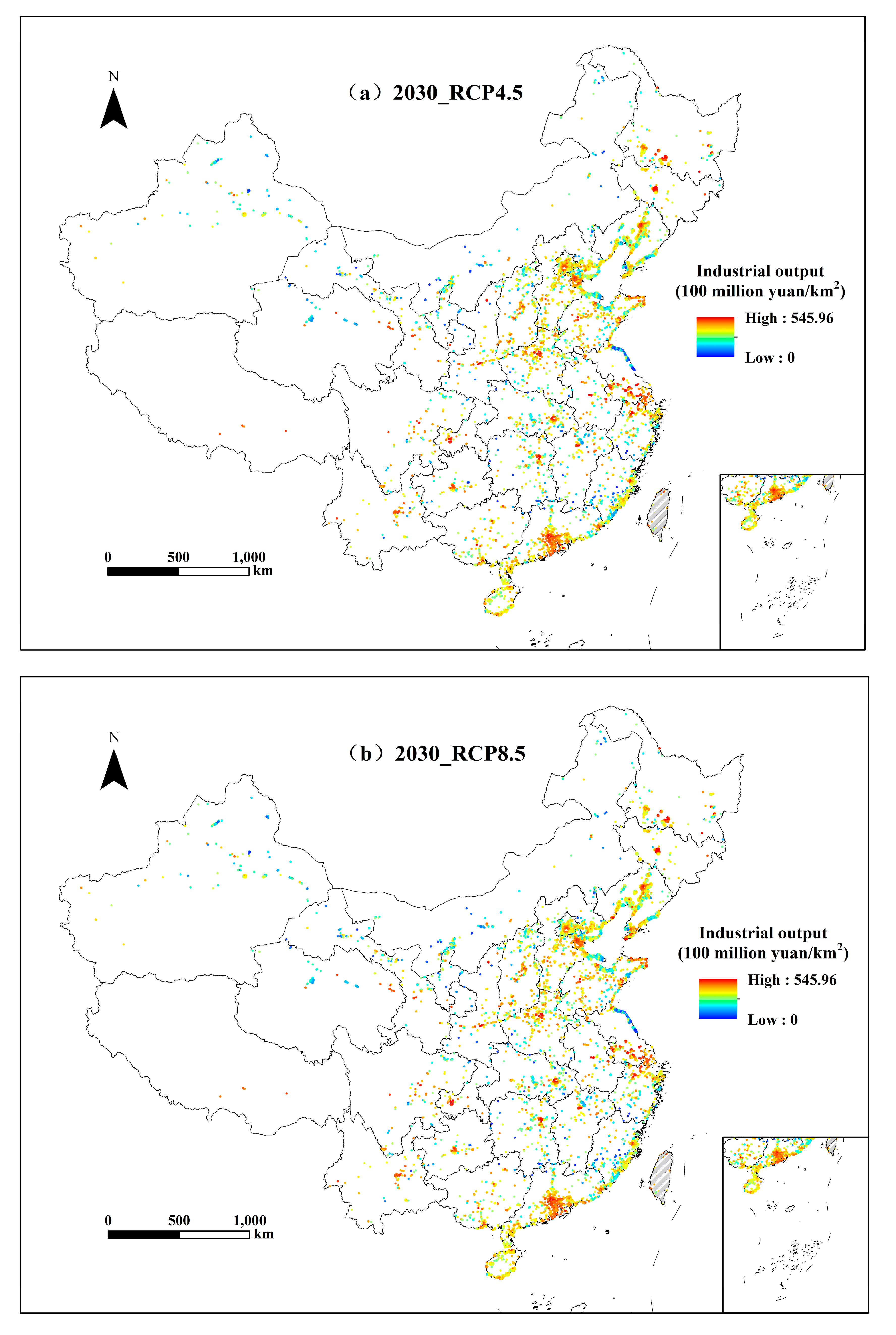
The average accuracy of the industrial output value obtained by the random forest simulation was 93.77%, which proves that the random forest model has a high simulation accuracy and can be used to study industrial output spatialization under different climate change scenarios. According to the climate factor data in China and the random forest model under different scenarios, the spatial changes of the proportions of China’s industrial output under the climate scenarios RCP4.5 and RCP8.5 from 2010 to 2050 were analyzed (Figure 4 and Figure 5).

As sown in Figure 4a–c, the proportions of the industrial output under scenarios RCP4.5 and 8.5 are lower than that of the current industrial output value; especially in the central, eastern, and southern coastal regions, the proportion of the industrial output showed a significant decrease.

According to Figure 4 and Figure 5, the proportions of the industrial output values under different climate change scenarios were different. Overall, the regions with higher proportions of the industrial output value were mainly distributed in the Bohai Rim region, the Yangtze River Delta coastal region, and the Pearl River Delta region, while the proportions of the industrial output value in the northwestern region were generally low. Under scenarios RCP4.5 and 8.5, the proportions of the industrial output value showed a declining trend from 2010 to 2050. For industrial land, from 2010 to 2050, the proportion of industrial land is predicted to show an increasing trend. In 2030, the predicted proportion of industrial land increases by 1.37 ‰ compared with 2010. In particular, industrial land in the Beijing-Tianjin-Hebei region has changed significantly, mostly characterized by an increase, whereas the middle and lower reaches of the Yangtze River will mainly show a decrease. By 2050, the proportion of industrial land will be increased by 1.22 ‰ compared with 2030. By this time, the industrial land in the Beijing-Tianjin-Hebei region will have changed significantly, showing a significant decrease, but other areas around the Bohai Bay will show an increasing trend. The middle and lower reaches of the Yangtze River will mainly show a decreasing trend, along with the Pearl River Delta.

Under scenario RCP4.5, the industrial output value of the kilometer grid shows a trend of decreasing year by year. Especially from 2030, the industrial output value grid is predicted to change greatly, and the high-value areas will be significantly reduced, especially in the central and eastern plains, with obvious changes on a yearly basis. Also, from 2030, the low value of the Bohai Rim will decrease significantly, and the distribution will tend to be far away from the central area of Beijing. The Yangtze River Delta will show a reduced area of industrial land from 2030, and the industrial output value will also show a downward trend. The high value of the Pearl River Delta will remain relatively unchanged, although the distribution range will be reduced.

Under scenario RCP8.5, the industrial output value of the kilometer grid will show a downward trend on a yearly basis, but the total industrial output value will be slightly higher than that in scenario RCP4.5; the overall change trend will be similar to that under scenario RCP4.5. From 2030, the distribution area of the Bohai Rim will decrease and will be located further away from the central area of Beijing and the coastal areas. Compared with the RCP4.5 scenario, the output value of each grid will decrease. The industrial output value of the Yangtze River Delta and the Bohai Rim will also decrease on a yearly basis while moving toward the coast; the output value of each grid will be lower than that under scenario RCP4.5.

By vertically comparing the proportions of China’s industrial output in different years (Figure 5a–d), we observed that the proportions of the industrial output under scenarios RCP4.5 and RCP8.5 showed a significant decline; especially in 2050, the proportion of the industrial output value presents a significantly decreasing overall trend when compared with that in 2010. In 2010, the proportion of the industrial output value under scenario RCP4.5 ranged between 0 and 15.148‱, and that under RCP8.5 ranged between 0 and 14.984‱. By contrast, in 2050, the proportions of the industrial output under scenarios RCP4.5 and RCP8.5 decrease by 0.352 and 0.352‱, respectively.

3.4. Annual Change Analysis of Industrial Output under Different Climate Scenarios

The greatest contribution of radiative forcing comes from the increasing CO₂ concentration in the atmosphere. Under scenario RCP4.5, radiative forcing will stabilize at 4.5 w/m² after 2100, and the CO₂ emission concentration will reach 850 mL/m³. By contrast, under scenario RCP8.5, radiative forcing will stabilize at 8.5 w/m² after 2100, and the CO₂ emission concentration will reach 1370 mL/m³. Previous studies have shown that the main cause of climatic changes is the burning of fossil fuels. In particular, CO₂ generated in industrial processes is an important cause of climate change. Under scenarios RCP4.5 and RCP8.5 (

Table 4. Industrial output values and their proportions from 2010 to 2050 under scenarios RCP4.5 and RCP8.5.

	2010		2020		2030		2050
	Total Output Value (100 million yuan)	Average Proportion (‱)	Total Output Value (100 million yuan)	Average Proportion (‱)	Total Output Value (100 million yuan)	Average Proportion (‱)	Total Output Value (100 million yuan)	Average Proportion (‱)
Normal scenario	157,902.4	0.505
RCP4.5	168,947.9	0.536	364,338.8	0.275	386,182.8	0.236	442,109.3	0.184
RCP8.5	171,140.2	0.536	344,795.1	0.278	395,037.1	0.236	456,056.6	0.184

), since the industrial output value is positively correlated with CO₂ concentration, to some extent, the total industrial output value also presents a relatively obvious increasing trend with increasing CO₂ concentrations. However, under scenarios RCP4.5 and RCP8.5, climatic changes will greatly fluctuate. From 2010 to 2050, the air temperature under scenarios RCP4.5 and RCP8.5 is predicted to increase by 1.47 and 2.19 °C, respectively, whereas precipitation is predicted to increase by 24.58 and 17.53 mm, respectively. At the same time, the frequency of extreme weather events will most likely increase. Climatic changes under different scenarios have certain impacts on the change of the industrial output value. The annual average growth rate of industrial output from 2010 to 2020 under scenarios RCP4.5 and RCP8.5 is predicted to be 7.988% and 7.256%, respectively, while the average annual growth rate of industrial output from 2030 to 2050 is predicted to decrease to 0.679% and 0.721%, respectively.

4. Conclusions and Discussion

Global climatic changes have become one of the key issues in many scientific fields. As a pillar industry of the national economy, the industry should be responsible for climatic changes, while it is also greatly affected by such changes. In this paper, taking mainland China as an example, we obtained the spatialized datasets of the current industrial output from remote sensing retrieval. By combination with the results of CMIP5 multi-mode climate coupling, we constructed the future spatialized model of industrial output values under different climate scenarios, based on the random forest method in machine learning. This model breaks the limit of administrative boundaries and can intuitively analyze the quantitative differences and the spatiotemporal distribution characteristics of industrial output on the grid scale. Our results provide data support for the classification of key industrial regions and the assessment of industrial land efficiency in China under different climate change scenarios. In particular, these results lay a foundation for the assessment of exposure degree, vulnerability, and risk of the industry against the background of climate change.

Our study shows that, under the two higher emission intensities (RCP4.5 and RCP8.5), the population is large, the science and technology innovation is sluggish, and the energy and resource use efficiency is low [36]. As a consequence, the industrial output value increases slowly. In particular, the average proportion of the industrial output value presents a sharply decreasing trend under industrial land expansion and a slow growth of industrial output, indicating the unbalanced development of the industrial output value. Based on the overall development of industrial output throughout China, the regions with higher proportions of the industrial output value are concentrated in the Bohai Rim region, the Yangtze River Delta coastal region, and the Pearl River Delta region, where the land area is small and the population and resources are highly concentrated. However, in the northwestern regions, with a large land area and a sparse population, the proportion of the industrial output value is generally low. In combination with regional development plans, these findings lay a solid foundation for the future adjustment and optimization of industrial layout and structure, strictly controlling the implementation of projects with high pollution and high energy consumption and promoting the development of clean-energy industries and new technological and low-carbon industries.

Exposure of the vulnerability of the industrial economic system, through risk assessment and cost-benefit analysis, is an effective way to further reveal the impacts of climate change on the economic development of industrial production, a pillar industry in China. At the same time, with binding greenhouse gas emission reduction obligations, actively adjusting the industrial economic structure and industrial layout, strictly controlling the implementation of high-pollution and high-energy-consuming projects, and actively promoting the development of clean energy industries can effectively guarantee the improvement of the industrial economy.

Our study has some limitations, however, which require further work:

Land use data are emphasized in this article. In the spatialization of industrial output value, all industrial output values were generated for industrial land. Industrial land data are generally current or past industrial land monitoring data, mostly generated by land use simulation methods. However, CMIP5 has achieved 2100 in different climate change scenarios. If the future industrial land in this model is replaced with the updated, predicted industrial land monitoring data, the spatial accuracy of industrial output value will be improved.

Although we selected numerous influencing factors for the spatial analysis of the industrial output value, more factors exist, such as policy influence, fixed asset input, and laborer health degree. However, because of the lack of such data, these factors are not considered here. At the same time, in the spatialized model of industrial output value under different climate scenarios, the possibility of changes in the influencing factors is considered; for example, changes in the elevation may affect plant site selection, but it is difficult to obtain such data, especially in the context of future changes. However, we stress that this paper focuses on the effects of climate change, and therefore, other indicators are assumed to remain unchanged. In the future, relevant uncertainty research should, however, be considered.

References

1. Hewison, D.; Kuras, M. Book reviews. J. Anal. Psychol. 2005, 50, 395–403. [Google Scholar] [CrossRef]
2. Ahn, S.E.; Steiguer, J.E.D.; Palmquist, R.B.; Holmes, T.P. Economic Analysis of the Potential Impact of Climate Change on Recreational Trout Fishing in the Southern Appalachian Mountains: An Application of a Nested Multinomial Logit Model. Clim. Chang. 2000, 45, 493–509. [Google Scholar] [CrossRef]
3. Salgotra, R.K.; Zargar, S.M.; Sharma, M.; Sood, M. Traditional Knowledge: A Therapeutic Potential in the Scenario of Climate Change for Sustainable Development. Development 2018, 61, 140–148. [Google Scholar] [CrossRef]
4. Jajer, J. Climate and Energy System; China Meteorological Press: Beijing, China, 1988. (In Chinese) [Google Scholar]
5. Thornes, J.E. The impact of weather and climate on transport in the UK. Prog. Phys. Geogr. Earth Environ. 1992, 16, 187–208. [Google Scholar] [CrossRef]
6. Mall, R.K.; Singh, R.; Gupta, A.; Srinivasan, G.; Rathore, L.S. Impact of Climate Change on Indian Agriculture: A Review. Clim. Chang. 2007, 82, 225–231. [Google Scholar] [CrossRef] [Green Version]
7. Song, W.; Pijanowski, B.C. The effects of China’s cultivated land balance program on potential land productivity at a national scale. Appl. Geogr. 2014, 46, 158–170. [Google Scholar] [CrossRef]
8. Lehr, U.; Nieters, A.; Drosdowski, T. Extreme Weather Events and the German Economy: The Potential for Climate Change Adaptation; Springer International Publishing: Basel, Switzerland, 2016. [Google Scholar]
9. Marshall, N.A.; Tobin, R.C.; Marshall, P.A.; Gooch, M.; Hobday, A.J. Social Vulnerability of Marine Resource Users to Extreme Weather Events. Ecosystems 2013, 16, 797–809. [Google Scholar] [CrossRef]
10. Linnenluecke, M.K.; Griffiths, A.; Winn, M. Extreme Weather Events and the Critical Importance of Anticipatory Adaptation and Organizational Resilience in Responding to Impacts. Bus. Strategy Environ. 2012, 21, 17–32. [Google Scholar] [CrossRef]
11. Wedawatta, G.; Ingirige, B. A conceptual framework for understanding resilience of construction SMEs to extreme weather events. Built Environ. Proj. Asset Manag. 2016, 6, 428–443. [Google Scholar] [CrossRef]
12. Kumar, A.; Tripathi, P.; Singh, K.K.; Mishra, A.N. Impact of climate change on agriculture in eastern Uttar Pradesh and Bihar states (India). Mausam 2011, 62, 171–178. [Google Scholar]
13. Muoz-Rojas, M.; Abd-Elmabod, S.K.; Zavala, L.M.; Rosa, D.D.L.; Jordán, A. Climate change impacts on soil organic carbon stocks of Mediterranean agricultural areas: A case study in Northern Egypt. Agric. Ecosyst. Environ. 2017, 238, 142–152. [Google Scholar] [CrossRef]
14. Awoye, O.H.R.; Pollinger, F.; Agbossou, E.K.; Paeth, H. Dynamical-statistical projections of the climate change impact on agricultural production in Benin by means of a cross-validated linear model combined with Bayesian statistics. Agric. For. Meteorol. 2017, 234–235, 80–94. [Google Scholar] [CrossRef]
15. Gigantesco, A.; Giuliani, M. Quality of life in mental health services with a focus on psychiatric rehabilitation practice. Annali dell’Istituto Superiore di Sanita 2011, 47, 363. [Google Scholar]
16. Song, W.; Deng, X. Land-use/land-cover change and ecosystem service provision in China. Sci. Total Environ. 2017, 576, 705–719. [Google Scholar] [CrossRef]
17. Li, S.; He, F.; Zhang, X.; Zhou, T. Evaluation of global historical land use scenarios based on regional datasets on the Qinghai-Tibet Area. Sci. Total Environ. 2019, 657, 1615–1628. [Google Scholar] [CrossRef]
18. Zhang, X.; Zhang, Y.; Liu, L.; Zhang, J. Zoning by land types based on SOFM network:A case study on transect of eastern Tibetan Plateau. Geogr. Res. 2013, 32, 839–847. [Google Scholar]
19. Min, Z.; Weiming, C.; Chenghu, Z.; Manchun, L.; Nan, W.; Qiangyi, L. GDP Spatialization and Economic Differences in South China Based on NPP-VIIRS Nighttime Light Imagery. Remote Sens. 2017, 9, 673. [Google Scholar]
20. Tobler, W.R. Smooth pycnophylactic interpolation for geographical regions. Publ. Am. Stat. Assoc. 1979, 74, 519–530. [Google Scholar] [CrossRef]
21. Rase, W.D. Volume-preserving interpolation of a smooth surface from polygon-related data. J. Geogr. Syst. 2001, 3, 199–213. [Google Scholar] [CrossRef]
22. Li, L.; Li, J.; Jiang, Z.; Zhao, L.; Zhao, P. Methods of Population Spatialization Based on the Classification Information of Buildings from China’s First National Geoinformation Survey in Urban Area: A Case Study of Wuchang District, Wuhan City, China. Sensors 2018, 18, 2558. [Google Scholar] [CrossRef] [Green Version]
23. Du, G.; Zhang, S. Spatializing population data of jilin province. In Proceedings of the 2011 International Conference on Remote Sensing, Environment and Transportation Engineering, Nanjing, China, 24–26 June 2011. [Google Scholar]
24. Wang, L.; Wang, S.; Zhou, Y.; Liu, W.; Hou, Y.; Zhu, J.; Wang, F. Mapping population density in China between 1990 and 2010 using remote sensing. Remote Sens. Environ. 2018, 210, 269–281. [Google Scholar] [CrossRef]
25. Li, X.; Yeh, G.O. Analyzing spatial restructuring of land use patterns in a fast growing region using remote sensing and GIS. Landsc. Urban Plan. 2004, 69, 335–354. [Google Scholar] [CrossRef]
26. Doulamis, N.; Voulodimos, A.; Preka, D.; Ioannidis, C.; Fritsch, D. An efficient framework for spatiotemporal 4D monitoring and management of real property. In Proceedings of the High-Level Joint FIG/World Bank Conference on Sustainable Real Estate Markets—Policy Framework and Necessary Reforms, Athens, Greece, 19 September 2016. [Google Scholar]
27. Taylor, K.E.; Stouffer, R.J.; Meehl, G.A. An Overview of CMIP5 and the Experiment Design. Bull. Am. Meteorol. Soc. 2012, 93, 485–498. [Google Scholar] [CrossRef] [Green Version]
28. Sillmann, J.; Kharin, V.V.; Zhang, X.; Zwiers, F.W.; Bronaugh, D. Climate extremes indices in the CMIP5 multimodel ensemble: Part 1. Model evaluation in the present climate. J. Geophys. Res. Atmos. 2013, 118, 1716–1733. [Google Scholar] [CrossRef]
29. Ongoma, V.; Chen, H.; Gao, C.; Nyongesa, A.M.; Polong, F. Future changes in climate extremes over Equatorial East Africa based on CMIP5 multimodel ensemble. Nat. Hazards 2018, 90, 901–920. [Google Scholar] [CrossRef]
30. Qian, X.; Song, W.; Zhu, H. A 1-km grid dataset of industrial output value in China (2010). China Sci. Data 2018, 3, 1–13. [Google Scholar]
31. Gramacki, A. Nonparametric Kernel Density Estimation and Its Computational Aspects; Springer International Publishing: Berlin, Germany, 2018; pp. 25–62. [Google Scholar] [CrossRef]
32. Qahtan, A.; Wang, S.; Zhang, X. KDE-Track: An Efficient Dynamic Density Estimator for Data Streams. IEEE Trans. Knowl. Data Eng. 2017, 29, 642–655. [Google Scholar] [CrossRef] [Green Version]
33. Liu, J.; Zhang, Z.; Xu, X.; Kuang, W.; Zhou, W.; Zhang, S.; Li, R.; Yan, C.; Yu, D.; Wu, S.; et al. Spatial patterns and driving forces of land use change in China during the early 21st century. J. Geogr. Sci. 2010, 20, 483–494. [Google Scholar] [CrossRef]
34. Sui, Y.; Lang, X.; Jiang, D. Time of emergence of climate signals over China under the RCP4.5 scenario. Clim. Chang. 2014, 125, 265–276. [Google Scholar] [CrossRef]
35. Thomson, A.M.; Calvin, K.V.; Smith, S.J.; Kyle, G.P.; Volke, A.; Patel, P.; Delgado-Arias, S.; Bond-Lamberty, B.; Wise, M.A.; Clarke, L.E. RCP4.5: A pathway for stabilization of radiative forcing by 2100. Clim. Chang. 2011, 109, 77. [Google Scholar] [CrossRef] [Green Version]
36. Meinshausen, M.; Smith, S.J.; Calvin, K.; Daniel, J.S.; Kainuma, M.L.T.; Lamarque, J.F.; Matsumoto, K.; Montzka, S.A.; Raper, S.C.B.; Riahi, K.; et al. The RCP greenhouse gas concentrations and their extensions from 1765 to 2300. Clim. Chang. 2011, 109, 213. [Google Scholar] [CrossRef] [Green Version]
Figure 1. Geographic map of China.
Ijgi 09 00724 g001
Figure 2. Schematic presentation of the research design.
Ijgi 09 00724 g002
Figure 3. Kernel density estimation values of industrial output in 2000 (a) and 2010 (b); variation of kernel density estimation values of industrial output from 2000 to 2010 (c).
Ijgi 09 00724 g003aIjgi 09 00724 g003b
Figure 4. Spatial distribution diagrams of the proportions of China’s industrial output in 2010 under the scenarios of normal condition (a), RCP4.5 (b), and RCP8.5 (c).
Ijgi 09 00724 g004aIjgi 09 00724 g004b
Figure 5. Spatial distribution diagrams of the proportions of China’s industrial output from 2030 to 2050 under scenarios RCP4.5 ((a) for 2030_RCP4.5 and (c) for 2050_RCP4.5) and RCP8.5 ((b) for 2030_RCP8.5 and (d) for 2050_RCP8.5).
Ijgi 09 00724 g005aIjgi 09 00724 g005b