Eutrophication Monitoring for Lake Pamvotis, Greece, Using Sentinel-2 Data

Abstract

The use of remote sensing to monitor inland waters and their current state is of high importance, as fresh waters are the habitat of many species of flora and fauna, and are also important for anthropogenic activities. Water quality can be monitored by many parameters, including dissolved suspended matter, phytoplankton, turbidity, and dissolved organic matter, while the concentration of chlorophyll-a (chl-a) is a representative indicator for detecting phytoplankton and monitoring water quality. The detection of phytoplankton in water layers, through chl-a indicators, is an effective method for displaying eutrophication. Numerous scientific publications and studies have shown that remote sensing data and techniques are capable of monitoring the temporal and spatial distribution and variation of this phenomenon. This study aimed to investigate the eutrophication in Pamvotis Lake, in Ioannina, Greece with the application of chl-a detection algorithms, by using Sentinel-2 satellite imagery data for the time period of 2016–2018. The maximum chlorophyll index (MCI) and maximum peak-height (MPH) algorithms have been applied to top of atmosphere (TOA) reflectance data, to detect chl-a and monitor the trophic range of the water body. Both algorithms were correlated and resulted in Pearson’s r values up to 0.95. Finally, the chl-a concentration was estimated by applying an empirical equation that correlates the MPH and chl-a concentration developed within previous studies. Those results were further analyzed and interpreted with spatial statistical methods, to understand the spatial distribution pattern of the eutrophication in our study area. Our results demonstrated that Pamvotis Lake is a eutrophic lake, and the highest chl-a concentration was located in the east and south-east of the lake during the study period. Sentinel-2 data can be a useful tool for lake managers, in order to estimate the spatial distribution of the chl-a concentration and identify areas prone to eutrophication, as well as the coastal zones that may influence the lake through water canals.

1. Introduction

Water is a valuable natural element that covers 70% of our planet and is essential for the flourishing of all forms of life. Water can be found in fresh water bodies, such as lakes, rivers, and groundwater, as well coastal water bodies and oceans [1]. Water is also important for human activities and the production of commodities. Inland waters are the habitat of several species of flora and fauna. With the increase in human activities (urban development, industries, growth of population, and agriculture) the quality of water bodies has been dramatically affected, and this has lead to many negative impacts on their current state [2].

Eutrophication is the phenomenon where the minerals and nutrients increase in a body of water and, as a result, algae and aquatic plant life increase. A major cause for the increase of phytoplankton is the water pollution and contamination. The organic wastes, detergents, and fertilizers that end up in reservoirs produce nutrients due to the nitrogen (N), phosphorus (P), and potassium (K) they contain, and thus become food for phytoplankton [3]. The development of phytoplankton communities in the aquatic body due to the consumption of the available oxygen also leads to an increase in the water turbidity. The production of a green layer on the top of water reduces the productivity of fishing activities and also provides an inhospitable environment for other forms of life [4].

The quality of inland waters has been a crucial environmental issue in recent years and many studies have focused on analyzing and predicting the phenomenon of eutrophication so as to give possible causes and possible solutions for the problem. Remote sensing plays a vital role in monitoring and understanding of the composition of eutrophication, as well as the status of the water. Chlorophyll and other pigments absorb and reflect light at certain regions of the electromagnetic spectrum—absorbing in the blue and red regions of visible spectrum and reflecting in the green [5]. As a result, remote sensing data of high spatial and high temporal resolution can help to monitor chlorophyll-a (chl-a) distribution and concentration in inland water bodies.

In various studies and scientific research, chl-a algorithms have been built and designed to identify and derive the chl-a concentration. The related literature has a variety of studies focusing on monitoring chl-a as an indicator of water quality with remote sensing data and techniques based on inland waters (mostly lakes). Kravitz et al. [6] performed a study over small inland waters to retrieve chl-a from Sentinel-3 ocean and land color instrument (OLCI) data. The Sentinel-3 was also used among with the Sentinel-2 Multispectral Imager (MSI) in order to compare the retrieved chl-a in two large Italian lakes [7].

The Sentinel-2 MSI is an earth observation mission by the Copernicus program with two polar-orbiting satellites placed in the same sun-synchronous orbit (Sentinel-2A and Sentinel-2B). These sensors have a variety of quality characteristics, such as high resolution and multi-spectral imaging, and are designed to give a high revisit frequency of 2–3 days. The Sentinel-2 carries an optical instrument with 13 spectral bands: four bands at 10 m spatial resolution, six bands at 20 m, and three bands at 60 m.

The Sentinel-2 MSI is one of the sensors that has been used in recent years to provide data and monitoring of the physical states of marine, ocean, and coastal ecosystems. Some studies have focused on water quality estimation in inland waters and whether the land use is an important parameter for water pollution and contamination while others emphasize the spectral response [8,9,10,11,12,13]. Furthermore, the Sentinel-2 MSI has been compared with the Landsat-8 operational land imager (OLI) and it was observed that during pre-monsoon and post-monsoon seasons, the chl-a from the MSI is over estimated compared to the OLI [14].

Some indices were also developed based on the spectral difference between the clear and the eutrophic water. The maximum chlorophyll index (MCI) has been developed to measure the height of the peak in water, with a reflectance at 709 nm, relative to a baseline between 681 nm and 753 nm for medium resolution imaging spectrometer (MERIS) bands [15]. Through several studies, it has emerged that the width of the peak close to 705 nm is associated with high levels of chl-a [16]. The MCI algorithm was characterized specifically for the MERIS toolbox; therefore, the fluorescence line height (FLH)/MCI processor in Sentinel Application Platform (SNAP) contains an additional factor (k = 1.005) to correct for the influence of thin clouds [17].

Most studies in this area have focused on retrieving the chl-a concentration. The Sentinel-2 MSI has been extensively used for monitoring and observing cyanobacteria bloom events in eutrophic lakes. In [18], the authors analyzed and tested the chl-a indicators and empirical equations for chl-a concentration retrieval to derive the best-performing results through testing the top of atmosphere (TOA) and bottom of atmosphere (BOA) reflectance. According to this research, the best root mean square (RMS) error for the TOA data was achieved with a modified algorithm, named Maximum Peak-Height (MPH) [19], with RMS = 18 μg/L and R² = 0.72, and with similarity to the FLH [20].

The MPH algorithm searches for the position and magnitude of the maximum peak in the Red/NIR at 681 nm, 709 nm, and 753 nm and uses a baseline between 664 nm and 885 nm for MERIS bands. The algorithm is designed to retrieve the concentration of chl-a through an empirical equation. Even if both the MCI and MPH algorithms have been developed for MERIS bands, they can be reformed based on Sentinels-2 bands: B4, B5, B6, and B8A, with 665 nm, 705 nm, 740 nm, and 865 nm central wavelengths, respectively. Thus both algorithms have been applied in Sentinel-2, in various areas of study [18,21,22].

This paper aims to explore the MCI and MPH products based on Sentinel-2 data in the shallow lake, Pamvotis, Greece, with extremely high biomass, floating algae, and aquatic vegetation. Furthermore, we estimate the spatial chl-a concentration for a three year period based on an empirical equation, developed within previous research for another similar study area. The spatial-temporal dataset developed was further statistically analyzed in order to understand the spatial distribution patterns of chl-a and to highlight the usability of the MPH algorithm for the detection of phytoplankton and aquatic vegetation. Even if various studies have been conducted for Pamvotis lake, these were focused mainly on water quality estimation based on point field measurements, short range forecasting, and identification of the contributing environmental parameters associated with eutrophication in this lake, while their analysis lacks, to the best of our knowledge, any spatial-temporal context [23,24,25,26,27,28,29].

2. Materials and Methods

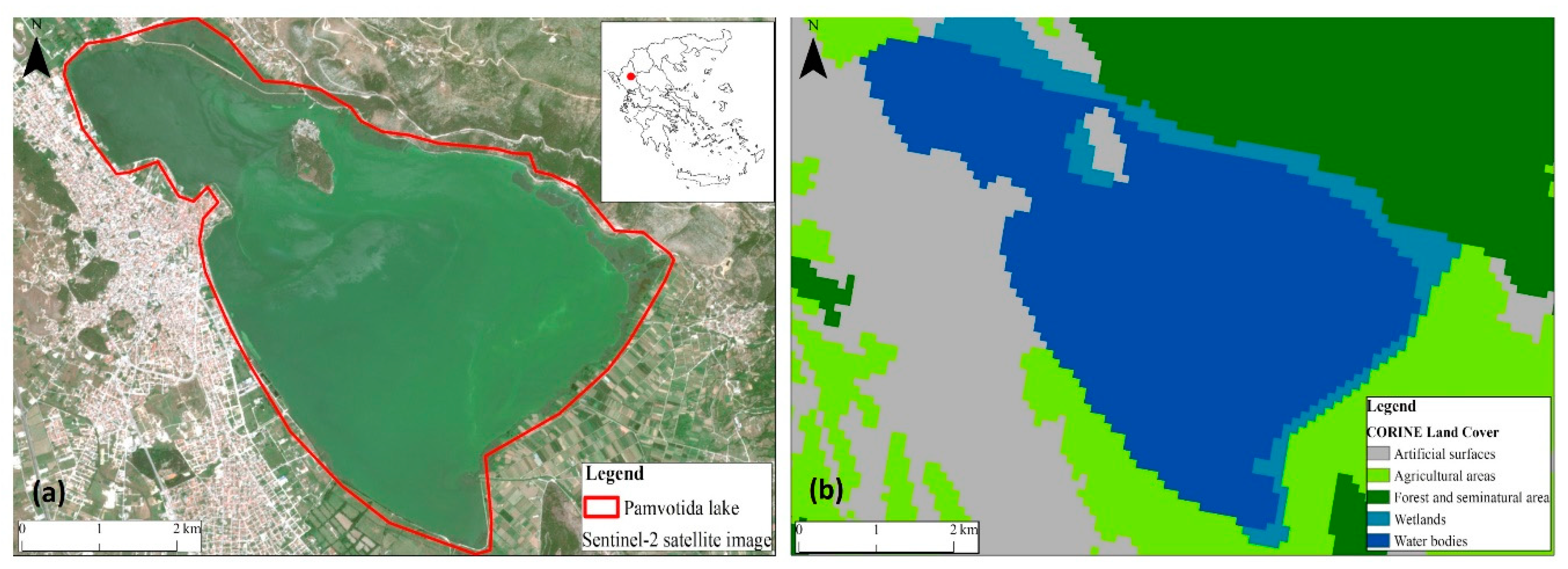
2.1. Study Area and Data

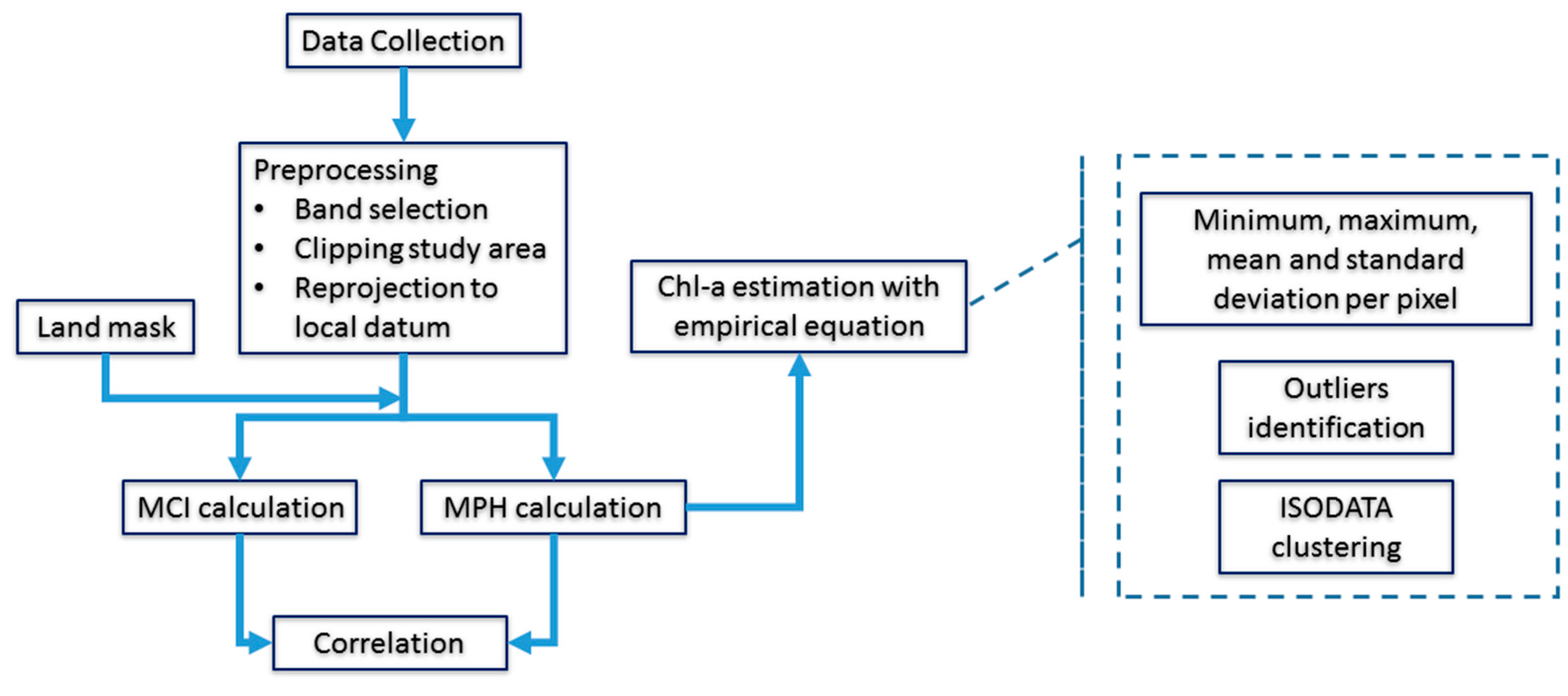
The lake of Pamvotis, also known as Lake of Ioannina (Figure 1a), is located in the regional unit of Ioannina in northern Greece. The lake is situated at an altitude of 470 m above sea level and has a total area of 24 km², length of 7.5 km, and width from 1 to 5 km. A small island is located close to the north-west coast, including a traditional settlement of historic importance, while the city of Ioannina is located on the lake’s western shore. Pamvotis has a remarkable endemic ecosystem with a variety of imported and native species [30]. However, urban growth leads to landscape fragmentation and, consequently, the lake has suffered many changes in ecological composition, as well as disruption of its hydrological cycle. The city’s population has increased and thus so have their needs; so, as a result, the production of commodities has increased, meaning an increase in agricultural and industrial activities. These production activities have lead to an increase of wastes that are channeled into Pamvotis [31].

The configuration of land-cover types (Figure 1b) reveals the human activities and the effects of the lake’s environment and degradation. The lake is mainly covered by urban and agricultural land. Organic wastes and fertilizers from the urban area and land crops eventually arrive in the lake, causing crucial environmental issues. However, the degradation of the lake’s landscape has become apparent in recent years, with the increase of aquatic plants, turbidity, unpleasant odors, and short-term fishing bans to protect the fish stocks in the lake basin.

In order to explore the quality of the lake’s water, 65 cloud-free satellite images were retrieved in JPEG 2000 format, acquired by the Sentinel-2A and Sentinel-2B MSI satellites. The dataset consist of the years 2016–2018 (15, 21, and 29 for the years 2016, 2017, and 2018, respectively) and the product type is Level-1C. Level-1C products are radiometrically corrected, providing the top of atmosphere (TOA) reflectance and geometrically corrected using a 90 m digital elevation model (DEM) (PlanetDEM 90) by shuttle radar topography mission (SRTM) v4.1 in UTM (Universal Transverse Mercator)/WGS84.

2.2. Methodology

For land masking, a number of indices were tested. In particular, the normalized difference moisture index (NDMI), automated water extraction index (AWEI), water ratio index (WRI), normalized difference water index (NDWI), and modification of normalized difference water index (MNDWI) were applied in the study area to separate the land from the water. The NDWI provided the best results in order to create a mask for the land area. During the pre-processing stage, a land mask was developed to separate the land from the lake based on NDWI, as follows [32]:

$$\mathrm{NDWI}=\frac{\mathrm{G}-\mathrm{NIR}}{\mathrm{G}+\mathrm{NIR}}$$

(1)

where G is the green band and NIR is the near infrared. The index is based on the difference where the reflectance of the water features are higher in the visibly green and lower in the near infrared zone of the electromagnetic spectral information. The values of the NDWI range from −1 to +1, where positive values correspond to water areas and negative values to soil, vegetation, and urban landscape characteristics [32]. The land mask was performed on a cloud free satellite image of 13/08/2018.

To monitor the eutrophication, we applied two detection algorithms, the MCI and the MPH. The MCI was originally developed for MERIS sensor data with the purpose to produce daily data for tracking, detecting, and mapping phytoplankton and aquatic vegetation [15]. The MCI measures the height of its peak reflectance at 705 nm of the electromagnetic spectrum, while it is used as a baseline for the range between 665 nm and 740 nm regions for Sentinel-2 bands. The width of the peak near 705 nm is associated with high levels of chl-a in oceans, coastal, and terrestrial waters, as has emerged through surveys and studies. However, there are numerous of false alarms when interpreting MCI data; high values of the index in shallow waters often referred to benthic vegetation and not to algal blooms [16]. Optimization of the MCI algorithm has been achieved by including a factor, so that its efficiency is not affected by thin clouds, as discovered in recent research [17]. The MCI applied to Sentinel-2 data is described by the following equation (Equation (2)):

$$\mathrm{MCI}=\mathrm{B}5-1.005\left[\mathrm{B}4+\frac{\left(\mathrm{B}6-\mathrm{B}4\right)\left({\mathsf{\lambda }}_{\mathrm{B}5}-{\mathsf{\lambda }}_{\mathrm{B}4}\right)}{{\mathsf{\lambda }}_{\mathrm{B}6}-{\mathsf{\lambda }}_{\mathrm{B}4}}\right]$$

(2)

where B4, B5, and B6 are the reflectance and λ_B4 = 0.665 nm, λ_B5 = 0.705 nm and λ_B6 = 0.740 nm are the central wavelengths of the corresponding bands of Sentinel-2. The second algorithm to detect chl-a is the MPH, a modification of the MCI and is based on a baseline that sets the range to which we will find the position and the size of peak reflectance. The line used as a base is the length of wavelength at 665 nm and 865 nm. The wavelength at 705 nm of the electromagnetic spectrum for Sentinel-2 bands is defined as the peak point of reflectance in eutrophic waters (Figure 2) and is the active point of chl-a [18]. The MPH is designed to provide the trophic status determination and to handle three types of waters: (1) mixed oligotrophic/mesotrophic waters with low to medium biomass; (2) high biomass in eutrophic/hypertrophic waters; and (3) extreme high biomass with surface suspended algae or aquatic vegetation [19]. The MPH applied for the Sentinel-2 data is calculated as follows (Equation (3)):

$$\mathrm{MPH}=\mathrm{B}5-\mathrm{B}4-\frac{\left(\mathrm{B}8\mathrm{A}-\mathrm{B}4\right)\left({\mathsf{\lambda }}_{\mathrm{B}5}-{\mathsf{\lambda }}_{\mathrm{B}4}\right)}{{\mathsf{\lambda }}_{\mathrm{B}8\mathrm{A}}-{\mathsf{\lambda }}_{\mathrm{B}4}}$$

(3)

where B4, B5, and B8A are the reflectance and λ_B4 = 0.665 nm, λ_B5 = 0.705 nm, and λ_B8A = 0.865 nm are the central wavelengths of the corresponding bands of Sentinel-2.

The first step in our workflow was to correlate the two algorithms, MCI and MPH, and identify whether there is a strong correlation between them or not, in order to use only one of them for our further analysis. The evaluations were performed by estimating Pearson’s r correlation coefficient in order to measure the strength of the association between the MPH and MCI values for all 65 time-periods of the study (year 2016: 15 images, year 2017: 21 images, year 2018: 29 images).

During the next stage we tried to retrieve the concentration of chl-a by using models from the literature that have been developed for another study area based on in situ measurements and satellite data [18]. The chosen empirical equation correlates the MPH and the chl-a concentration for the Sentinel -2 Level-1C data. The equation applied has not been validated in our study area; however, it has been developed based on in situ measurements on four lakes in Lithuania with various characteristics, of which two are eutrophic blooming lakes with agriculture and urban land cover types in their basin. The results present much of the chl-a concentration variation and distribution and had the best RMS error, equal to 18 μg/L. The empirical equation developed for cyanobacteria rich waters is the following [18,19]:

$$\mathrm{Chla}=2223.18\ast \mathrm{MPH}+24.03.$$

(4)

In addition to analyzing the spatial distribution and aggregation of chl-a, we performed a descriptive statistical analysis. For each pixel of our study area, the minimum, maximum, mean, and standard deviation of chl-a concentration for the study period was calculated and mapped in order to identify possible causes and conditions. In statistical analysis, an important step in analyzing a variable is finding and treating the outliers, and also determining how the patterns are spatially and quantitatively distributed. Often the extreme values are present as deviations and appear in locations where they are not expected according to the variable distribution pattern [33]. For finding, treating, and interpreting the outliers, the interquartile range (IQR) method was used. The IQR approach of identifying extreme cases in datasets, uses the difference between the third and the first quartile of the data (Q3-Q1). The first quartile (Q1) is the value of the data with 25% of the values below it. The third quartile (Q3) is the value of the data with 25% of the values above it. A common rule for implementation of this method assumes that the exclusions are 1.5*IQR below Q1 or 1.5*IQR above Q3 [34]. In our study we identified only the pixels with extreme high values according to:

$$\mathrm{Outliers}={\mathrm{Q}}_3+1.5\ast \mathrm{IQR}.$$

(5)

The next step of our process was the clustering of the 65 chl-a concentrations datasets. Clustering is the process by which the pixels are grouped into a class correlated to display similar characteristics that are different from those of the other classes. In this paper we applied the Iterative Self-Organizing Data analysis technique (ISODATA), which is an unsupervised classification approach that requires the number of desired clusters, the maximum iterations, and the minimum number of pixels per cluster [35,36,37]. In order to find the optimal number of clusters, we applied a number of the most widely used methods included in the NbClust R package [38], and we finally applied the number of clusters with the highest frequency among all indices.

The above procedures were automated within the ArcGIS software v. 10.2.2, by developing graphical models and python scripts, so that anyone can reproduce the products for any study area and for any time period. Figure 3 presents the workflow of our methodology.

3. Results and Discussion

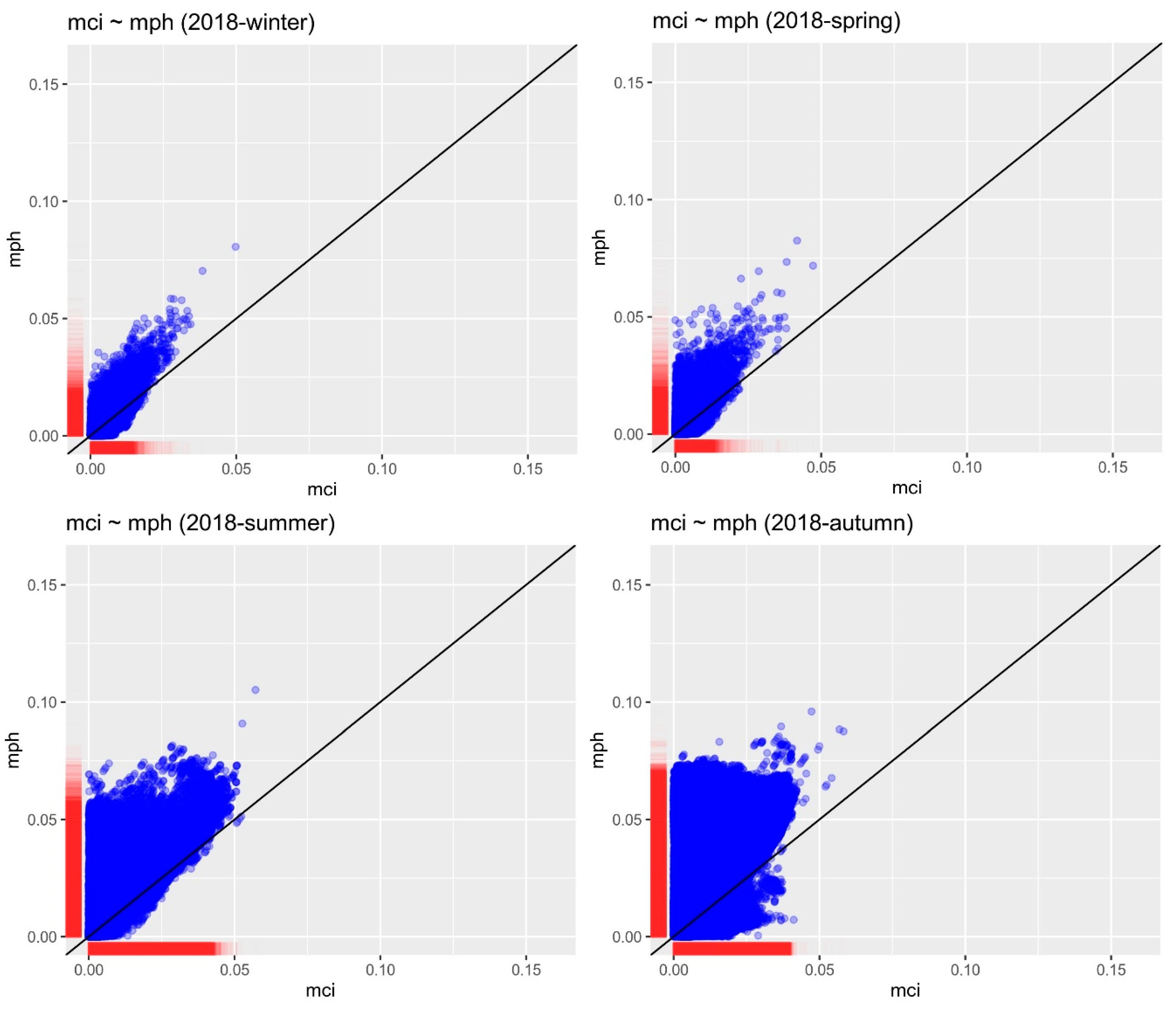
3.1. MPH and MCI Correlation

The MPH and MCI algorithms were applied to all datasets in order to visually and statistically compare the results. Both indices appeared to work well, as they shared some common features. For the detection of chl-a, both algorithms used the wavelengths at 665 nm and 705 nm.

Table 1. Pearson’s r correlation coefficient per year and per season.

	Annual	Winter	Spring	Summer	Autumn
2016	0.92	0.88	0.66	0.95	0.70
2017	0.75	0.77	0.92	0.89	0.48
2018	0.82	0.81	0.62	0.85	0.65

presents the overall annual and per season relationship between the MCI and MPH, according to Pearson’s r correlation coefficient.

All of the coefficients showed a strong positive correlation between the MPH and the MCI. The strong correlations are also evident in the scatterplots (Figure A1, Figure A2 and Figure A3). This was quite expected, as both algorithms are based on chl-a scattering peaks above a specific baseline even if they can provide divergent results in some cases. Despite the correlation and the strong positive relationship between these algorithms, the MPH was further analyzed due to the provided algorithms that correlate the MPH index with the chl-a concentrations. Furthermore, based on previous research, the MPH is more suitable for the estimation of the chl-a concentration across different trophic ranges and water types [39]. Finally, from visual inspection of our products, it was observed that, for specific days, the MCI values were negative. This could happen due to a shift of the chl-a reflectance peak to the longer wavelengths; a response that has been also observed for the FLH algorithm within previous research [40]. Nevertheless, the most likely reason for the negative MCI in our study area is the very dense surface cyanobacterial scums. The reflectance of these dense scums is increased in wavelengths beyond 700 nm and is similar to the reflectance response of aquatic macrophytes [41].

3.2. MPH and Chl-A Concentration

MPH mapping revealed that the intense chlorophyll activity is mainly observed in the summer and autumn months and, in particular, the month of October, indicating that this is an outbreak season for eutrophication. On the contrary, we could argue that winter and spring months are observed to be inactive regarding the identification and distribution of high MPH values (Figure 4). During the inactive period, the MPH index is low throughout the lake (i.e., 14 April 2016, 09 April 2017, and 12 April 2018 of Figure 4). However, in the vicinity of the coast, due to the adjacency effect, the reflectances of the pixels are influenced by the land, resulting in non-confident results for these specific areas [42]. On the other hand, during an outbreak (i.e., 14 October 2016, 09 October 2017, and 09 October 2018 of Figure 4), the spatial distribution of the MPH index varies. From visual inspection of all 65 images, the higher values of MPH are concentrated on the east side of the lake. The major contributors of high chl-a concentrations are the agricultural fertilizers and the light industrial and urban wastes that inflow through inflow points at the south side of the lake [2].

According to the empirical model described above, the highest concentration of chl-a reached 257 µg/L. In Figure 5, we can see the outbreak of the phenomenon during September and October of 2017, as these were the only available dates with images containing no clouds for this specific outbreak event. Spring outbreaks last for a shorter time and present a lower concentration of chl-a. Figure 6 shows a spring–early summer outbreak episode, during the period from 23 March 2017 to 28 June 2017. At the beginning of this period the concentration did not present any spatial variation and was equal to approximately 20 μg/L, rising to 30 μg/L on 09 April 2017. From 02/05, an outbreak took place with maximum values at the west part of the lake, approximately 50 μg/L, while two cores of high values were formed in mid May, with concentrations up to 170 μg/L. At 01/06, one core of high value remained in the east part, with approximately 130 μg/L. The next available clear image is from 28/06, where the concentrations were similar to the whole lake, at approximately 20 μg/L.

From the results of the two periods presented above, it is clear that there is a hypertrophic state in the lake. Moreover, we can see the sensor’s suitability to monitor an event with high spatial and temporal resolution, even if a significant number of images were discarded due to clouds. Apart from the adjacency effect that is described above, some images were contaminated by stripe noise. Stripe noise removal is an active research problem, and the solutions applied may lead to a possible degradation of structural details with the same frequencies as stripes related to the useful signal [43,44]. Previous research has shown that the stripes amount, on average, to between ±7 Digital Numbers (DN) and ±4 DN for the bands 4, 8, and 11 of the MSI, which equals 0.0007 and 0.0004 TOA respectively [45]. Thus, a periodic stripe noise removal filter was not applied; however, we maintain a high degree of confidence in this kind of analysis. External factors may also play an import role in water eutrophication and in its spatial distribution, such as weather conditions, i.e., temperature, humidity, wind speed, and direction [46].

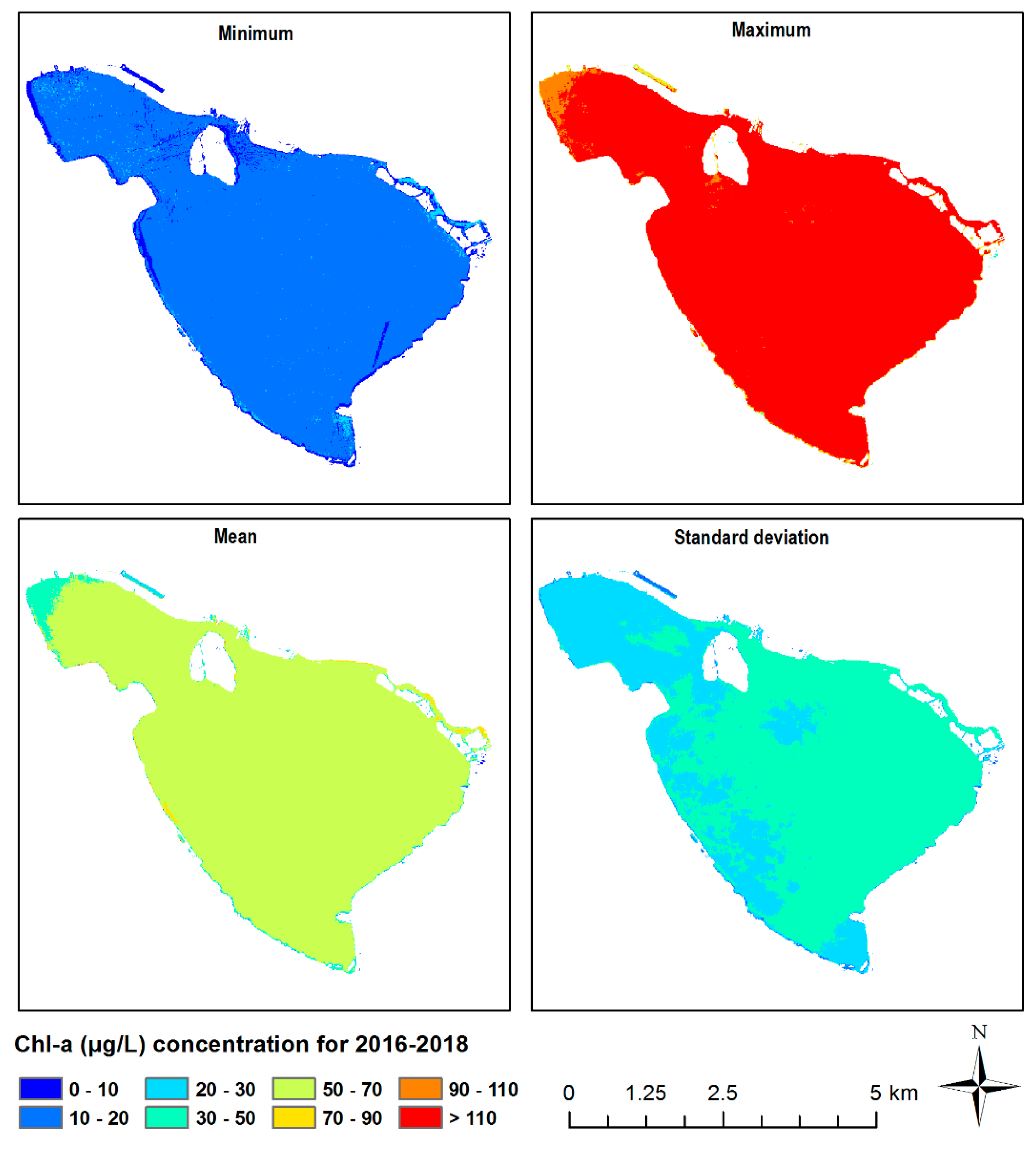
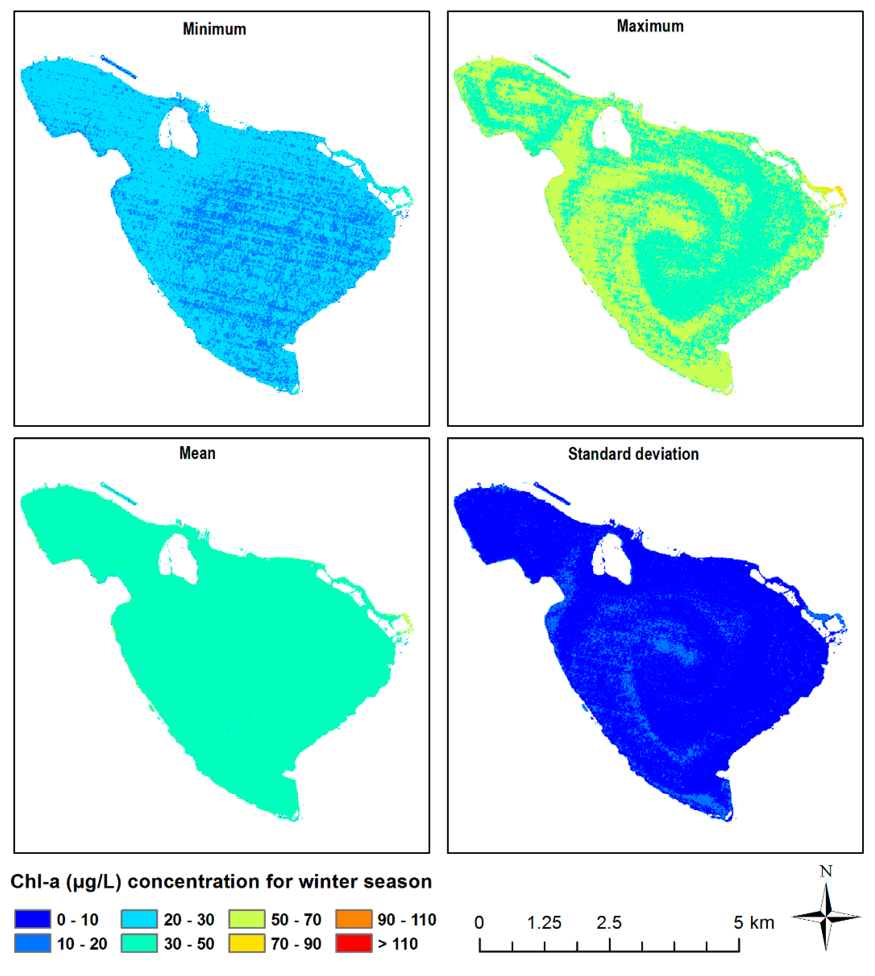
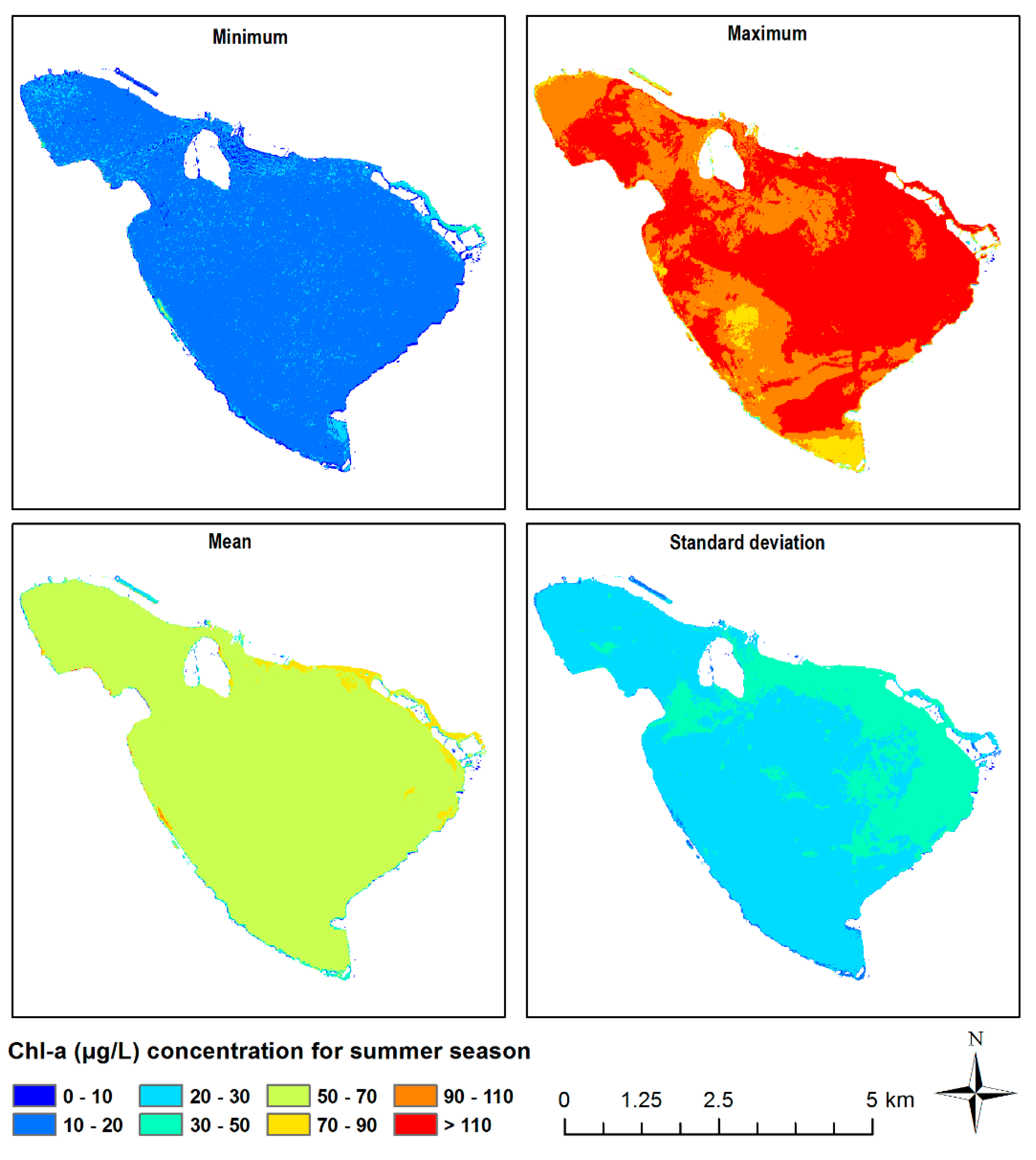
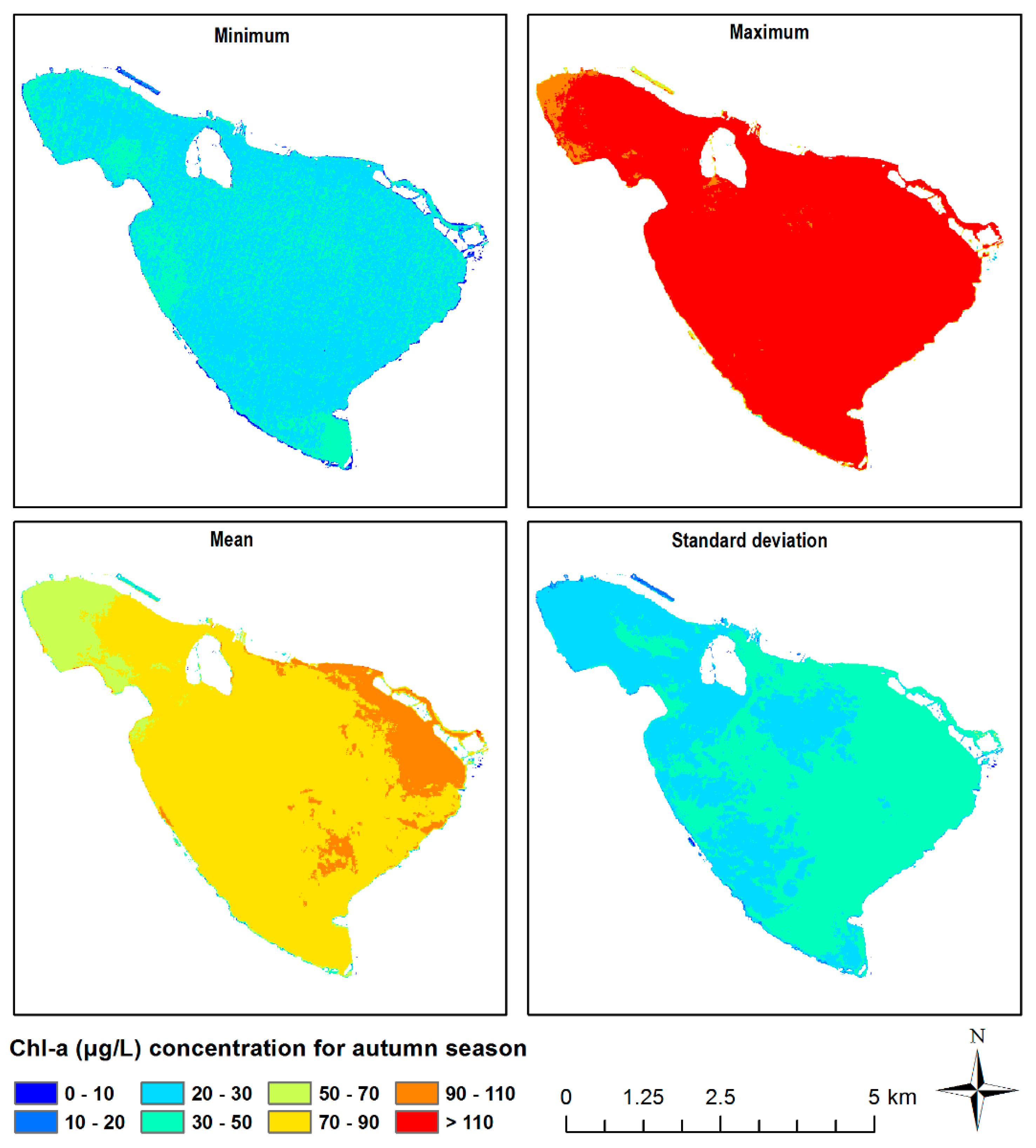
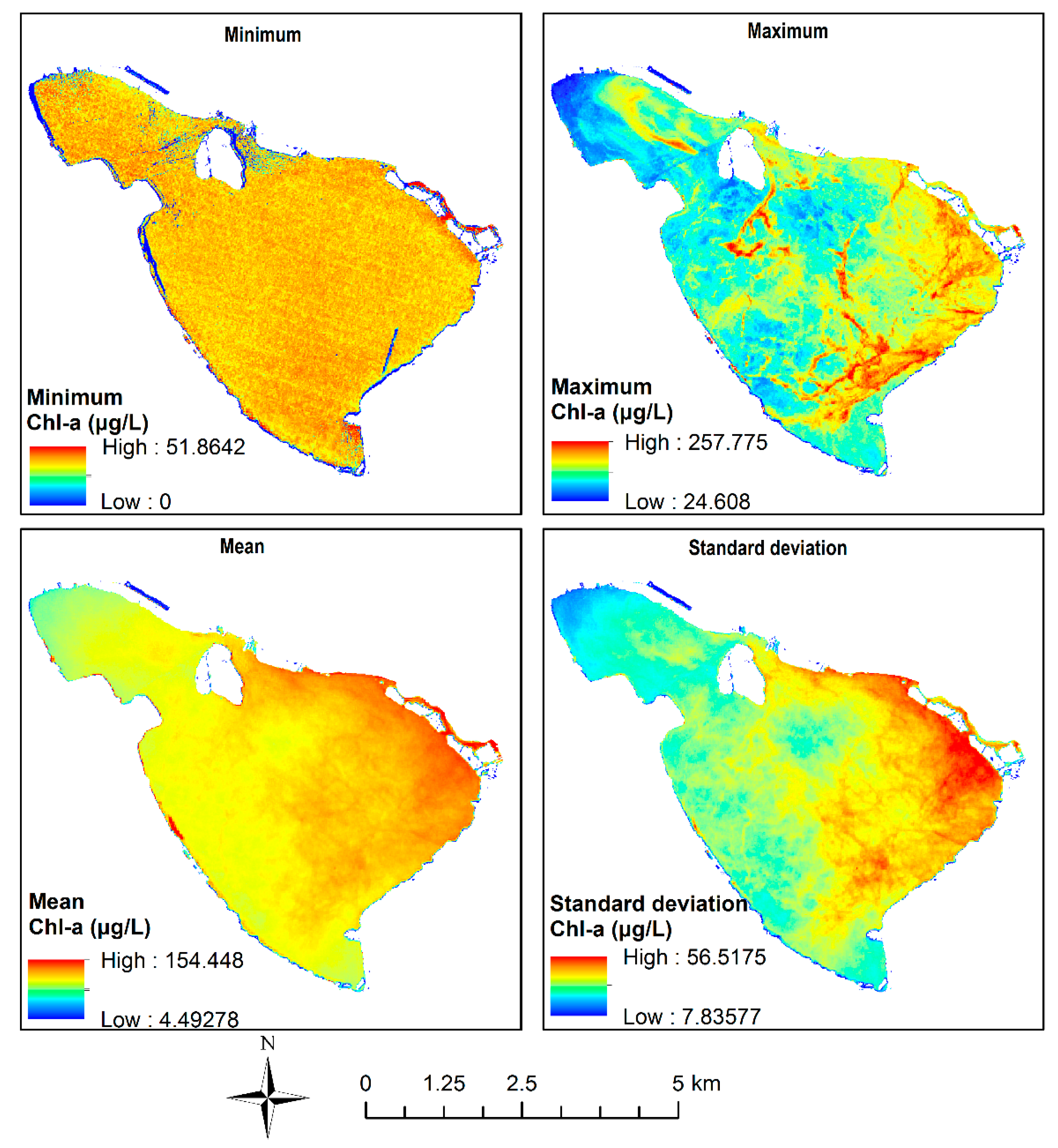
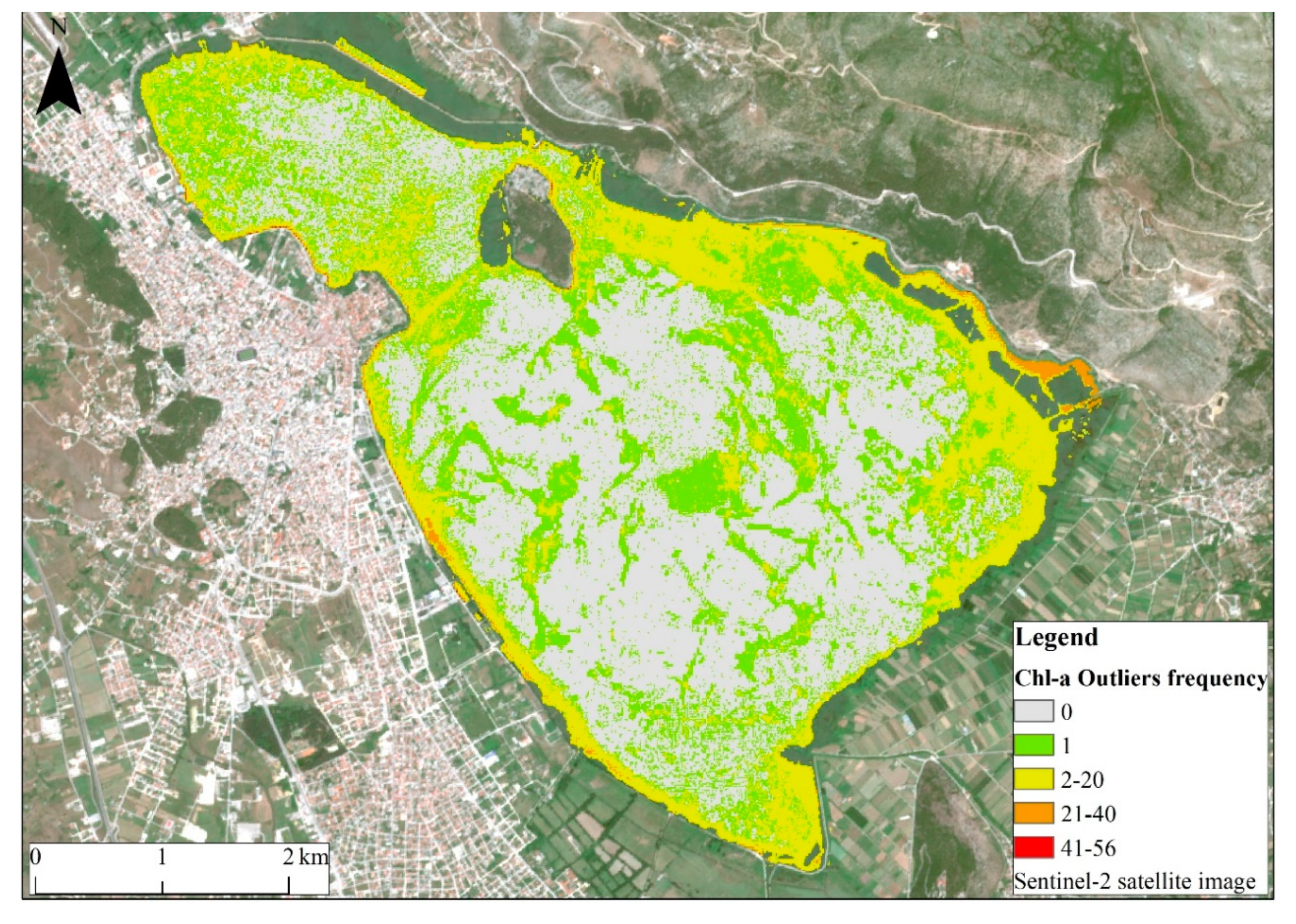
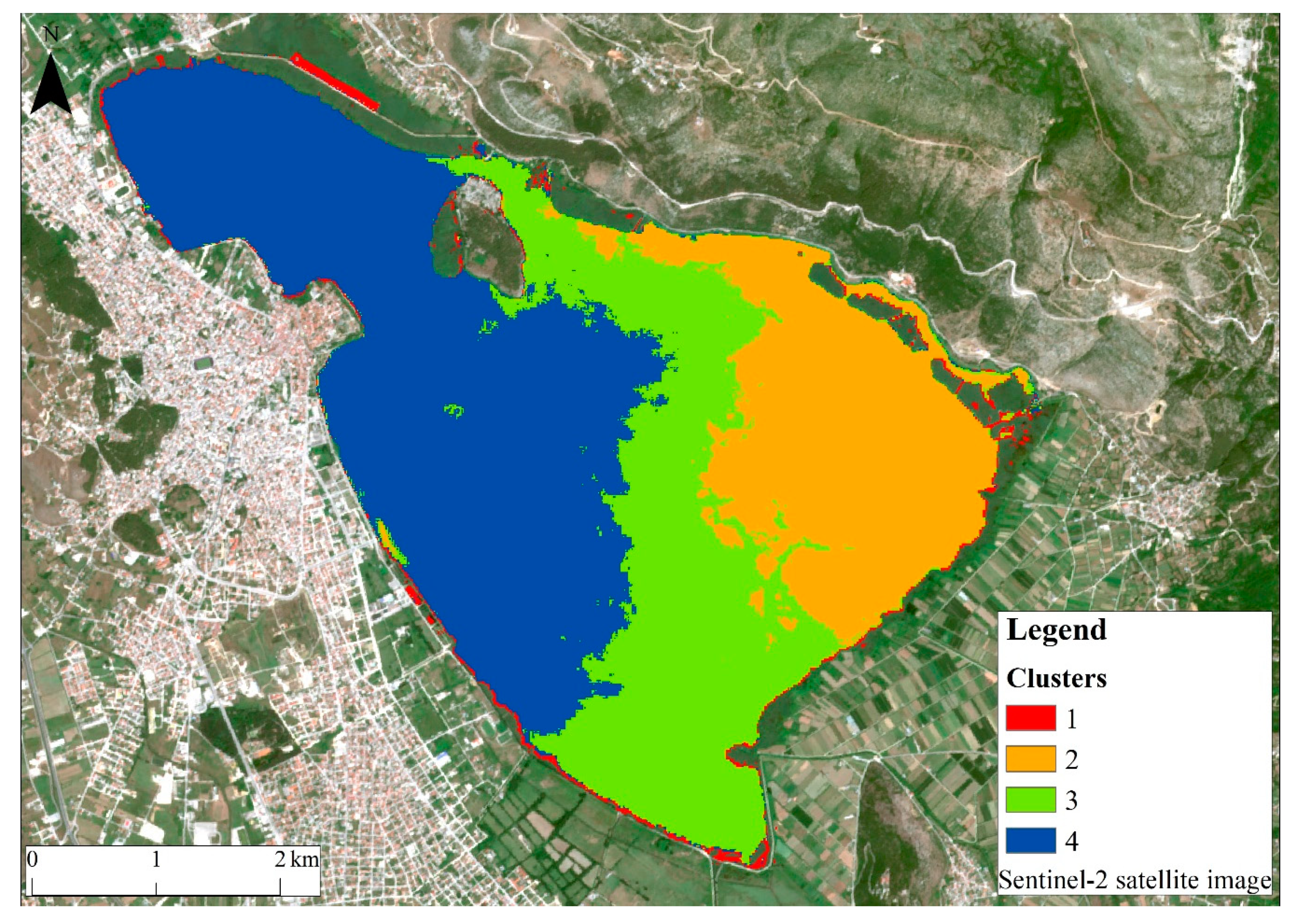
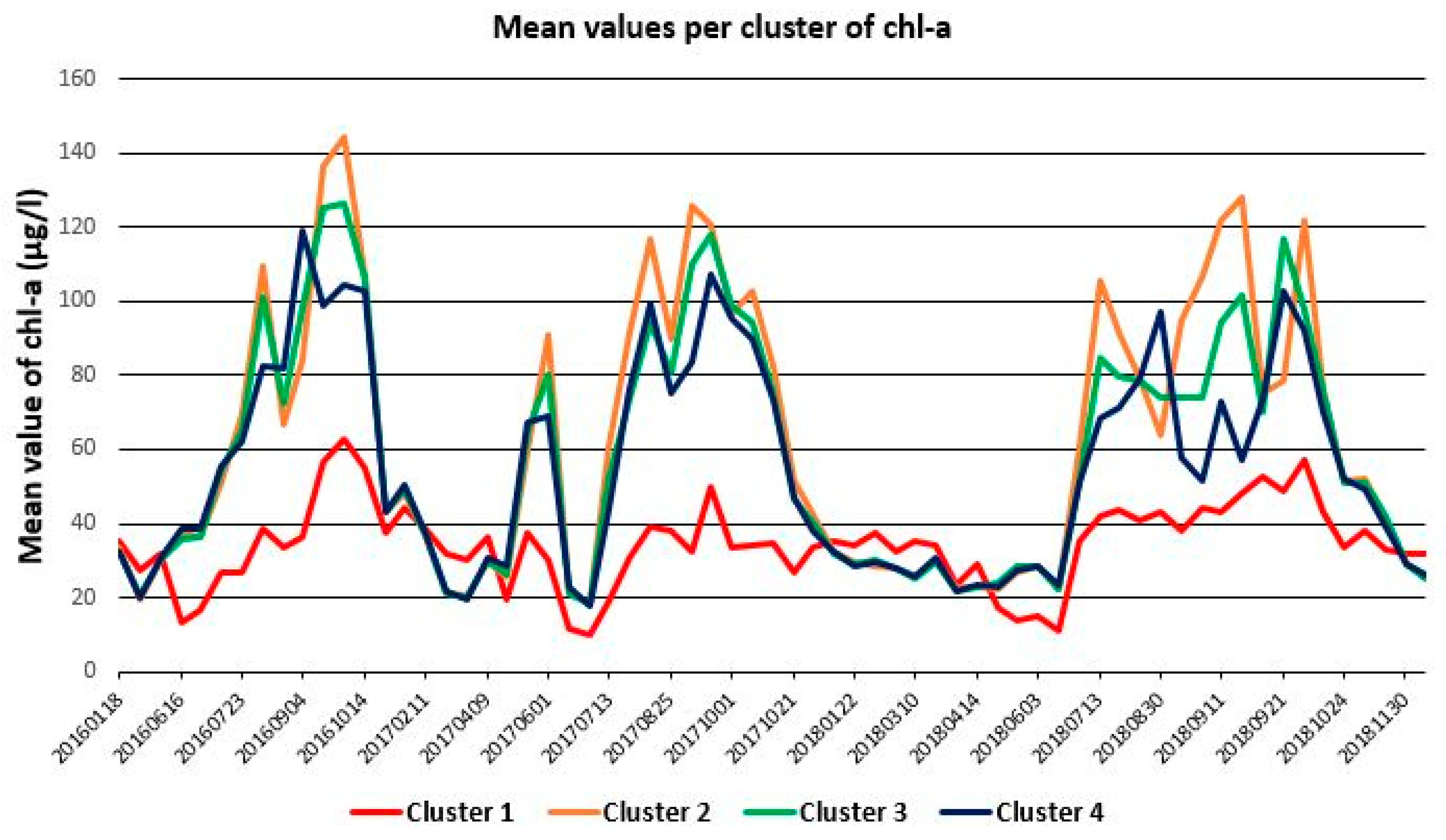
3.3. Statistical Analysis of Chl-A Concentration

The next step in our study was to perform spatial and temporal statistical analysis of the distribution of the chl-a in the study area. For all of the concentration maps, we calculated the minimum, maximum, mean, and standard deviation for each pixel (Figure 7). The minimum values appeared mostly at the north-west coast where the lake is adjacent to the urban area. Furthermore, some artifacts were observed due to the strip noise of the bands that are taken into consideration for the calculation of the MPH. On the other hand, the maximum values were observed at the east and south–east coast with values reaching up to 260 µg/L, which also confirms the interpretation of the high concentration of chl-a in the specific area from crops and pollutant sources. The mean chl-a values show an indicative 2 year situation in the lake. The average concentration values, according to trophic classification by Serwan et. al. [47], determine the water quality and show that the lake is hypertrophic, as the main values of the concentration levels reached 56 µg/L.

The standard deviations indicate that the largest rate of changes and distribution of chl-a were in the southeast bank of the lake. Moreover, the comparison of the mean and standard deviation indicates that there was a spatial agreement between them. The visualization of the maps of Figure 7 is based on a stretched color ramp according to the minimum and maximum values of each raster. We applied this scheme in order to emphasize the relative spatial distribution of high and low values. Figure A4, Figure A5, Figure A6, Figure A7 and Figure A8 present the same statistics with a classified color scheme for the whole time period and per season. This color scheme highlights the absolute concentration values rather than the relative spatial distribution.

One of the main outputs of the current workflow was the calculation of the outliers, i.e., to identify the areas that have high concentrations. For each date, each pixel was classified as an outlier or not according the quartiles of the corresponding image and the method described above. The 65 binary results were summed in order to identify the frequency of pixels classified as outliers (Figure 8). The majority of the area did not present any extreme high values of concentration for the study period. Approximately 6 km² of the lake presented, only once, an extreme concentration away from the coast. Higher frequencies of extreme values were observed close to the coast, mainly at the south and east sides of the lake. The pixels adjacent to land may suffer from the adjacency effect described above. The two cores of pixels in the class 21–40 observed at the east and west of the lake are due to the aquatic vegetation observed in the summer and autumn seasons, and the pixels with frequency 2–20 are due to extreme concentrations of chl-a from the agricultural activities that take place.

Finally, an ISODATA clustering was applied to the dataset in order to identify any spatial and temporal trends regarding the concentration of chl-a. The optimal number of clusters to group the dataset, regarding the homogeneity/compactness of the clusters, was four, according to its frequency among all indices of the NbClust R package (Figure 9). A measure of the total variance in our dataset that is explained by the performed clustering is the ratio of the between sum of squares (BSS) and the total sum of squares (TSS), which was 74.01% for the four groups.

Figure 10 presents the clusters, while Figure 11 presents the temporal variation of the mean values of each cluster. The first class includes area that does not show temporal peaks of the variation but balanced and relative low concentrations, with an average below 60 μg/L. The pixels of this cluster are few and are located at the borders of the lake. It is likely that this cluster includes pixels that suffer from the adjacency effect.

The peaks for all other classes were observed during the autumn–winter months of each year, following the same seasonal and annual patterns. Class 2 had the highest chl-a values observed at the east part of the lake. For the year 2016, the chl-a mean values were marginally higher and reached up to 140 μg/L, while in 2017 and 2018, they reach 120 µg/L. The other three clusters followed the same distribution pattern of class 2, however in lower concentration levels. Class 4 was observed to concentrate at the northwest side, presenting the lower concentrations, and class 3 was observed from the north-east part through the south part of the lake. In general, we observed a spatial segmentation of the lake in three groups of concentrations according to the three-year remote sensing data.

4. Conclusions

In conclusion, the three-year study of the remotely sensed data revealed that Pamvotis’ state is mainly eutrophic, with a specific period of outbreak for the phenomenon.

In this paper, two significant chl-a detection algorithms, the MPH and the MCI were estimated in eutrophic condition waters, to discuss the Sentinel-2 capabilities and limitations. Many studies have indicated that both algorithms can detect chl-a and aquatic vegetation; our study, with the estimation of Pearson’s r between the MCI and MPH finds the same conclusion. The MPH was further correlated with chl-a concentration based on a model derived within another research for another study area in Lithuania [18]. On the other hand, as the present study did not include any in situ measurements, the values of the estimated chl-a concentrations need thorough considerations. Nevertheless, for a comparison to our findings, the most recent to our study in situ measurements are provided by the Management Body of Pamvotis lake. According to this study, the average annual value of chl-a is 46.6 μg/L, with a maximum value of 298.1 μg/L (June) and a minimum value of 4.9 μg/L (April) for the time period 2010–2011 [48]. Older in situ measurements are summarized in previous research by Kagalou et al. (2008) [23].

In the spatial analysis of chl-a distribution, we conclude that the highest levels accumulate at the south and south-east shore of the lake. The systematic detection of extreme chl-a values (maximum outliers) may be influenced by temporal factors in the aquatic vegetation, due to the growth cycle or exposure, due to water level alterations.

The main sources of pollution in the lake are the nearby urban area and agricultural land [49], where human activities increase the wastes in the water, resulting in the development of phytoplankton communities [2]. A waste water treatment plant has operated since the mid-1990s; however, illegal disposal of untreated human and industrial wastes unfortunately still occurs. These wasters and the intensive usage of fertilizers cause a reduction in water quality.

Our results can provide some guidance to lake managers in order to identify areas prone to eutrophication and coastal zones that may influence the lake through water canals. Further improvement of the analysis should include the atmospheric correction of the data and the exclusion of areas that are not covered by in-water vegetation or that not have their waterbed exposed at any time within an annual cycle. The newer Sentinel-3 sensor can also be evaluated, given its 10 bands in the range of 665–865 nm, despite its low spatial resolution of 300 m. Finally, in situ water parameters should be retrieved and correlated with the Sentinel-2 data, in order to build an algorithm for more accurate results.

References

1. Chaplin, M.F. Water: Its importance to life. Biochem. Mol. Biol. Educ. 2001, 29, 54–59. [Google Scholar] [CrossRef]
2. Kagalou, I.; Tsimarakis, G.; Paschos, I. Water chemistry and biology in a shallow lake (Lake pamvotis- Greece). present state and perspectives. Glob. Nest J. 2001, 3, 85–94. [Google Scholar]
3. Khan, M.N.; Mohammad, F. Eutrophication: Challenges and solutions. In Eutrophication: Causes, Consequences and Control; Springer: Dordrecht, The Netherlands, 2014; ISBN 9789400778146. [Google Scholar]
4. Jensen, J.R. Remote Sensing of the Environment: An Earth Resource Perspective, 2nd ed.; Pearson Education Limited: Harlow, UK, 2014; ISBN 9780131889507. [Google Scholar]
5. Hovis, W.A.; Clark, D.K.; Anderson, F.; Austin, R.W.; Wilson, W.H.; Baker, E.T.; Ball, D.; Gordon, H.R.; Mueller, J.L.; El-Sayed, S.Z.; et al. Nimbus-7 coastal zone color scanner: System description and initial imagery. Science 1980, 210, 60–63. [Google Scholar] [CrossRef]
6. Kravitz, J.; Matthews, M.; Bernard, S.; Griffith, D. Application of Sentinel 3 OLCI for chl-a retrieval over small inland water targets: Successes and challenges. Remote Sens. Environ. 2020, 237, 111562. [Google Scholar] [CrossRef]
7. Cazzaniga, I.; Bresciani, M.; Colombo, R.; Della Bella, V.; Padula, R.; Giardino, C. A comparison of Sentinel-3-OLCI and Sentinel-2-MSI-derived Chlorophyll- a maps for two large Italian lakes. Remote Sens. Lett. 2019, 10, 978–987. [Google Scholar] [CrossRef]
8. Kondraju, T.T.; Rajan, K.S. Water Quality in Inland Water Bodies: Hostage to the Intensification of Anthropogenic Land Uses. J. Indian Soc. Remote Sens. 2019, 47, 1865–1874. [Google Scholar] [CrossRef]
9. Watanabe, F.; Alcântara, E.; Bernardo, N.; de Andrade, C.; Gomes, A.C.; do Carmo, A.; Rodrigues, T.; Rotta, L.H. Mapping the chlorophyll-a horizontal gradient in a cascading reservoirs system using MSI Sentinel-2A images. Adv. Space Res. 2019, 64, 581–590. [Google Scholar] [CrossRef]
10. Xu, M.; Liu, H.; Beck, R.; Lekki, J.; Yang, B.; Shu, S.; Kang, E.L.; Anderson, R.; Johansen, R.; Emery, E.; et al. A spectral space partition guided ensemble method for retrieving chlorophyll-a concentration in inland waters from Sentinel-2A satellite imagery. J. Great Lakes Res. 2019, 45, 454–465. [Google Scholar] [CrossRef]
11. Toming, K.; Kutser, T.; Laas, A.; Sepp, M.; Paavel, B.; Nõges, T. First experiences in mapping lakewater quality parameters with sentinel-2 MSI imagery. Remote Sens. 2016, 8, 640. [Google Scholar] [CrossRef] [Green Version]
12. Ha, N.T.T.; Thao, N.T.P.; Koike, K.; Nhuan, M.T. Selecting the best band ratio to estimate chlorophyll-a concentration in a tropical freshwater lake using sentinel 2A images from a case study of Lake Ba Be (Northern Vietnam). ISPRS Int. J. Geo.Inf. 2017, 6, 290. [Google Scholar] [CrossRef]
13. Dörnhöfer, K.; Klinger, P.; Heege, T.; Oppelt, N. Multi-sensor satellite and in situ monitoring of phytoplankton development in a eutrophic-mesotrophic lake. Sci. Total Environ. 2018, 612, 1200–1214. [Google Scholar] [CrossRef] [PubMed]
14. Poddar, S.; Chacko, N.; Swain, D. Estimation of Chlorophyll-a in Northern Coastal Bay of Bengal Using Landsat-8 OLI and Sentinel-2 MSI Sensors. Front. Mar. Sci. 2019, 6, 598. [Google Scholar] [CrossRef]
15. Binding, C.E.; Greenberg, T.A.; Bukata, R.P. The MERIS Maximum Chlorophyll Index; its merits and limitations for inland water algal bloom monitoring. J. Great Lakes Res. 2013, 39, 100–107. [Google Scholar] [CrossRef]
16. Gower, J.; King, S.; Goncalves, P. Global monitoring of plankton blooms using MERIS MCI. Proc. Int. J. Remote Sens. 2008, 29, 3209–6216. [Google Scholar] [CrossRef]
17. Mollaee, S. Estimation of Phytoplankton Chlorophyll-a Concentration in the Western Basin of Lake Erie Using Sentinel-2 and Sentinel-3 Data. Master’s Thesis, University of Waterloo, Waterloo, ON, Canada, 2018. [Google Scholar]
18. Grendaitė, D.; Stonevičius, E.; Karosienė, J.; Savadova, K.; Kasperovičienė, J. Chlorophyll-a concentration retrieval in eutrophic lakes in Lithuania from Sentinel-2 data. Geol. Geogr. 2018, 4, 15–28. [Google Scholar] [CrossRef]
19. Matthews, M.W.; Bernard, S.; Robertson, L. An algorithm for detecting trophic status (chlorophyll-a), cyanobacterial-dominance, surface scums and floating vegetation in inland and coastal waters. Remote Sens. Environ. 2012, 124, 637–652. [Google Scholar] [CrossRef]
20. Gower, J.F.R.; Doerffer, R.; Borstad, G.A. Interpretation of the 685nm peak in water-leaving radiance spectra in terms of fluorescence, absorption and scattering, and its observation by MERIS. Int. J. Remote Sens. 1999, 20, 1771–1786. [Google Scholar] [CrossRef]
21. Soriano-González, J.; Angelats, E.; Fernández-Tejedor, M.; Diogene, J.; Alcaraz, C. First results of phytoplankton spatial dynamics in two NW-Mediterranean bays from chlorophyll-A estimates using Sentinel 2: Potential implications for aquaculture. Remote Sens. 2019, 20, 1756. [Google Scholar] [CrossRef] [Green Version]
22. Elhag, M.; Gitas, I.; Othman, A.; Bahrawi, J.; Gikas, P. Assessment of water quality parameters using temporal remote sensing spectral reflectance in arid environments, Saudi Arabia. Water Switzerland 2019, 11, 556. [Google Scholar] [CrossRef] [Green Version]
23. Kagalou, I.; Papastergiadou, E.; Leonardos, I. Long term changes in the eutrophication process in a shallow Mediterranean lake ecosystem of W. Greece: Response after the reduction of external load. J. Environ. Manag. 2008, 87, 497–506. [Google Scholar] [CrossRef]
24. Papatheodorou, G.; Demopoulou, G.; Lambrakis, N. A long-term study of temporal hydrochemical data in a shallow lake using multivariate statistical techniques. Ecol. Model. 2006, 193, 759–776. [Google Scholar] [CrossRef]
25. Papastergiadou, E.; Kagalou, I.; Stefanidis, K.; Retalis, A.; Leonardos, I. Effects of anthropogenic influences on the trophic state, land uses and aquatic vegetation in a shallow Mediterranean lake: Implications for restoration. Water Resour. Manag. 2010, 24, 415–435. [Google Scholar] [CrossRef]
26. Romero, J.R.; Kagalou, I.; Imberger, J.; Hela, D.; Kotti, M.; Bartzokas, A.; Albanis, T.; Evmirides, N.; Karkabounas, S.; Papagiannis, J.; et al. Seasonal water quality of shallow and eutrophic Lake Pamvotis, Greece: Implications for restoration. Hydrobiologia 2002, 474, 91–105. [Google Scholar] [CrossRef]
27. Yannopoulos, S.; Kaloyannis, H. Water quality modelling of the Pamvotis lake (Greece) using the wasp mathematical model. In Proceedings of the 2008 International Conference of Protection and Restoration of the Environment IX, Kefalonia Island, Greece, 30 June–03 July 2008. [Google Scholar]
28. Hadjisolomou, E.; Stefanidis, K.; Papatheodorou, G.; Papastergiadou, E. Assessing the contribution of the environmental parameters to eutrophication with the use of the “PaD” and “PaD2” methods in a hypereutrophic lake. Int. J. Environ. Res. Public Health 2016, 13, 764. [Google Scholar] [CrossRef] [PubMed] [Green Version]
29. Hadjisolomou, E.; Stefanidis, K.; Papatheodorou, G.; Papastergiadou, E. Evaluating the contributing environmental parameters associated with eutrophication in a shallow lake by applying artificial neural networks techniques. Fresenius Environ. Bull. 2017, 26, 3200–3208. [Google Scholar]
30. Kati, V.; Mani, P.; von Helversen, O.; Willemse, F.; Elsner, N.; Dimopoulos, P. Human land use threatens endemic wetland species: The case of Chorthippus lacustris (La Greca and Messina 1975) (Orthoptera: Acrididae) in Epirus, Greece. J. Insect Conserv. 2006, 10, 65–74. [Google Scholar] [CrossRef]
31. Chiotelli, E.P. Evaluation of the Effects of Irrigation and Drainage Practices on the Landscape of Lake Pamvotis, Ioannina: Implications for Landscape Management in the Context of Sustainability. Agric. Agric. Sci. Procedia 2015, 4, 201–210. [Google Scholar] [CrossRef]
32. McFeeters, S.K. The use of the Normalized Difference Water Index (NDWI) in the delineation of open water features. Int. J. Remote Sens. 1996, 17, 1425–1432. [Google Scholar] [CrossRef]
33. Illian, J.; Penttinen, A.; Stoyan, H.; Stoyan, D. Statistical Analysis and Modelling of Spatial Point Patterns; John Wiley and Sons: New York, NY, USA, 2008; ISBN 9780470725160. [Google Scholar]
34. Whaley, D.L. The Interquartile Range: Theory and Estimation. Electronic Theses and Dissertations. Bachelor’s Thesis, East Tennessee State University, Johnson City, TN, USA, 2005. [Google Scholar]
35. Memarsadeghi, N.; Mount, D.M.; Netanyahu, N.S.; Le Moigne, J. A fast implementation of the isodata clustering algorithm. Proc. Int. J. Comput. Geom. Appl. 2007, 17, 71–103. [Google Scholar] [CrossRef]
36. Jain, A.K. Data clustering: 50 years beyond K-means. Pattern Recognit. Lett. 2010, 31, 651–666. [Google Scholar] [CrossRef]
37. Li, B.; Zhao, H.; Lv, Z.H. Parallel ISODATA clustering of remote sensing images based on MapReduce. In Proceedings of the 2010 International Conference on Cyber-Enabled Distributed Computing and Knowledge Discovery, Huangshan, China, 10–12 October 2010. [Google Scholar]
38. Charrad, M.; Ghazzali, N.; Boiteau, V.; Niknafs, A. NbClust: An R Package for Determining the Relevant Number of Clusters in a Data Set. J. Stat. Softw. 2014, 61, 1–36. [Google Scholar] [CrossRef] [Green Version]
39. Matthews, M.W.; Odermatt, D. Improved algorithm for routine monitoring of cyanobacteria and eutrophication in inland and near-coastal waters. Remote Sens. Environ. 2015, 156, 374–382. [Google Scholar] [CrossRef]
40. Tao, B.; Mao, Z.; Pan, D.; Shen, Y.; Zhu, Q.; Chen, J. Influence of bio-optical parameter variability on the reflectance peak position in the red band of algal bloom waters. Ecol. Inform. 2013, 16, 17–24. [Google Scholar] [CrossRef]
41. Liang, Q.; Zhang, Y.; Ma, R.; Loiselle, S.; Li, J.; Hu, M. A MODIS-based novel method to distinguish surface cyanobacterial scums and aquatic macrophytes in Lake Taihu. Remote Sens. 2017, 9, 133. [Google Scholar] [CrossRef] [Green Version]
42. Sterckx, S.; Knaeps, E.; Ruddick, K. Detection and correction of adjacency effects in hyperspectral airborne data of coastal and inland waters: The use of the near infrared similarity spectrum. Int. J. Remote Sens. 2011, 32, 6479–6505. [Google Scholar] [CrossRef]
43. Chang, Y.; Yan, L.; Wu, T.; Zhong, S. Remote Sensing Image Stripe Noise Removal: From Image Decomposition Perspective. IEEE Trans. Geosci. Remote Sens. 2016, 32, 6479–6505. [Google Scholar] [CrossRef]
44. Chen, Y.; Huang, T.Z.; Zhao, X.L.; Deng, L.J.; Huang, J. Stripe noise removal of remote sensing images by total variation regularization and group sparsity constraint. Remote Sens. 2017, 54, 559. [Google Scholar] [CrossRef] [Green Version]
45. Kääb, A.; Winsvold, S.H.; Altena, B.; Nuth, C.; Nagler, T.; Wuite, J. Glacier remote sensing using sentinel-2. part I: Radiometric and geometric performance, and application to ice velocity. Remote Sens. 2016, 8, 598. [Google Scholar] [CrossRef] [Green Version]
46. Xia, R.; Zhang, Y.; Critto, A.; Wu, J.; Fan, J.; Zheng, Z.; Zhang, Y. The potential impacts of climate change factors on freshwater eutrophication: Implications for research and countermeasures of water management in China. Sustainability 2016, 8, 229. [Google Scholar] [CrossRef] [Green Version]
47. Serwan, M.J.B. Trophic classification and ecosystem checking of lakes using remotely sensed information. Hydrol. Sci. J. 1996, 41, 939–957. [Google Scholar]
48. Nitas, P. Lake Pamvotis Water Monitoring Program. Available online: http://www.lakepamvotis.gr/img/monitoring/Monitoring_Nitas_P.pdf (accessed on 12 February 2020).
49. Kopsidas, O. Valuation of the External Cost Caused by the Environmental Pollution of Three Lakes in Northern Greece. J. Environ. Sci. Eng. A 2018, 7, 140–145. [Google Scholar] [CrossRef]
Figure 1. (a) The study area of Pamvotis lake, Greece and (b) the CORINE land cover types.
Ijgi 09 00143 g001
Figure 2. Peak of the reflectance in eutrophic waters at 705 nm of the electromagnetic spectrum, based on Sentinel-2 Multispectral Imager (MSI) bands.
Ijgi 09 00143 g002
Figure 3. Work flow chart. maximum chlorophyll index (MCI) and maximum peak-height (MPH).
Ijgi 09 00143 g003
Figure 4. The MPH index during active and inactive periods in Pamvotis lake. The index is dimensionless.
Ijgi 09 00143 g004
Figure 5. Outbreak of chl-a concentrations for September–October 2017. Only the available images without any cloud contamination have been processed.
Ijgi 09 00143 g005
Figure 6. Outbreak of chl-a concentrations during March–June 2017. Only the available images without any cloud contamination have been processed.
Ijgi 09 00143 g006
Figure 7. The maximum, minimum, mean, and standard deviations of Chl-a concentrations per pixel for the study period.
Ijgi 09 00143 g007
Figure 8. The frequency of chl-a maximum value outlier pixels in lake Pamvotis.
Ijgi 09 00143 g008
Figure 9. The frequency of the optimal number of clusters retrieved by 24 models.
Ijgi 09 00143 g009
Figure 10. Clustering of the 65 chl-a images.
Ijgi 09 00143 g010
Figure 11. The temporal variation of the chl-a mean values for each cluster.
Ijgi 09 00143 g011