Abstract
Georeferencing by place names (known as toponyms) is the most common way of associating textual information with geographic locations. While computers use numeric coordinates (such as longitude-latitude pairs) to represent places, people generally refer to places via their toponyms. Query by toponym is an effective way to find information about a geographic area. However, segmenting and parsing textual addresses to extract local toponyms is a difficult task in the geocoding field, especially in China. In this paper, a local spatial context-based framework is proposed to extract local toponyms and segment Chinese textual addresses. We collect urban points of interest (POIs) as an input data source; in this dataset, the textual address and geospatial position coordinates correspond at a one-to-one basis and can be easily used to explore the spatial distribution of local toponyms. The proposed framework involves two steps: address element identification and local toponym extraction. The first step identifies as many address element candidates as possible from a continuous string of textual addresses for each urban POI. The second step focuses on merging neighboring candidate pairs into local toponyms. A series of experiments are conducted to determine the thresholds for local toponym extraction based on precision-recall curves. Finally, we evaluate our framework by comparing its performance with three well-known Chinese word segmentation models. The comparative experimental results demonstrate that our framework achieves a better performance than do other models.
1. Introduction
In the information age, georeferenced information is considered to be an essential type of value-added information [1]. Our scientific, engineering, governmental, business, and political practices are all engaged in incorporating geographic information systems (GIS) to preserve and analyze georeferenced information, to discover geographic distribution patterns that support decision makers and planning [2].
Georeferencing by place names (known as toponyms) is the most common way of associating textual information with a geographic location. While computers use numeric coordinates (such as longitude-latitude pairs) to represent places, people generally refer to places via their toponyms. Toponyms are commonly used as part of a textual address to represent a geographic location, and queries to find information about a geographic area are commonly expressed as text—an approach called query by toponym. Sometimes toponym queries work seamlessly, for example, in cases where the data has been labeled with toponyms for large, well-known administrative units. However, when the desire is to find information about some smaller region that may be commonly identified with several local toponyms, or when the local toponyms are labeled differently but specify the same or similar places [3], leading to spatial-semantic ambiguities, the retrieval of relevant information using a textual query is more difficult.
For textual addresses containing local toponyms with spatial semantics, geocoding technology is considered the most significant and effective means [4] to extract the local toponyms from the text and translate them into unambiguous geographic locations. Segmenting and parsing textual addresses to extract local toponyms is an important but difficult task in the geocoding field, especially in China for the following reasons:
1. Due to the lack of unified geocoding standards, the existing Chinese textual address data are often documented inconsistently, structurally complex, and organized chaotically [5]. Thus, parsing textual addresses in China is more difficult than in countries where the textual address data are better organized;
2. Chinese is a character-based and unsegmented language (with no delimiters between words), which means that the syntax and semantics of Chinese addresses are far more complex and more difficult to parse than addresses written in segmented languages [6].
The semantic information of Chinese textual address data can be parsed by segmenting an address text into multiple address elements (including the local toponyms) for further analysis. Thus, address segmentation is a basic and crucial step in geocoding that plays an important role in the final parsing result concerning recall, accuracy rate, and operational efficiency.
Recently, natural language processing (NLP) related methods have been widely applied in applications such as information retrieval, information extraction, machine translation and so on [7]. All these methods rely on text string processing; however, when these existing methods are applied to textual address segmentation, the final result cannot meet the accuracy requirement. This problem occurs because, in contrast to other Chinese text segmentation tasks in the NLP field, a crucial step in textual address segmentation is to extract local toponyms by using textual statistical information from a raw address corpus. Previous works use only an annotated textual corpus as the input data when extracting the statistical characteristics of the text; they ignore the spatial contextual information carried by local toponyms located in small regions. However, the distribution of local toponyms in textual addresses is strongly related to their spatial locations. Therefore, ignoring these spatial characteristics leads to poor segmentation results with low precision. To improve the precision of the final results, spatial contextual information concerning the local toponyms should be provided as supplementary information during textual address segmentation procedure [8,9].
In this paper, we propose a local spatial context-based framework to extract local toponyms and segment Chinese textual addresses from urban points of interest (POIs) data. Our three major contributions are as follows.
1. We compile an urban POIs dataset in which textual addresses and geospatial coordinates have a one-to-one correspondence. This dataset can easily be used to explore the spatial distribution of local toponyms.
2. We detail an effective method for local toponym extraction that uses local spatial statistical distribution patterns to formulate some spatial statistical parameters, including spatial relatedness and degree of spatial clustering, and use them to effectively extract local toponyms for small local regions. The techniques described in this paper are generic and can be directly applied to other Chinese textual address datasets.
3. We present a computational framework that integrates both traditional NLP and our spatial statistical analysis approaches. The experimental results indicate that these integrated frameworks achieve an outstanding performance when extracting local toponyms and segmenting textual addresses exceeding that of the well-known NLP model, which is based on linguistic features alone.
In the remainder of this paper, we present the necessary background and related works in Section 2 and then describe the proposed computational framework in detail, including the input, proposed methods and output in Section 3. The results of the experiments and their evaluation are presented in Section 4, and conclusions and directions for future works are summarized in Section 5.
2. Background and Related Work
2.1. Background Knowledge
Before going into the details of the related work, the explanations of the fundamental terms “Chinese textual address”, “points of interest (POI)” and the inconsistencies of textual address description are outlined here first.
Definition 1 (Chinese textual address): A Chinese textual address A is a string of continuous text with spatial semantics and a set of address elements as defined by Equation (1):
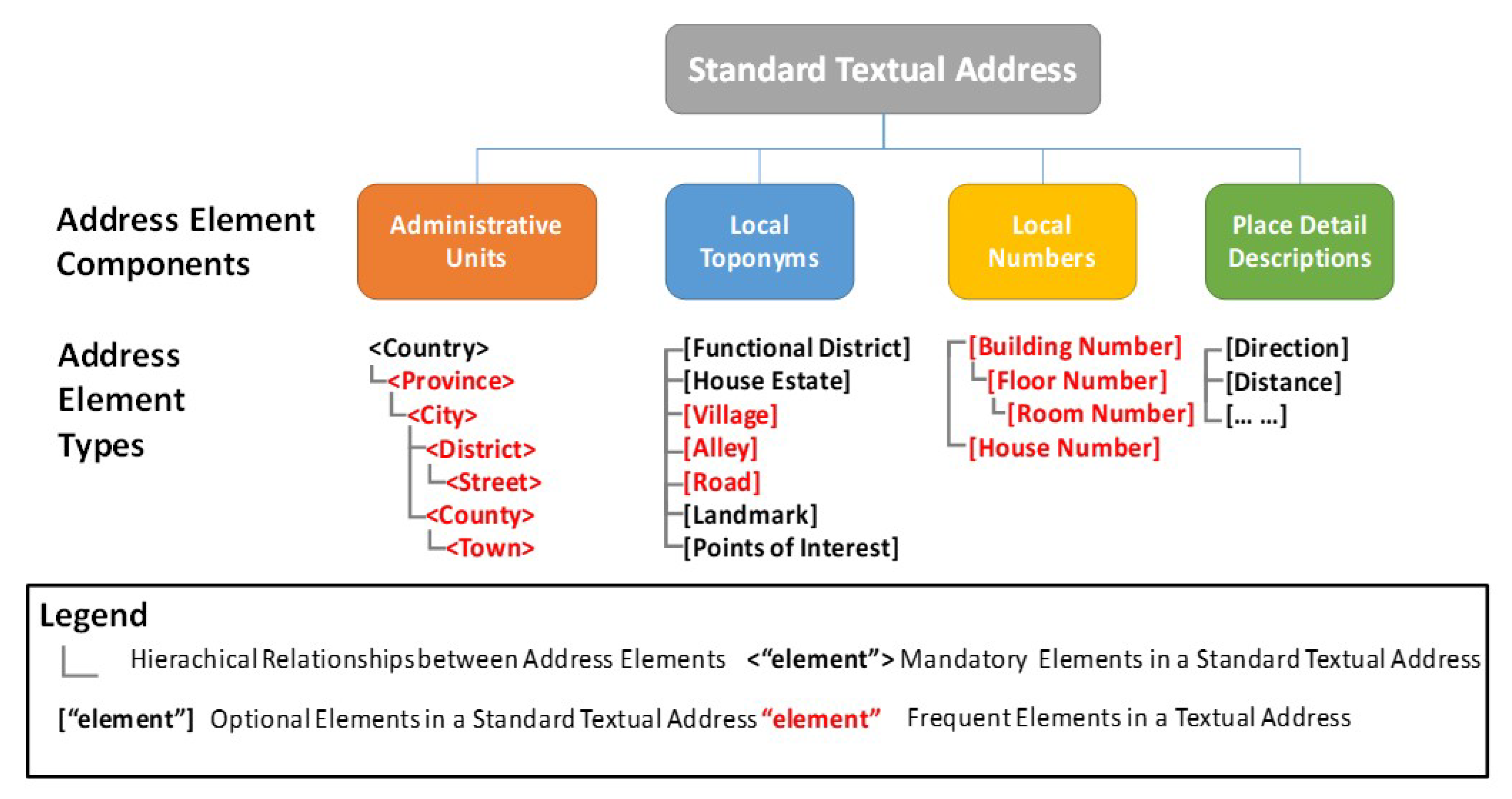
where ei and ej refer to address elements and can be regarded as the minimum spatial semantic primitive that indicates a geographical entity (such as a road, a building or a landmark and so on). R represents the spatial constraint relationship between Chinese address elements [5]. According to “Chinese National Standard GB/T 23705-2009” [10], the components and organization rules for Chinese address element types are presented in Figure 1.

Figure 1.
The components and organization rules for Chinese address element types.
A standard textual Chinese address consists of four major components: Administrative units, local toponyms, local numbers and place detail descriptions. Administrative units include all the administrative units in a standard textual address, such as a province, city, district, etc. Local toponyms include place names in a local region, such as names for a functional district or a housing estate, an alley, a road, or a village, the name of a landmark or a point of interest (POI), etc. Local numbers include numbers of geographic entities, such as the number of a building or a house, and the number of floor and room and so on. Place detail descriptions defines the relative positional information, such as the direction and distance between a described geographic entity and other referenced entities in natural language.
Definition 2 (Points of interest): A points of interest (POI) is a human construct, describing what can be found at a Location. As such a POI typically has a fine level of spatial granularity. A POI has the following attributes: a name, a current location (typically a longitude and latitude coordinate pair), a category and/or type, a unique identifier, a URI, an address (describing location or place of POI in natural language) and contact information [11].
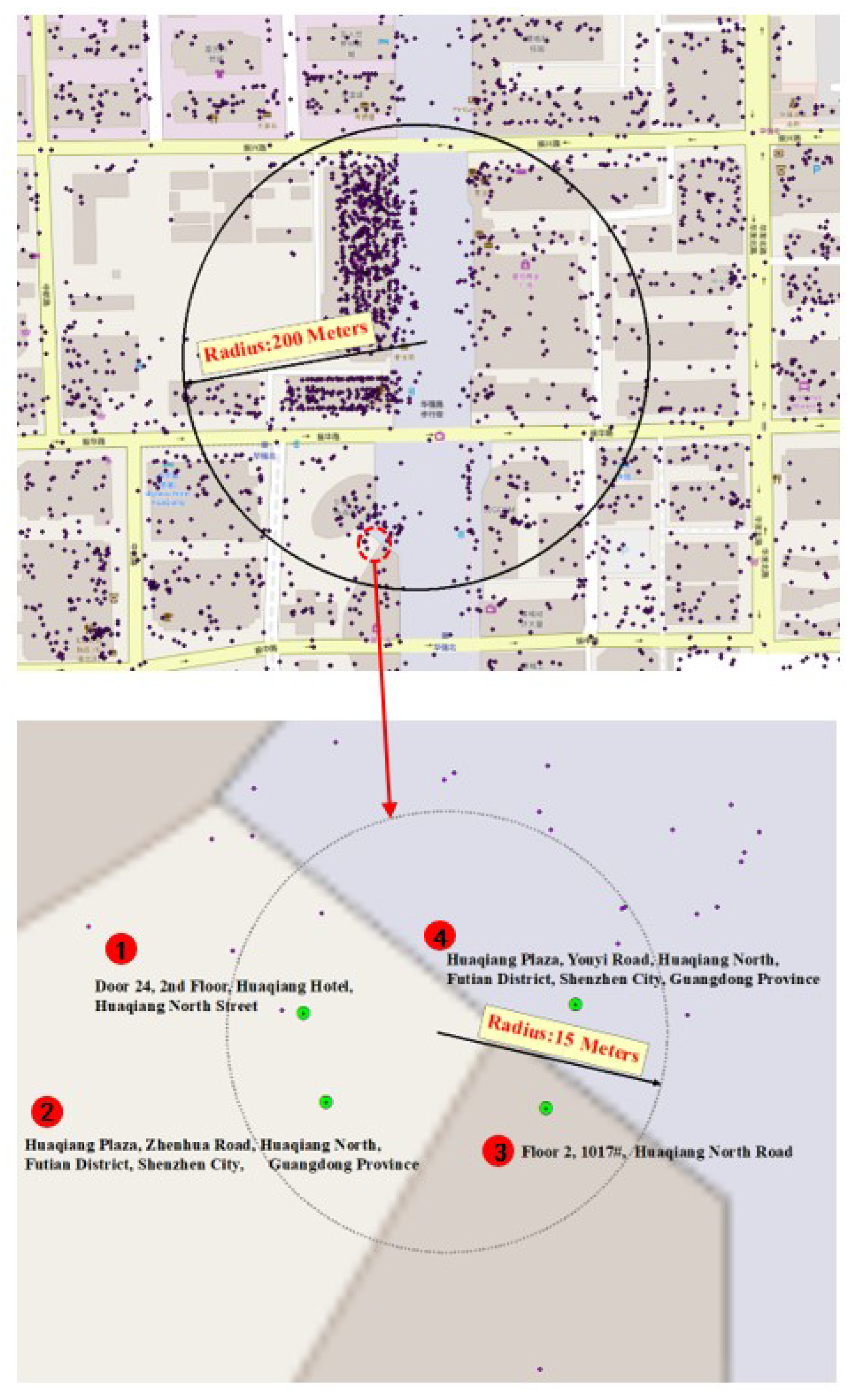
The components and organization rules for addresses provide important guidance regarding how to describe a place in natural language; however, in practice, different people and different government departments often use different forms or different address element components to describe the same place. Figure 2 shows an example of textual address description inconsistencies regarding POIs near the same building.
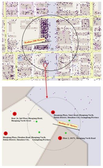
Figure 2.
An example of textual address description inconsistencies for points of interest (POIs) near the same building.
As Figure 2 shows, the textual addresses of four POIs within a 15-m radius of the same building are significantly different. The textual addresses of POI number 2 and POI number 4 are used to describe the location of the building (“Huaqiang Plaza”), but the road names are different (e.g., “Zhenhua Road” in POI number 2 and “Youyi Road” in POI number 4); moreover, the address element components included in these POIs are different: local toponyms and local numbers are included in POIs 1 and 3, while administrative units and local numbers are included in POIs 2 and 4. These differences represent description inconsistencies between different textual addresses. To resolve these inconsistencies, the address texts should be segmented into multiple address elements first.
2.2. Related Work
Chinese textual address segmentation is a specific branch of Chinese word segmentation (CWS). CWS is considered an important first step for Chinese natural language processing tasks because in contrast to space-delimited languages such as English and Spanish, written Chinese does not have explicit word boundaries [12]; thus, approaches that offer reasonable segmentation results in English or Spanish are impractical for Chinese. Previous studies have discussed how to segment Chinese textual addresses and extract toponyms from an address corpus without a lexicon, a task similar to unsupervised word segmentation in NLP [13,14]. Based on the model types used in the segmentation procedure, the developed approaches can be classified into two types: rule-based and statistics-based. In rule-based approaches, first, a predefined address model consisting of address model features of different types and the relationships between them is established. Then, the string of textual address is segmented by a maximum matching procedure [15,16,17,18]. In statistics-based approaches, pre-statistical variants, such as character frequency or cooccurrence probability, and NLP models, such as the N-gram model, hidden Markov model (HMM), conditional random field (CRF) or branch entropy, are used to segment the string of text into multiple words [19,20,21,22]. In general, the statistics-based approaches are more efficient than rule-based approaches because the strings of Chinese textual addresses are irregular; consequently, it is impossible to make a series of rules that satisfy all situations and consistently segment the textual address data correctly. However, the statistics-based approaches calculate the characteristics and patterns of the address corpus based on the textual address data itself, which is a more accurate approach than using manmade rules for textual address segmentation.
Recently, neural network models and have received considerable attention in the NLP community. Several neural models have been suggested that have achieved better performances than the traditional statistical models [23,24,25,26]. In these neural models, the processes of word segmentation and syntactic type tagging are carried out in a step by step fashion.
Although neural network models for individual word segmentation and syntactic type tagging have been intensively investigated, only a few studies have considered a neural joint model for these two tasks. Because word segmentation and syntactic type tagging are highly correlative tasks, making segmentation decisions without considering higher-level linguistic information, such as the syntactic types of the resulting words, maybe error-prone [27]. By joining the models of these two tasks, some neural models have achieved better performances than traditional statistical models on a widely adopted standard dataset [28]. These neural network models require heavy feature engineering, for example, more than 40 atomic features were designed to construct their neural network structure. The traditional statistical models, in contrast, exploit only an HMM-based or CRF-based sequence labeling framework, resulting in much lower performances than the neural network models [12].
All the above-mentioned approaches use an annotated textual corpus as the input data when extracting statistical characteristics and training models. Satisfactory segmentation results can be produced using these statistical characteristics for general text segmentation tasks. In contrast to other Chinese text segmentation tasks in the NLP field, address text segmentation is highly spatially related [29]. One crucial step in address segmentation is to extract local toponyms by using textual statistical information from a raw address corpus. Traditional NLP models use only an annotated textual corpus as the input data to extract statistical characteristics (such as word frequency, N-gram co-occurrence probability, and so on). Using only the global statistical characteristics may ignore the spatial detail information of these local toponyms, which are placed in small regions, leading to poor segmentation results with low precision. Thus, to improve the precision of the final results, the geographic locations (a latitude-longitude pair) of textual addresses should be included as supplementary input, allowing the local spatial distribution patterns of the textual addresses to be explored to extract local toponyms during the textual address segmentation procedure.
The problem of extracting local toponyms based on local spatial contextual information can be considered a spatial clustering issue. To date, various works have been introduced to cluster spatial patterns in different applications. Ref. [30] described an approach for extracting event and place semantics from Flickr geo-tagged data; Ref. [9] developed an efficient method for POI/ROI discovery using Flickr Geotagged Photos; Ref. [31] proposed an approach to spatial hotspot detection for a point data set with no geographical boundary information; Ref. [8] proposed a computational framework for harvesting local place names from geotagged housing advertisements. Spatial clustering algorithms can be classified into several categories, including (but not limited to) partitioning, hierarchical, density-based, graph-based, and grid-based approaches [32]. Because it offers several key advantages compared with other spatial clustering algorithms, density-based spatial clustering of applications with noise (DBSCAN) has been the most widely used spatial clustering algorithms for spatial point pattern discovery [33]. DBSCAN can discover point clusters and eliminate noises efficiently. Besides, it requires no prior knowledge (or estimation) of the number of clusters. The idea of using a scanning circle centered at each point with a search radius (Eps) to find at least MinPts points as a criterion for deriving local density is both understandable and sufficient for exploring isotropic spatial point patterns. Based on DBSCAN, several studies have proposed improved clustering methods such as ST-DBSCAN, which considers spatial, nonspatial and temporal values [34], P-DBSCAN, which clusters points that adopt nonduplicated owners [35], C-DBSCAN, which sets the constraints of background knowledge at the instance-level [36] and C-DBSCANO, which sets geographical knowledge constraints by combining the C-DBSCAN method and an ontology [37]. However, all of these algorithms use distance as the primary clustering criterion, and they assume that the observed spatial patterns are isotropic (i.e., that their intensity does not vary by direction). Thus, when clustering spatial points that involve linear patterns, such as clustering related POIs points along a street to extract local street names, the applicability of these algorithms is limited.
The aforementioned review shows that the previous studies have some limitations for local toponym extraction and textual address segmentation. The present study proposes a spatial context-based framework for Chinese textual address segmentation which explores the local spatial distribution patterns of the textual addresses and extracts the local toponyms from urban POI data, achieving outstanding performance. The details of this novel approach and its framework are presented in the next section.
3. Method
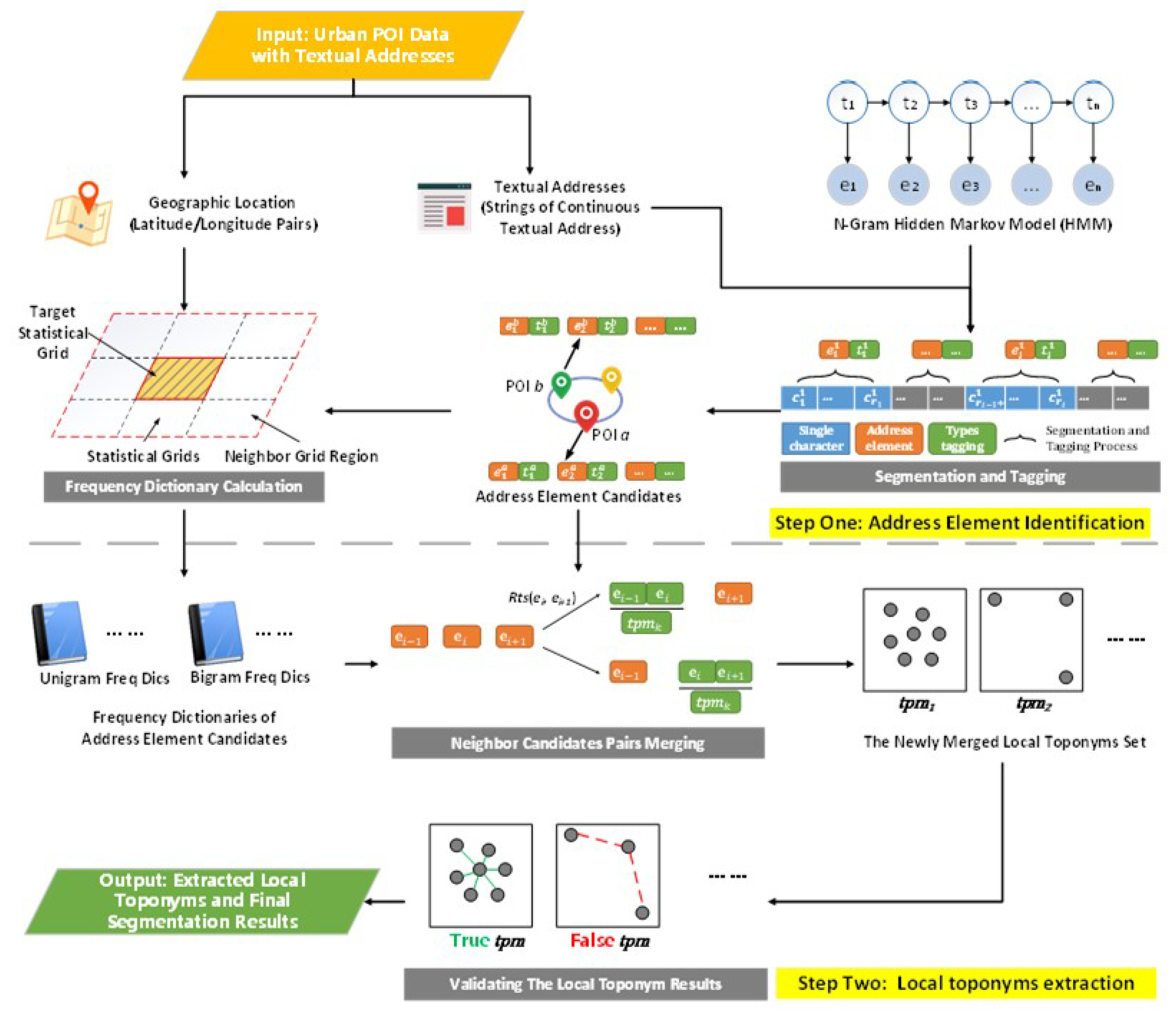
In this section, we propose a local spatial context-based framework to extract local toponyms and segment Chinese textual addresses from urban POI data. Proposed workflow for the proposed framework is illustrated in Figure 3. First, urban POIs with textual addresses are collected as an input data source; then, using the textual address and N-Gram hidden Markov model (HMM), address element candidates can be identified, and by using the local toponym spatial distribution patterns, the newly local toponyms set can be merged and true local toponyms can be validated and extracted. Finally, given these extracted true local toponyms, higher precision results of the textual address segmentation task can be achieved.

Figure 3.
The overall architecture of the proposed framework.
3.1. Input: Urban POI Data with Textual Addresses
One unique feature of the proposed framework is the use of urban POI data with textual addresses as an input raw-address corpus. Each urban POI with a textual address in the input dataset consists of three parts: a Chinese textual address, a geographic location, and other descriptive information. The first step of our framework examines the textual addresses of the POIs. The goal of the first step is to identify as many address element candidates as possible from a string of continuous textual addresses for each urban POI.
There are several advantages in using urban POI data with textual addresses as input data. First, the textual place detail information provided by urban POI data (including names, addresses, and other rich details) and the geospatial position coordinates gave a one-to-one correspondence, which meets our requirements for input data. Second, this type of data is available online and easily acquired. Many online digital map platforms such as Google Maps (https://www.google.com/maps/), Bing Maps (https://www.bing.com/maps), and Baidu Maps (https://map.baidu.com/ provide API services that support POI location data queries. Thus, our proposed framework can collect these data online (for example, by crawling urban POI data from digital map platforms) and apply our algorithms to the collected data. Moreover, the POI data provided by these platforms are constantly updated, so they can be used effectively to obtain updated address information over time.
3.2. Step One: Address Element Identification
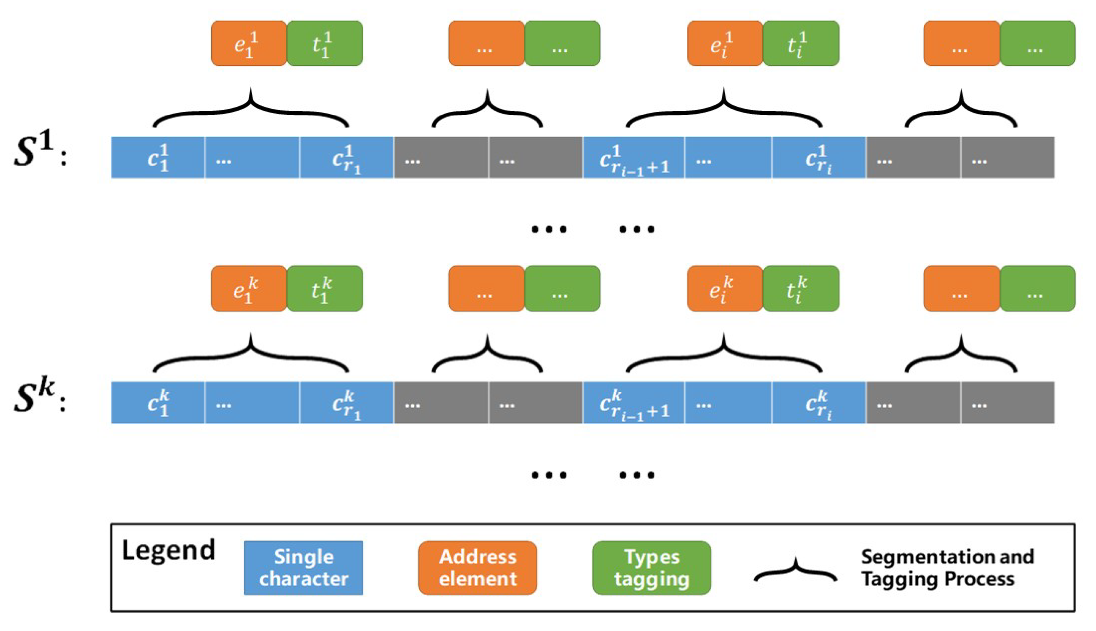
Considering that the Chinese address segmentation task involves identifying address elements and their types, it is similar to the NLP task of integrated word segmentation and syntactic type tagging, the goal of which is to identify individual words from a string of continuous sentence text in unsegmented languages, which do not have boundary markers between words. Figure 4 shows an example of identifying address elements from a string of continuous textual addresses, including administrative elements (e.g., Guangdong Province, Shenzhen City, Baoan District), local toponyms (e.g., Songrui Road), and house numbers (e.g., Number 350).

Figure 4.
An example of address elements identified from a continuous string of textual addresses.
In some NLP models, the processes of word segmentation and tagging are conducted in a step by step fashion, where word segmentation is applied first and word syntactic type tagging is applied afterward. However, making segmentation decisions without considering higher-level linguistic information, such as the syntactic types of the resulting words, maybe error-prone. A better approach is to keep all possible segmentations in a lattice form, score the lattice with a well-tagged syntactic type-based N-gram model, and finally, retrieve the best candidate using dynamic programming algorithms.
To identify the address element candidates from a string of continuous textual addresses, we construct an N-Gram hidden Markov model (HMM) to integrate the address segmentation and address element types tagging processes into one process. An HMM [38,39] is a finite state automaton with stochastic state transitions and observations. Based on the idea of HMM, the address element identification process can be considered as a decoding problem: given a model and an observation sequence (all possible segmentations of address element candidates in lattice form), determine the most likely states (address element types) that lead to the observation sequence. Let E represents a lattice of all possible segmentations of a given textual address A ( represents the i-th address element in the k-th segmentation Sk), T represent a lattice of address element type tags corresponding to E ( represents the address element type tag corresponding to ), and S = {s1, …, sk, …}w represents all possible segmentations with type tagging for the given textual address, as illustrated in Figure 5.
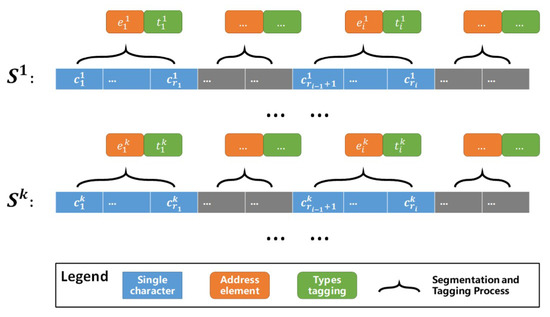
Figure 5.
The process of segmentation and address element type tagging from a string of continuous textual address.
The most likely segmentation and type tagging of a given textual address are computed by Equation (2):
where is a lattice of all possible segmentations of a given textual address , is a lattice of all segmented address element types tagging corresponding to . is a set of all possible segmentation results with types tagging for , is the k-th segmentation results of , is the i-th segmented address element in the k-th segmentation , and is the address element type tag corresponding to . is the transition probability between an adjacent pair of “hidden states” (address element types tagging) at positions i − 1 and i, and is the “emission probability” (conditional probability) of the observation variable given the probability of the hidden variable . All these probabilities are calculated based on a statistical frequency dictionary of address elements with types, which is well-trained before the segmentation and tagging process begins. Based on this equation, the Viterbi algorithm [40] is used to retrieve the best address element candidate sequence and its corresponding address element types.
Figure 6 shows an example of address element identification result using the N-Gram HMM model. As can be seen, administration units such as ‘深圳市’, ‘福田区’, local toponyms such as ‘深南中路’, and local numbers such as ‘4026号’, ‘16层’, ‘A’, are identified, while one local toponym ‘田面城市大厦’ is missed by this model and lead to a wrong segmentation result of this textual address. In the next step, we extracted these local toponyms based on their local spatial distribution characteristics to improve the precision of the final segmentation results.

Figure 6.
An example of address element identification using the N-Gram hidden Markov model (HMM) model.
With the prepared N-Gram HMM model, rough segmentation results can be calculated by applying the model to the original continuous textual addresses. In Section 4, we evaluate the performance of this model and compare it to our proposed model.
3.3. Step Two: Local Toponyms Extraction
Step one identifies address element candidates which also contain wrong address element candidate results (see Figure 6). This problem occurs because the performance of the N-Gram HMM model depends largely upon the coverage of the well-trained word frequency dictionary; however, using only the global statistical characteristics of corpus may ignore the spatial detail information of local toponyms distributed in only a small region (such as ‘田面城市大厦’ in Figure 6), which will lead to the out of vocabulary (OOV) problems when using the dictionary [5]. In turn, the OOV problems cause mis-extractions of many local toponyms in from the original textual addresses.
The main goal of step two is to merge neighboring address element candidate pairs into true local toponyms (such as merge ‘田面’ and ‘城市大厦’ into true local toponym ‘田面城市大厦’) and extract them to improve the final precision of the address segmentation task. Considering that the distribution of local toponyms is highly spatially related, different local toponyms will have certain spatial distribution patterns in different local regions. This characteristic can be used as supplementary information for local toponym extraction. In step two, we first explored the spatial distribution patterns of local toponyms; and then, we merged neighboring address element candidate pairs into local toponyms based on these patterns; finally, we validated the newly merged local toponym results by employing the geospatial cluster algorithm. The extraction step is accomplished through the following three sub-steps: 3.3.1 exploration of local toponym spatial distribution patterns, 3.3.2 merging neighboring candidate pairs, and 3.3.3 validating the local toponym results. Additional details are provided in the following subsections.
3.3.1. Exploration of Local Toponym Spatial Distribution Patterns
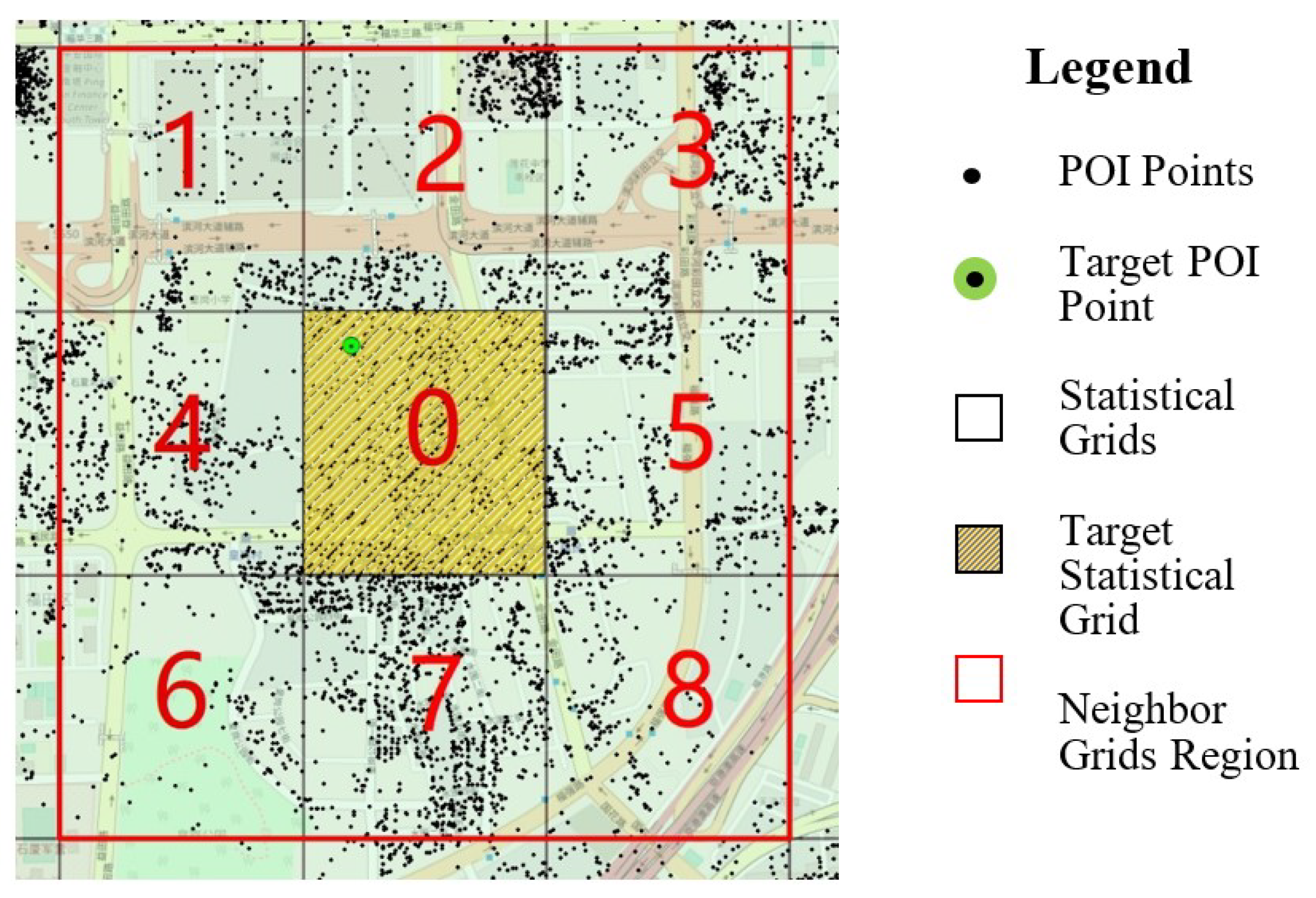
To explore the spatial distribution patterns of local toponyms, we divided the entire study area into a grid with 500 m cells and performed a spatial statistics on the corresponding rough segmentation results based on these grids. This spatial statistical analysis strategy is depicted in Figure 7.
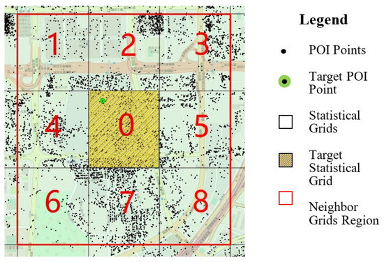
Figure 7.
The spatial statistical analysis strategy.
As shown in Figure 7, when we perform spatial statistical analysis on a target POI’s address rough segmentation results (newly identified address element candidates) within the target statistical grid (0.25 square km), all the POIs within a target statistical grid cell (cell 0) and all of the POIs within the eight-neighboring grid cells (cells 1–8, total area 2.25 square km) of the target statistical grid cell are involved in the spatial statistical analysis. Then, the unigram and bigram frequency dictionary of the address element candidates based on these POIs is calculated from the rough segmentation results for the target POI (see Algorithm 1 frequency dictionary calculation function). In the following, we briefly explain the procedure of Algorithm 1. Let sT (e1, e2, …, ei) represent the rough segmentation results of the target POI’s textual address, and let S^(s1, s2, …, sn) represent a set of the rough segmentation results of other POIs within the neighbor grids region (cells 1–8 in Figure 7). The main procedure of the uni-gram frequency dictionary calculation function is as follows: (1) Initialize uni-gram frequency dictionary D-1[str, count], in which ‘str’ is the uni-gram keyword and ‘count’ is the frequency of ‘str’; (2) for each address element candidate ei sT, we first append ei into D-1 with count = 1; (3) we iterate each rough segmentation results sj S^, and each address element candidate ek sj, if ek is the key of D-1, then we make the count of ek in D-1 plus one. Similar to the idea of the uni-gram frequency dictionary calculation function, the bigram frequency dictionary D-2 could be calculated by the bigram frequency dictionary calculation function, and then the statistical results D-1 and D-2 are used to calculate defined local spatial statistical variants to merge the address element candidates into new local toponyms.
| Algorithm 1:Frequency dictionary calculation | |
| Input: | |
| 1. The rough segmentation results of the target POI’s textual address is sT (e1, e2, …, ei), where ei is the address element candidate segmented from the textual address of the target POI; | |
| 2. The rough segmentation results of other POIs within the neighbor grids region is S^(s1, s2, …, sn). | |
| Output: The unigram and bigram frequency dictionaries, D-1 and D-2. | |
| def Uni-gram frequency dictionary calculation: | |
| Initialization: | |
| 1: | Initialize uni-gram frequency dictionary D-1[str, count], in which ‘str’ is the uni-gram keyword and ‘count’ is the frequency of ‘str’ |
| Iteration: | |
| 2: | for each address element candidate, ei sT do |
| 3: | D-1.append(ei, 1) |
| 4 | end for |
| 5: | for each rough segmentation results, sj S^ do |
| 6: | for each address element candidate, ek sj do |
| 7: | if ek is the key of D-1 |
| 8 | D-1[ek] += 1 |
| 9 | end if |
| 10: | end for |
| 11: | end for |
| 12: | returnD-1 |
| def Bigram frequency dictionary calculation: | |
| Initialization: | |
| 1: | Initialize bi-gram frequency dictionary D-2[str, count], in which ‘str’ is the bi-gram keyword and ‘count’ is the frequency of ‘str’ |
| Iteration: | |
| 2: | for each address element candidate, ei sT do |
| 3: | D-2.append(ei + ei+1, 1) |
| 4 | end for |
| 5: | for each rough segmentation results, sj S^ do |
| 6: | for each address element candidate, ek sj do |
| 7: | if (ek + ek+1) is_the_key of D-2 |
| 8 | D-2[ek + ek+1] += 1 |
| 9 | end if |
| 10: | end for |
| 11: | end for |
| 12: | returnD-2 |
Later, we performed a local spatial statistical analysis on the address element candidates for each target POI with local spatial statistical variants, including the conditional probability distribution p(ei+1| ei) and the information entropy H(ei), to measure the relatedness of the neighboring address element candidates in each target POI in the neighboring grid regions. Each region is small enough to explore the spatial distribution patterns of local toponyms. The statistical variants p(ei+1| ei) and H(ei) can be calculated by Equations (3) and (4).
In Equation (3), based on the “law of large numbers” theorem [41], p(ei, ei+1) is the co-occurrence probability of ei and ei+1, and p(ei) is the probability of ei in the neighboring grids, N is the total number of address element candidates for all POIs in the neighbor grids region, and freq(ei) and freq(ei, ei+1) can easily be found in the unigram and bigram frequency dictionaries, D-1 and D-2.
In Equation (4), ej is the next address element candidate after ei for a given POI, k is the total number of possible neighboring address element candidate pairs (ei and ej) when we assume that ei is the first item in these neighbor candidates pairs.
The statistical variants p(ei+1| ei) and H(ei) reflect how disorganized the neighbor candidate pairs are in a local region. We formulate these statistical variants into a model in the next subsection to measure the relatedness of neighbor address element candidate pairs.
3.3.2. Merging Neighbor Candidate Pairs
To determine which pairs of neighbor candidates should be merged into a new local toponym, we formulate the statistical variants freq(ei), p(ei+1| ei) and H(ei) into a new form Rts(ei, ei+1) to measure the relatedness of neighboring address element candidate pair (ei and ei+1) in the local neighboring grid cells using the following formula.
where exp() is an exponential function with a base natural constant of e. We use as the transform function for H(ei) for two reasons: (1) the value of H(ei) quantitatively reflects the disorder and uncertainty of the possible neighbor address element candidate pairs based on ei; the larger the value of H(ei) is, the less likely it is that ei will be a part of a new local toponym. Considering that g(x) is a monotonically decreasing and continuous function, g(H(ei)) will accurately reflect the changing trend of the relatedness of neighbor candidate pairs in a monotonically increasing form; (2) theoretically, the value of H(ei) ranges from 0 to +. After its transformation by g(x), the value of g(H(ei)) ranges from 0 to 1, thus the transformed variant g(H(ei)) could be used for the subsequent analysis more easily. The logarithm logb(freq(ei)) weakens the influence of freq(ei) and helps ensure that no single frequency of ei dominates the relatedness variant Rts(ei, ei+1). Here, b is a calibration parameter (we set b = 10 in this study). This logarithm adjustment was determined empirically; we also tested the freq(ei) approach.
After calculating the relatedness value, whether the neighboring candidates should be merged is determined by a threshold value, Rtsthrd. The strategy of neighbor candidates pairs merging is depicted in Figure 8 and by Algorithm 2, the merging neighboring candidate pairs function. Algorithm 2 shows the normal direction (from left to right, starting from the first address element candidates) of neighbor candidate pair-merging when calculating the relatedness value. We also tested other approaches, such as the reverse direction (from right to left, starting from the last address element candidates) and both directions (calculating the Rts values in both directions and choosing the larger result). Overall, which approach should be used as the final approach when calculating the relatedness value is determined empirically. We will present the empirical comparisons of these approaches in Section 4.

Figure 8.
The strategy for merging neighboring candidate pairs.
| Algorithm 2:Neighbor candidates pairs merging | |
| Input: | |
| 1. The rough segmentation results of the target POI, sT (e1, e2, …, ei), where ei is the address element candidate segmented from the textual address of the target POI; | |
| 2. The unigram and bigram frequency dictionaries, D-1 and D-2. | |
| Output: The newly merged local toponyms set, Tpm (tpm1, tpm2, …, tpmk). | |
| def Merging neighboring candidate pairs: | |
| Initialization: | |
| 1. | Initialize The newly merged local toponyms set Tpm [] |
| Iteration: | |
| 2. | for each address element candidate, ei sT do |
| 3. | Calculate Rts(ei−1, ei) based on Equation (5) |
| Calculate Rts(ei, ei+1) based on Equation (5) | |
| 4. | if Rts(ei−1, ei) > Rts(ei, ei+1) && Rts(ei−1, ei) > Rtsthrd |
| Merge ei−1 and ei into tpmk | |
| Tpm.append (tpmk) | |
| 5. | else If Rts(ei, ei+1) > Rts(ei−1, ei) && Rts(ei, ei+1) > Rtsthrd |
| Merge ei+1 and ei+1 into tpmk | |
| Tpm.append (tpmk) | |
| 6. | end if |
| 7. | end for |
| 8. | doAlgorithm 1 based on new Tpm [] |
| 9: | repeat steps 2–8 until no more updates to tpm occur |
| 10: | returnTpm [] |
3.3.3. Validating the Local Toponym Results
To validate the results of the extracted local toponyms, we employ the scale-structure identification (SSI) algorithm [30] to measure the geospatial cluster degree of the newly extracted local toponyms. This validation process is based on the intuitive assumption that the geospatial coordinates associated with a true local toponym are more likely to exhibit geospatial cluster; in contrast, the locations associated with a nonlocal toponym are more likely to be scattered around the entire local region [8]. The SSI algorithm attempts to cluster point coordinates at multiple geographic scales and examines their overall clustering degree. Therefore, the SSI algorithm can overcome the challenge that coordinates form different clusters at different scales under different distribution patterns, such as circle patterns and linear patterns.
Algorithm 3 shows the pseudocode for the local toponym clustering with SSI algorithm. The main mechanism of Algorithm 3 is as follows. (1) Let tpmk be a new extracted local toponym, and S-tpmk be a set of POI points whose textual address contains tpmk. Select POIs from the original urban POI dataset whose textual addresses contain tpmk, and add these POIs into S-tpmk. (2) Let R = { rm | m = 6, 7, 8, …, be an ordered set of distances that define the multiple clustering scales, where rm = am; a >1 (we use a = 2 m in this work); (3) Iterate m from 6 to M, and at each distance threshold, rm, let dij be the distance between Pti and Ptj in S-tpmk. Build an edge between Pti and Ptj if dij < rm, and add them into the same set of connected points, . (4) Calculate the entropy Em of all the connected point sets at scale m using Equation (6). (5) Calculate the final entropy value at all clustering scales, E-tpmk using Equation (7), and use E-tpmk as the clustering degree for the newly extracted local toponym, tpmk.
In Equation (6), Gm is the set of connected point sets under scale m, and represents a connected point set as a member of Gm. is the number of points in this set, and |S-tpmk| is the total number of points selected from the newly extracted local toponym tpmk.
In Equation (7), Em is the entropy of all the connected point sets at scale m, calculated using Equation (6). We set m from 6 to 11, which means that rm ranges from 64 to 2048 m—a distance range from 64 m to 2048 m is sufficient to perform geospatial clustering of POIs with the same local toponym. Here, p is a calibration parameter; we use p = 1, which was determined empirically. We also tested other approaches, including p = 1/|S-tpmk|, p = 1/log(|S-tpmk|) and p = 1/(|S-tpmk|)1/2. We will present these empirical comparisons in Section 4.
| Algorithm 3: Local toponym clustering with SSI | |
| Input: 1. The newly extracted local toponym, tpmk; 2. The original urban POIs dataset (UPD) with textual addresses. | |
| Output: The entropy value E-tpmk, which measures the geospatial clustering degree for tpmk. | |
| def Local toponym clustering: | |
| Initialization: | |
| 1: | Initialize a set of POI points whose textual address contains tpmk |
| 2: | Initialize a set of distances R = {rm | m = 6, 7, 8, …, M}, in which rm = am, a = 2 meters |
| SQL Query: | |
| 3: | Select POIs from UPD |
| where textual addresses of POIs | |
| contains tpmk | |
| 4: | S-tpmk.append(POIs) |
| Iteration: | |
| 5: | for each distance threshold rkR do |
| 6: | define a set of connected point sets Gm [ |
| 7: | for each pairwise points Pti, Ptj S-tpmk do |
| 8: | Calculate the pairwise distances dij between |
| Pti and Ptj | |
| 9: | if dij < rm |
| 10: | if Pti in |
| 11: | .append(Ptj) |
| 12: | else if Ptj in |
| 13: | .append(Pti) |
| 14: | else |
| 15: | initialize a new |
| 16: | .append(Pti) |
| 17: | .append(Ptj) |
| 18: | end if |
| 19: | end for |
| 20: | Calculate Em based on Equation (6) |
| 21: | end for |
| 22: | Calculate E-tpmk based on Equation (7) |
| 23: | returnE-tpmk |
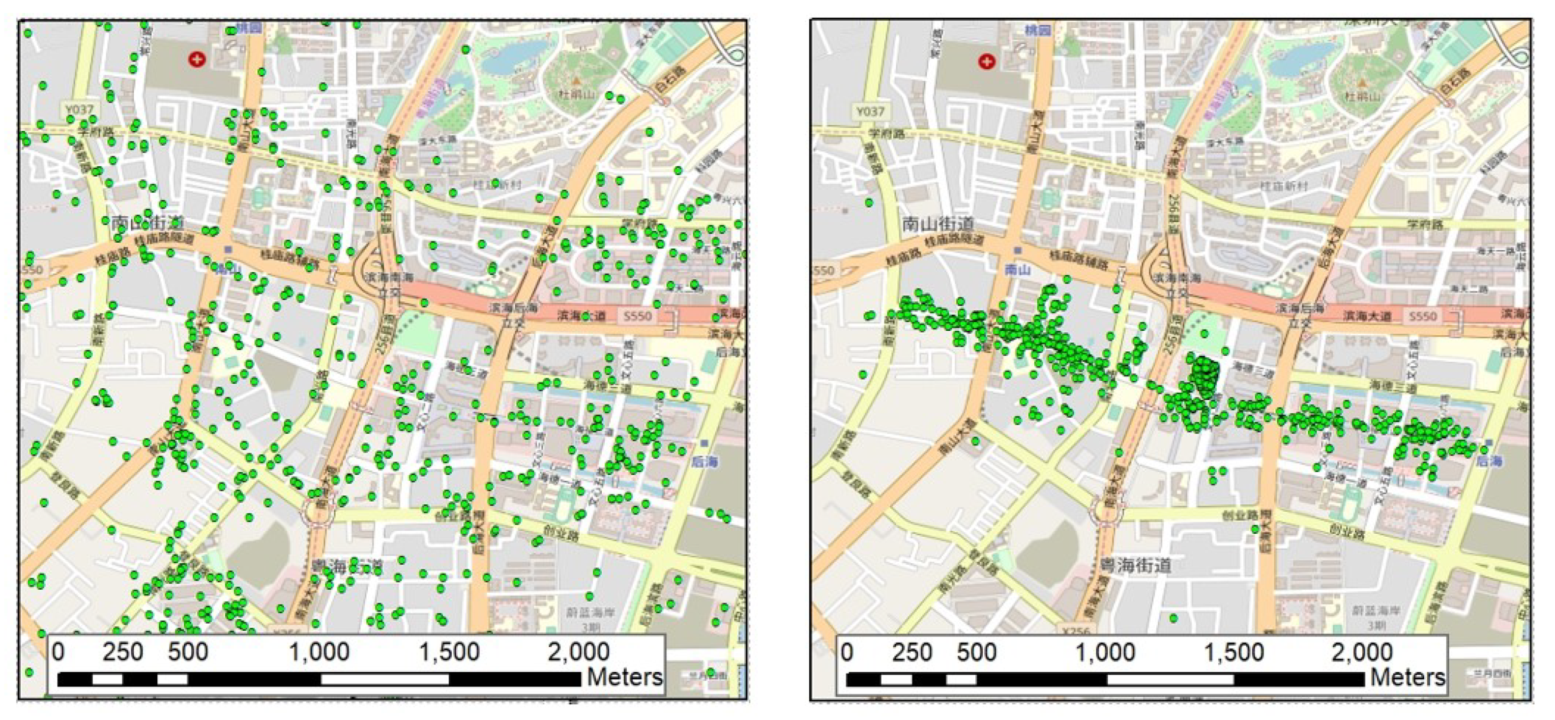
To obtain the final entropy value E-tpmk, tpmk is calculated at all clustering scales associated with the newly extracted local toponym candidate. Then, the geospatial clustering degree of tpmk is examined, and the results of the local toponym candidates extracted from the previous sub steps are validated. Finally, true local toponyms can be extracted based on E-tpmk. Figure 9 shows a point-distribution comparison between no local toponyms and true local toponyms. More details about the effect of E-tpmk in extracted local toponym result validation are presented in Section 4.
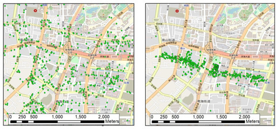
Figure 9.
A point-distribution comparison between no local toponyms (left) and true local toponyms (right) in the same area on the same scale.
3.4. Output: Extracted Local Toponyms and Final Segmentation Results
Step two extracts the local toponyms from the rough address segmentation results based on the spatial relatedness variants Rts(ei, ei+1) and the spatial clustering degree variant E-tpmk of the local toponym candidates in small local regions. The thresholds for Rts(ei, ei+1) and E-tpmk must be defined to merge neighboring candidate pairs and for results validation, respectively. These two thresholds can be determined based on precision-recall curves, which will be demonstrated in Section 4. Given these extracted true local toponyms, the address segmentation task results can be refined and achieve higher precision. We evaluate the performance of our model compared to those of previous traditional NLP models in Section 4.
4. Experiments
In this section, the proposed framework for an urban POI dataset is applied to extract local toponyms and segment textual addresses from Shenzhen City, China. We first describe the study areas and the dataset. Then, we present the results of multiple experiments. Finally, we provide an evaluation of the performance of the proposed framework.
4.1. Dataset
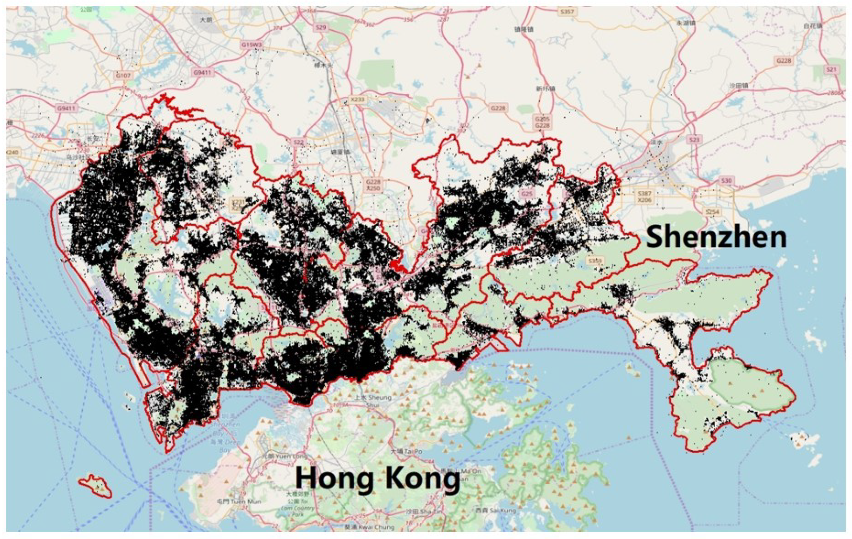
The experimental urban POI dataset was collected from the “open platform of Baidu Maps” (OPBM) (http://lbsyun.baidu.com/), which is the most popular online digital map platform in China. We selected Shenzhen City as the study area. Figure 10 presents an overview of the study area (the outlined red regions, with 10 subdistricts and an area of approximately 1996.78 km2). Shenzhen is located in Guangdong Province, China, which has experienced rapid growth over the past few decades and forms part of the Pearl River Delta megalopolis north of Hong Kong. In 2016, the permanent resident population in Shenzhen was 12 million, with a gross domestic product (GDP) of approximately 300 billion USD [42].
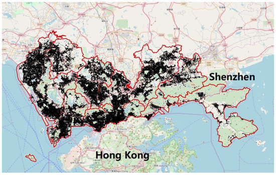
Figure 10.
Geographic distributions of the POIs in the study area, Shenzhen, China.
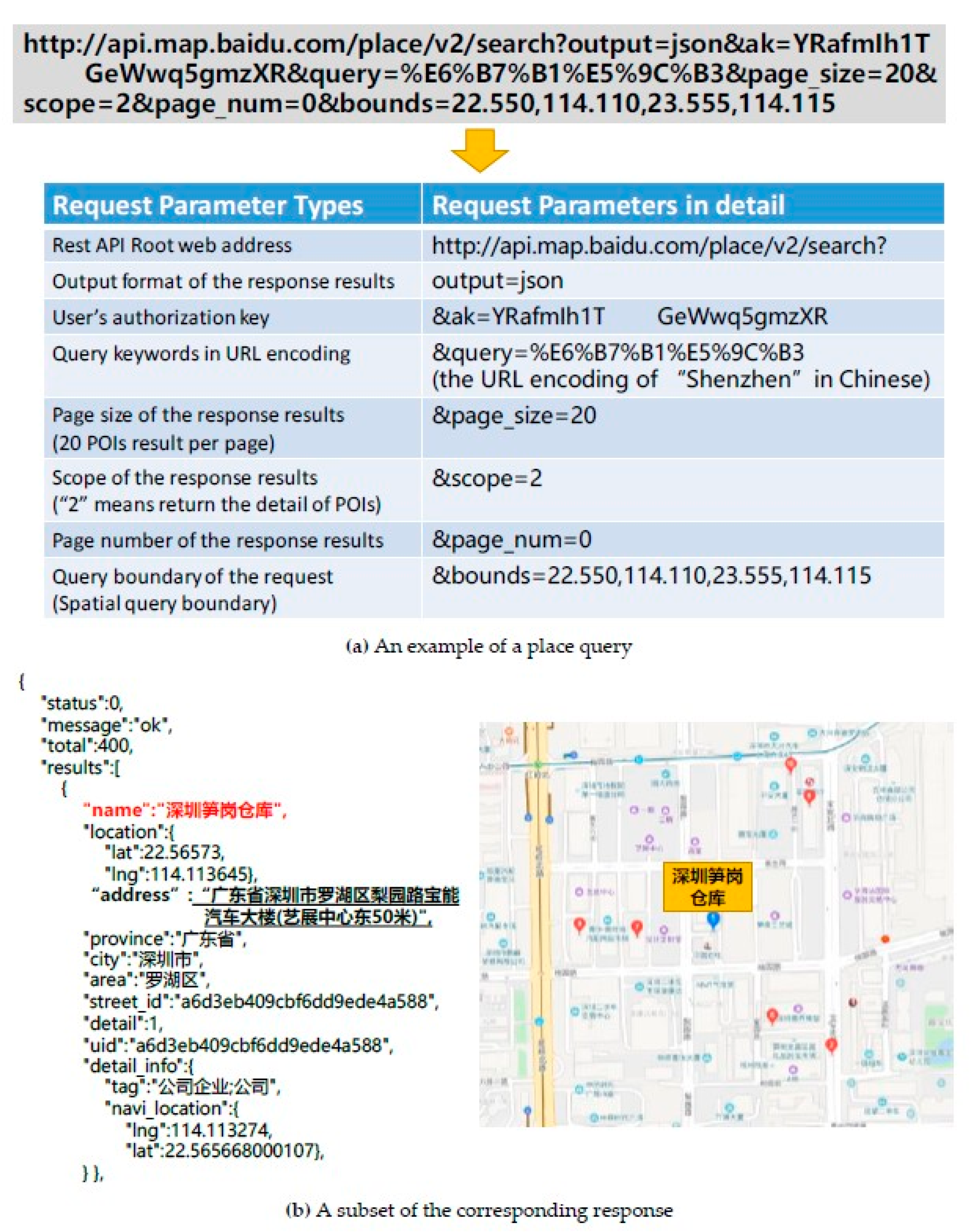
The urban POI dataset collection was accomplished by a web crawler written in C# (An object-oriented, advanced programming language that runs on top of the. NET Framework) and developed using the location API to retrieve POIs within the study area from the OPBM. Figure 11 shows an example of a location query and its response (retrieved POIs along with detail information are in JSON (JSON (JavaScript object notation) is a lightweight data exchange format) format). The requested URL constitutes a query to search for POIs within a certain geographic boundary related to the keyword “Shenzhen.” The corresponding response returns the POI results and associated detail information, including “name”, “location”, “address”, etc. in JSON format. Our web crawler parses these response results and extracts the textual addresses and the location information (longitude and latitude pairs) into the local database. In total, approximately 821,452 POIs were collected from the study area.
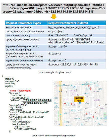
Figure 11.
An example of a place query and a subset of the corresponding response. (a) An example of a place query. (b) A subset of the corresponding response.
4.2. Experimental Designs
Using the collected urban POIs in the study area, the proposed N-Gram HMM model described in Section 3.2 is applied to the original textual addresses to retrieve the best address element candidate sequence and the corresponding address element types. These rough segmentation results are then combined with the spatial locations of the corresponding POIs. As the output of Step one, we obtain a set of rough segmented address element candidate sequences. Each address element sequence is associated with a point location. The performance of the N-Gram HMM model is evaluated and compared with traditional well-known NLP models in the next subsection. The algorithms of step one were implemented in Java programming language by using the Eclipse development IDE (A famous Java Integrated Development Environment (IDE), more details can be found at www.eclipse.org).
In Step Two, we first explore the spatial distribution patterns of the address element candidates based on their associated point locations; then, the relatedness of neighboring address element candidate pairs in the local region is measured to extract local toponyms. Finally, the results of the extracted local toponyms are validated using the SSI algorithm. All of the algorithms in step two were implemented in C# programming language by using Arc-Engine development tools (Arc-Engine 10.2, Environmental Systems Research Institute, Inc., more details can be found at www.esri.com).
After Step two, we can determine the thresholds for merging neighboring candidate pairs and for results validation, respectively, based on the precision-recall curves for extracting the candidates considered as true local toponyms. The process of determining the thresholds will be discussed in Section 4.3.
Using the extracted local toponyms, we can refine the rough address segmentation results in Step one to achieve higher precision. The final segmentation results of our proposed framework are evaluated and compared with other traditional NLP models (including our N-Gram HMM rough segmentation results) in Section 4.3.
4.3. Performance Evaluation
In this subsection, we evaluate the performance of our proposed framework. We first evaluate the performance of the proposed N-Gram HMM model and compare it with traditional well-known NLP models. Then, we discuss how to determine the thresholds for the spatial relatedness variant and the spatial clustering degree variant, respectively, based on precision-recall curves. Finally, we evaluate the performance of the final segmentation results of our proposed framework.
4.3.1. Ground-Truth Dataset Preparation
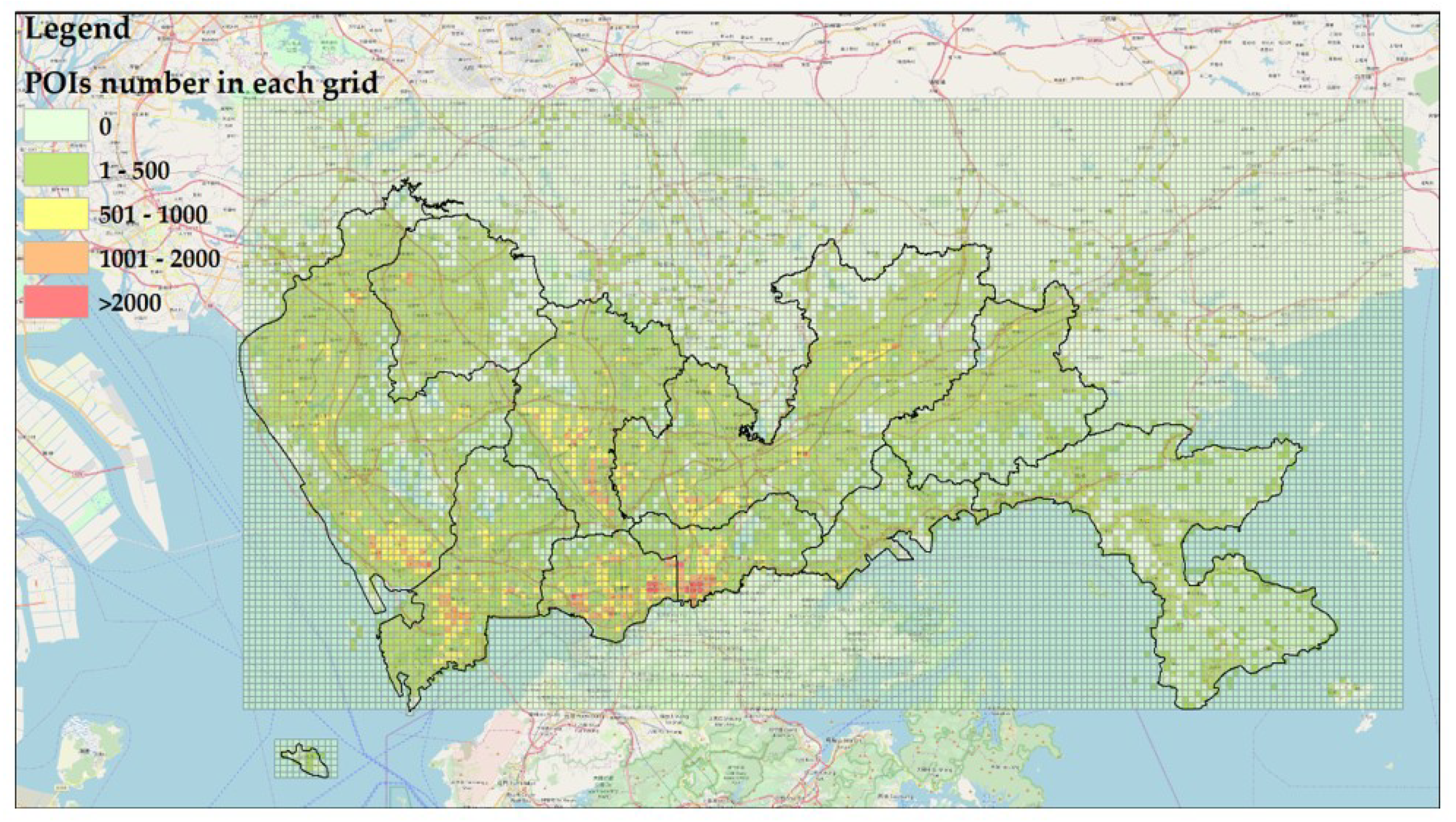
We start the evaluation by obtaining a well-segmented ground-truth dataset. Approximately 10,000 POIs with textual addresses randomly selected from the study area were manually segmented by a human parser. The POI selection strategy is based on the spatial distribution of POIs. We first divided the entire study area into grids with 500 m cell size and counted the number of POIs in each cell. Then, the number of POIs that should be selected from each grid was calculated based on Equation (8):
Nselected(gi) is the number of POIs that should be selected from grid-i, and Nselected(total) is the total number of POIs obtained for the ground-truth dataset. Here, Nselected(total) is 10,000, Ngi is the total number of POIs within grid-cell i and Ntotal is the total number of POIs within the whole study area. The POI distributions of each grid within the entire study area are shown in Figure 12.
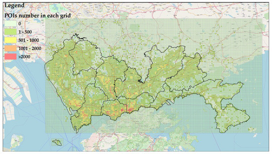
Figure 12.
The POI distributions of each grid in the entire study area.
After determining the number of POIs that should be selected from each grid, POIs with textual addresses were randomly selected from each grid and manually segmented into the ground-truth dataset for the subsequent evaluation experiments.
To quantify model performance, we employ the following three metrics from information retrieval, Precision (P), Recall (R) and F-score (F), which are respectively calculated as follows:
where NCS denotes the correct number of segmentation results, NS is the total number of segmentation results obtained using a model, and NO is the number of segmentation results in the original ground-truth dataset. Thus, Precision measures the percentage of correctly segmented results among all the segmented results returned by a model. Recall measures the percentage of correctly segmented results among all the segmented results that should be segmented (i.e., the ground-truth segmentation results obtained by a human parser), and F-score is the harmonic mean of precision and recall. The F-score is high when both precision and recall are high and it is low if either precision or recall is low.
4.3.2. Threshold Determination for Extracting Local Toponyms
Local toponym extraction is the key step in determining the final performance of the framework. The goal of this step is to merge neighboring address element candidates (identified in Step one) into local toponyms. Based on different thresholds for the spatial relatedness variant Rts(ei, ei+1) and the spatial clustering degree variant E-tpmk used to identify local toponym candidates in small local regions, different sets of local toponym candidates will be returned as the final output of Step two.
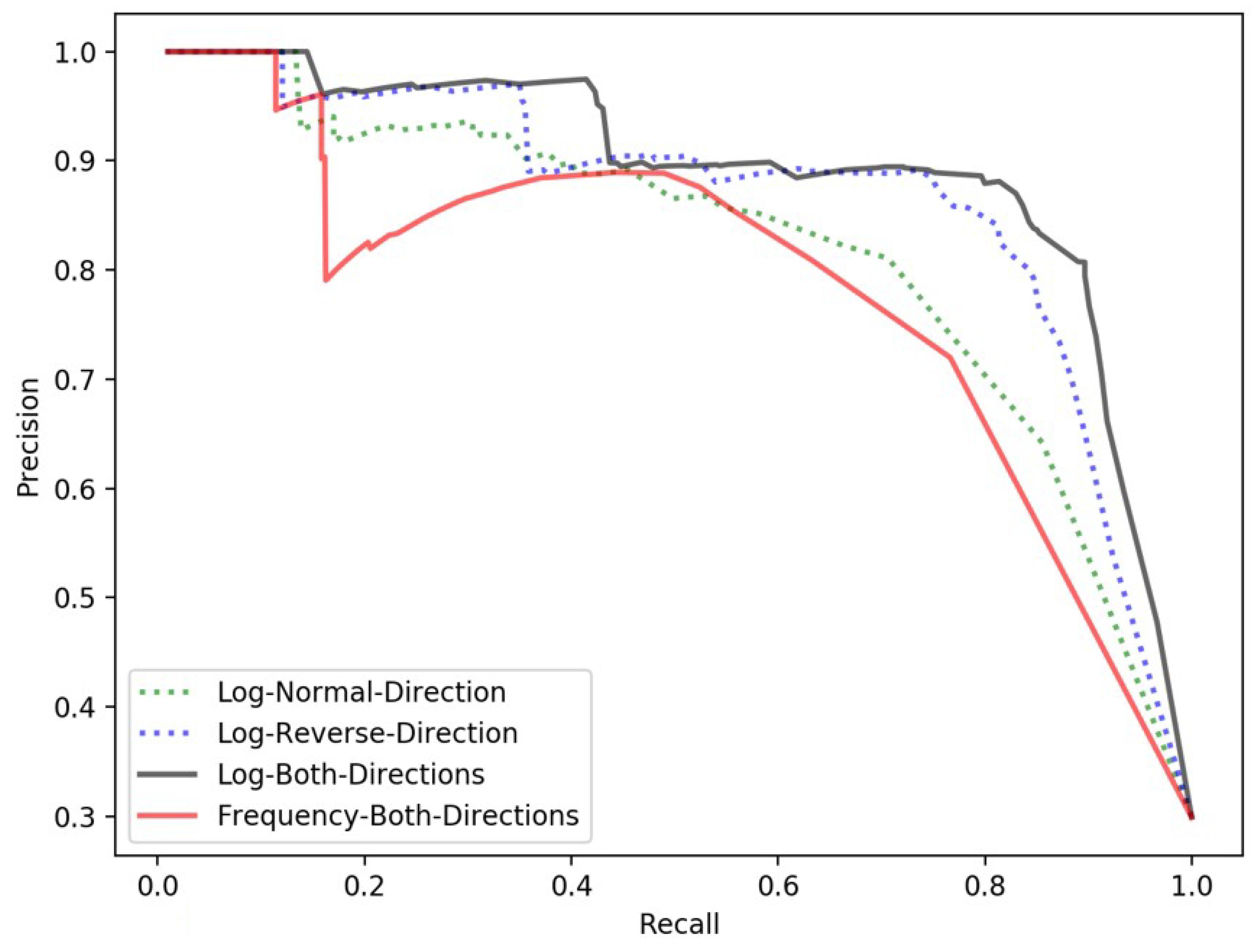
We normalize the spatial relatedness and spatial clustering degree variants to [0,1] based on their minimum and maximum values, respectively. Then, we iterate the threshold from 0 to 1 with a step size of 0.01. At each threshold, we obtain a precision, a recall, and an F-score. Using recall as the x coordinate and precision as the y coordinate, we can plot precision-recall curves to reveal the performances of Step two at the different thresholds. Figure 13 and Figure 14 show the precision-recall curves for the spatial relatedness and spatial clustering degree variants, respectively.

Figure 13.
The performances of proposed spatial relatedness models using different approaches and different adjustments.
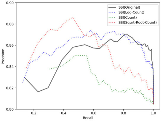
Figure 14.
The performances of the proposed spatial clustering degree model and other adjusted models.
To compare the proposed spatial relatedness models, we plot the precision-recall curves of the spatial relatedness obtained when using the forward direction, the reverse direction, and both directions. We also plot out the precision-recall curve of the spatial relatedness obtained with no logarithm adjustment using the both directions approach. We can evaluate the results of the different approaches and different adjustments by comparing the precision-recall curves. As shown in Figure 13, the spatial relatedness with logarithm adjustment using the both directions approach outperforms the other approaches in both precision and recall. Thus, we adopt this approach to calculate the spatial relatedness variant.
To compare the proposed spatial clustering degree model, we plot the precision-recall curves of the original SSI (without adjusting the entropy sums using the point counts, i.e., p = 1 in Equation (7)) along with three other possible ways of adjusting the entropy sums (i.e., point count, p = 1/|S-tpmk|, log point count, p = 1/log(|S-tpmk|) and square root point count p = 1/(|S-tpmk|)1/2 in Equation (7)). We can evaluate the proposed spatial clustering degree model by comparing its precision-recall curve with the performances of the other models. At first glance, all these curves achieve high precision, between 0.80 and 0.90. As the recall increases, the precision trends in each curve become complicated but are generally similar. When the recall is relatively low (under 0.60), the precision trends in each curve increase; and when the recall is relatively high (above 0.80), the precision trends in each curve decrease. In particular, the proposed spatial clustering degree model (original SSI) performs better than do the other adjusted models regarding both precision and recall when the recall is relatively high (above 0.80). This result suggests that when achieving the same precision, the proposed model correctly extracts more local toponyms than do the other three adjusted models. Thus, we adopted the original SSI approach to calculate the spatial clustering degree variant.
After determining the spatial relatedness and spatial clustering degree models, we calculated the corresponding thresholds for each model to extract the final local toponym results. These thresholds can be determined according to the needs of the application. Applications that require more correct output can use thresholds that produce high-precision (but lower recall). Conversely, applications that require higher coverage results can use thresholds with high recall (but low precision). For a balanced performance, one can choose the threshold with the highest F-score. Precision and recall are both important in this work, but we are inclined to lean toward precision because in the overall textual address segmentation task, precision is the more important performance indicator. Thus, we determine the threshold using the following steps: (1) we rank the thresholds based on their F-scores and identify those in the top 10; (2) among these 10 thresholds, we identify the one that results in the highest precision. The top-10 F-scores and the corresponding precision and recall scores for both the spatial relatedness and spatial clustering degree models are shown in Table 1 and Table 2. The selected final thresholds among these values are highlighted.

Table 1.
Top 10 F-scores for the spatial relatedness model.

Table 2.
Top 10 F-scores for the spatial clustering degree model.
Using this procedure, we selected a final threshold of 0.4989 for the spatial relatedness model, which yields a precision of 0.881, a recall of 0.814, and an F-score of 0.846. We selected a final threshold of 15.54627 for the spatial clustering degree model, which yields a precision of 0.856, a recall of 0.989, and an F-score of 0.918. After these thresholds have been determined, neighboring address element candidates can be merged into local toponym candidates. Approximately 605 different local toponym candidates were extracted (a precision of 0.856). Figure 15 shows the geographic distributions of some typical extracted local toponyms.
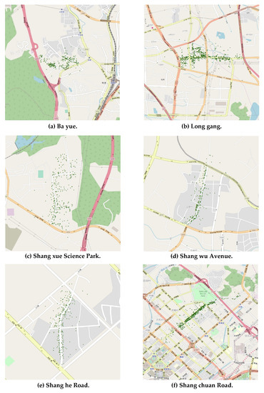
Figure 15.
Geographic distributions of typical extracted local toponyms.
4.3.3. Performance Evaluation of the Two-Step Framework
To evaluate the performance of the proposed framework, we conducted a set of textual address segmentation experiments on the ground-truth dataset. Three well-known Chinese word segmentation models and the step one proposed N-Gram HMM model were used in these experiments and compared with our two-step framework. The adopted three well-known Chinese word segmentation models for comparison are as follows:
- (a)
- jieba Word Segmenter (https://github.com/fxsjy/jieba);
- (b)
- HanLP Word Segmenter (https://github.com/hankcs/HanLP);
- (c)
- Stanford Word Segmenter (https://nlp.stanford.edu/software/segmenter.html).
Finally, we tested the performance of each model individually. As shown in Table 3, the step one proposed N-Gram HMM model achieves a precision of 0.812 and a recall of 0.893, much higher than the results of the other three tested Chinese word segmentation models. This result occurs because the N-Gram HMM model combines the address element segmentation and tagging process and retrieves the best candidate by calculating all the probabilities based on the statistical frequency dictionary of address elements with their types.

Table 3.
Performance of the proposed framework and other models.
We also compare the final performance of the two-step framework with using step one proposed N-Gram HMM model. Using the N-Gram HMM model, step one achieves a precision 0.812 and a relatively high recall 0.893. Adding step two increases the precision to 0.957 and also increases a recall to 0.945. This result occurs because the proposed framework extracts local toponyms by leveraging local spatial contextual information, which helps improve the precision of textual address segmentation for textual address data containing local toponyms. For example, the Chinese textual address shown in Figure 6, "深圳市福田区深南中路4026号田面城市大厦16层A”, contains the address element ‘田面城市大厦’, which is a local toponym located in a small local region. This toponym can easily be identified and extracted using our proposed framework.
5. Conclusions and Future Work
Segmenting and parsing textual addresses to extract local toponyms is a difficult but important task in the geocoding field, especially in China. This paper presents a local spatial context-based framework to extract local toponyms and segment Chinese textual addresses from urban POI data. First, an N-Gram HMM model is constructed to integrate address segmentation and tagging of address element types into a one-step process to identify the address element candidates from a string of continuous textual addresses. Then, the spatial distribution patterns of local toponyms in different local regions are explored. Based on these patterns, we apply a series of spatial statistical approaches to quantify the spatial relatedness and the spatial clustering degree of the local toponyms. Two thresholds can then be determined to extract the true local toponyms. We applied the proposed framework to a ground-truth POI dataset collected in Shenzhen City, China to extract local toponyms and segment textual addresses and evaluated the performance of our model in terms of precision, recall, and F-score. We compared the segmentation results of the proposed framework with three well-known Chinese word segmentation models, jieba, HanLP, and Stanford, to demonstrate the outstanding performance of the proposed framework.
The contributions of this paper can be seen from three perspectives. From a data source perspective, this paper uses automatically collected urban POI data as input data, in which the textual addresses and the geospatial position coordinates have a one-to-one correspondence and can be easily used to explore the spatial distribution of local toponyms. From a methodology perspective, this work involves local spatial distribution patterns and formulates spatial statistical parameters (i.e., spatial relatedness and spatial clustering degree to effectively extract local toponyms in small local regions. The methods illustrated in this paper are generic and can be applied directly to other Chinese textual address datasets. From an application perspective, this paper presents a computational framework that combines the traditional NLP and spatial statistical analysis approaches. As indicated by the experimental results, the integrated framework achieves outstanding performance when extracting local toponyms and segmenting textual addresses, easily outperforming the well-known NLP model, which is based on linguistic features alone.
Although the proposed framework achieves good results for local toponym extraction and textual address segmentation, some future work is still required. First, the proposed framework is based on a series of spatial analysis algorithms that are often time-consuming; thus, the efficiency of the entire framework should be optimized. Second, the final result of the framework (i.e., The well-segmented address elements and local toponyms) are still disorganized. Further studies can be conducted on how to automatically store these address elements and local toponyms into digital gazetteers.
Author Contributions
Conceptualization, Renzhong Guo and Biao He; data curation, Xi Kuai; formal analysis, Biao He; funding acquisition, Biao He; investigation, Zhigang Zhao; methodology, Xi Kuai; project administration, Biao He; resources, Zhijun Zhang; software, Zhijun Zhang and Zhigang Zhao; supervision, Renzhong Guo and Biao He; validation, Xi Kuai and Han Guo; visualization, Han Guo; writing—original draft, Xi Kuai. All authors have read and agreed to the published version of the manuscript.
Funding
This research was funded by the Open Fund of Key Laboratory of Urban Land Resources Monitoring and Simulation, Ministry of Land and Resources, Shenzhen, PR China, grant number: KF-2018-03-009 and supported by National Natural Science Foundation of China, grant number: 41901325.
Acknowledgments
The authors would like to thank Gang Luo, the author of the book “Principles and techniques of natural language processing, Electronic Industry Press”, and this book inspired the design of the main methodology of this article. We are grateful for helpful comments from the journal editors and three anonymous reviewers.
Conflicts of Interest
The authors declare no conflict of interest.
References
- Roongpiboonsopit, D.; Karimi, H.A. Comparative evaluation and analysis of online geocoding services. Int. J. Geogr. Inf. Sci. 2010, 24, 1081–1100. [Google Scholar] [CrossRef]
- Hill, L.L. Georeferencing: The Geographic Associations of Information; MIT Press: Cambridge, MA, USA; London, UK, 2009. [Google Scholar]
- Zhu, R.; Hu, Y.; Janowicz, K.; McKenzie, G. Spatial signatures for geographic feature types: Examining gazetteer ontologies using spatial statistics. Trans. GIS 2016, 20, 333–355. [Google Scholar] [CrossRef]
- Goldberg, D.W. Advances in Geocoding Research and Practice. Trans. GIS 2011, 15, 727–733. [Google Scholar] [CrossRef]
- Li, L.; Wang, W.; He, B.; Zhang, Y. A hybrid method for Chinese address segmentation. Int. J. Geogr. Inf. Sci. 2017, 32, 30–48. [Google Scholar] [CrossRef]
- Oshikiri, T. Segmentation-Free Word Embedding for Unsegmented Languages. In Proceedings of the 2017 Conference on Empirical Methods in Natural Language Processing, Copenhagen, Denmark, 7–11 September 2017. [Google Scholar]
- Chowdhury, G.G. Natural language processing. Annu. Rev. Inf. Sci. Technol. 2003, 37, 51–89. [Google Scholar] [CrossRef]
- Hu, Y.; Mao, H.; McKenzie, G. A natural language processing and geospatial clustering framework for harvesting local place names from geotagged housing advertisements. Int. J. Geogr. Inf. Sci. 2018, 33, 714–738. [Google Scholar] [CrossRef]
- Kuo, C.-L.; Chan, T.-C.; Fan, I.-C.; Zipf, A. Efficient Method for POI/ROI Discovery Using Flickr Geotagged Photos. ISPRS Int. J. Geo-Inf. 2018, 7, 121. [Google Scholar] [CrossRef]
- GB/T 23705-2009: The Rules of Coding for Address in the Common Platform for Geospatial Information Service of Digital City; Standards Press of China: Beijing, China, 2009.
- W3C. Points of Interest. 2010. Available online: https://www.w3.org/2010/POI/wiki/Main_Page (accessed on 19 November 2019).
- Zhang, M.; Yu, N.; Fu, G. A Simple and Effective Neural Model for Joint Word Segmentation and POS Tagging. IEEE/ACM Trans. Audio Speech Lang. Process. 2018, 26, 1528–1538. [Google Scholar] [CrossRef]
- Kamper, H.; Jansen, A.; Goldwater, S. Unsupervised Word Segmentation and Lexicon Discovery Using Acoustic Word Embeddings. IEEE/ACM Trans. Audio Speech Lang. Process. 2016, 24, 669–679. [Google Scholar] [CrossRef]
- Eler, D.M.; Grosa, D.F.P.; Pola, I.; Garcia, R.; Correia, R.C.M.; Teixeira, J. Analysis of Document Pre-Processing Effects in Text and Opinion Mining. Information 2018, 9, 100. [Google Scholar] [CrossRef]
- Magistry, P.; Sagot, B. Unsupervized word segmentation: The case for Mandarin Chinese. In Proceedings of the 50th Annual Meeting of the Association for Computational Linguistics: Short Papers; Association for Computational Linguistics: Stroudsburg, PA, USA, 2012. [Google Scholar]
- Kang, M.; Du, Q.; Wang, M. A New Method of Chinese Address Extraction Based on Address Tree Model. Acta Geod. Cartogr. Sin. 2015, 44, 99–107. [Google Scholar]
- Tian, Q.; Ren, F.; Hu, T.; Liu, J.; Li, R.; Du, Q. Using an Optimized Chinese Address Matching Method to Develop a Geocoding Service: A Case Study of Shenzhen, China. ISPRS Int. J. Geo-Inf. 2016, 5, 65. [Google Scholar] [CrossRef]
- Zhou, H.; Du, Z.; Fan, R.; Ma, L.; Liang, R. Address model based on spatial-relation and Its analysis of expression patterns. Eng. Surv. Mapp. 2016, 5, 25–31. [Google Scholar]
- Mochihashi, D.; Yamada, T.; Ueda, N. Bayesian unsupervised word segmentation with nested Pitman-Yor language modeling. In Proceedings of the Joint Conference of the 47th Annual Meeting of the ACL and the 4th International Joint Conference on Natural Language; Association for Computational Linguistics: Stroudsburg, PA, USA, 2009; pp. 100–108. [Google Scholar]
- Zhikov, V.; Takamura, H.; Okumura, M. An Efficient Algorithm for Unsupervised Word Segmentation with Branching Entropy and MDL. Trans. Jpn. Soc. Artif. Intell. 2013, 28, 347–360. [Google Scholar] [CrossRef]
- Huang, L.; Du, Y.; Chen, G. GeoSegmenter: A statistically learned Chinese word segmenter for the geoscience domain. Comput. Geosci. 2015, 76, 11–17. [Google Scholar] [CrossRef]
- Yan, Y.; Kuo, C.-L.; Feng, C.-C.; Huang, W.; Fan, H.; Zipf, A. Coupling maximum entropy modeling with geotagged social media data to determine the geographic distribution of tourists. Int. J. Geogr. Inf. Sci. 2018, 32, 1699–1736. [Google Scholar] [CrossRef]
- Huang, Z.; Xu, W.; Yu, K. Bidirectional LSTM-CRF models for sequence tagging. arXiv 2015, arXiv:1508.01991. [Google Scholar]
- Cai, D.; Zhao, H. Neural word segmentation learning for Chinese. arXiv 2016, arXiv:1606.04300. [Google Scholar]
- Ma, X.; Hovy, E. End-to-end Sequence Labeling via Bi-directional LSTM-CNNs-CRF. In Proceedings of the 54th Annual Meeting of the Association for Computational Linguistics (Volume 1: Long Papers); Association for Computational Linguistics: Berlin, Germany, 2016. [Google Scholar]
- Zhang, M.; Zhang, Y.; Fu, G. Transition-based neural word segmentation. In Proceedings of the 54th Annual Meeting of the Association for Computational Linguistics (Volume 1: Long Papers); Association for Computational Linguistics: Berlin, Germany, 2016. [Google Scholar]
- Zhang, Y.; Li, C.; Barzilay, R.; Darwish, K. Randomized greedy inference for joint segmentation, POS tagging and dependency parsing. In Proceedings of the 2015 Conference of the North American Chapter of the Association for Computational Linguistics: Human Language Technologies; Association for Computational Linguistics: Denver, CO, USA, 2015. [Google Scholar]
- Kurita, S.; Kawahara, D.; Kurohashi, S. Neural joint model for transition-based Chinese syntactic analysis. In Proceedings of the 55th Annual Meeting of the Association for Computational Linguistics (Volume 1: Long Papers); Association for Computational Linguistics: Vancouver, BC, Canada, 2017. [Google Scholar]
- Hu, Y.; Janowicz, K. An empirical study on the names of points of interest and their changes with geographic distance. arXiv 2018, arXiv:1806.08040. [Google Scholar]
- Rattenbury, T.; Good, N.; Naaman, M. Towards automatic extraction of event and place semantics from flickr tags. In Proceedings of the 30th Annual International ACM SIGIR Conference on Research and Development in Information Retrieval, Amsterdam, The Netherlands, 23–27 July 2007. [Google Scholar]
- Katragadda, S.; Chen, J.; Abbady, S. Spatial hotspot detection using polygon propagation. Int. J. Digit. Earth 2018, 12, 825–842. [Google Scholar] [CrossRef]
- Li, D.; Wang, S.; Li, D. Spatial Data Mining; Springer: Berlin/Heidelberg, Germany, 2015. [Google Scholar]
- Mai, G.; Janowicz, K.; Hu, Y.; Gao, S. ADCN: An anisotropic density-based clustering algorithm for discovering spatial point patterns with noise. Trans. GIS 2018, 22, 348–369. [Google Scholar] [CrossRef]
- Birant, D.; Kut, A. ST-DBSCAN: An algorithm for clustering spatial–temporal data. Data Knowl. Eng. 2007, 60, 208–221. [Google Scholar] [CrossRef]
- Kisilevich, S.; Mansmann, F.; Keim, D. P-DBSCAN: A density based clustering algorithm for exploration and analysis of attractive areas using collections of geo-tagged photos. In Proceedings of the 1st International Conference and Exhibition on Computing for Geospatial Research & Application, Washington, DC, USA, 21–23 June 2010. [Google Scholar]
- Ruiz, C.; Spiliopoulou, M.; Menasalvas, E. C-dbscan: Density-Based Clustering with Constraints. In International Workshop on Rough Sets, Fuzzy Sets, Data Mining, and Granular-Soft Computing; Springer: Toronto, QC, Canada, 2007. [Google Scholar]
- Du, Q.; Dong, Z.; Huang, C.; Ren, F. Density-Based Clustering with Geographical Background Constraints Using a Semantic Expression Model. ISPRS Int. J. Geo-Inf. 2016, 5, 72. [Google Scholar] [CrossRef]
- Rabiner, L. A tutorial on hidden Markov models and selected applications in speech recognition. Proc. IEEE 1989, 77, 257–286. [Google Scholar] [CrossRef]
- Law, H.H.-C.; Chan, C. Ergodic multigram HMM integrating word segmentation and classtagging for Chinese language modeling. In Proceedings of the IEEE International Conference on Acoustics, Speech, and Signal Processing Conference Proceedings, Atlanta, GA, USA, 9 May 1996. [Google Scholar]
- Forney, G. The viterbi algorithm. Proc. IEEE 1973, 61, 268–278. [Google Scholar] [CrossRef]
- Cthaeh. The Law of Large Numbers: Intuitive Introduction. 2018. Available online: https://www.probabilisticworld.com/law-large-numbers/ (accessed on 27 November 2019).
- Wang, S.; Xu, G.; Guo, Q. Street Centralities and Land Use Intensities Based on Points of Interest (POI) in Shenzhen, China. ISPRS Int. J. Geo-Inf. 2018, 7, 425. [Google Scholar] [CrossRef]
© 2020 by the authors. Licensee MDPI, Basel, Switzerland. This article is an open access article distributed under the terms and conditions of the Creative Commons Attribution (CC BY) license (http://creativecommons.org/licenses/by/4.0/).

