1. Introduction
A well-developed public transport system is the key to achieving citizens’ mobility in an environmentally sustainable fashion. Due to demand fluctuations and traffic congestion, it is a challenging task for operators to ensure the efficiency of public transport service and improve travel time reliability [
1]. Unreliable service causes passengers to require extra travel time due to the headway irregularity of buses, and imposes additional costs on operators because of the ineffective utilization of allocated resources. Therefore, there is a growing realization that the alleviation of traffic congestion through public transport network (PTN) optimization is a fundamental solution to reduce high traffic congestion costs, lower energy consumption, lessen air pollution, and improve mobility [
2].
Most of the previous PTN optimization models were formulated as bi-level problems whose objectives are to minimize both the operators’ and users’ costs [
3]. In-vehicle travel time, stop spacing, frequency of service, capacity, and congestion related to over-crowded vehicles are usually considered as variables in network optimization problems. Examples of these models can be seen in the studies of References [
4,
5,
6]. Due to the NP(non-deterministic polynomial)-hard nature of optimizing all the variables simultaneously, metaheuristic approaches that pursue worthy local optimal results are proposed. For example, Mesbah et al. [
7] proposed a bi-level approach to optimize the transport road space priority for a road network using the parallel genetic algorithm. However, these network optimization models developed in the above-mentioned articles had been usually applied in uncongested road segments.
Public traffic condition refers to the traffic volume of the road network and its dynamic spatial-temporal distribution, which can reflect the degree of congestion [
8]. Recently, the traffic congestion impacts of bus operations on a road segment or a corridor have been investigated by researchers [
9,
10]. These congestion effects mainly include the effects of bus stop design, bus travel time, and bus priority options such as exclusive bus lanes or priority signals for buses [
9]. Understanding these congestion impacts can help operators to identify the effectiveness of transport network optimization in relieving congested areas or congested routes. For example, under congested traffic conditions, it is difficult for buses to return to the driving lane, which leads to a longer travel time after picking-up/dropping off passengers at stops [
11]. Furthermore, the bus travel time variation dominated by traffic congestion often results in unreliable service, which has negative impacts on both the operators and passengers [
12]. Previous studies have pointed out that well-located stops have the potential to alleviate the impact of traffic congestion [
3]. Therefore, it is critical to optimize PTN by considering the impact of traffic congestion in order to achieve a high level of public transport service and improve travel time reliability.
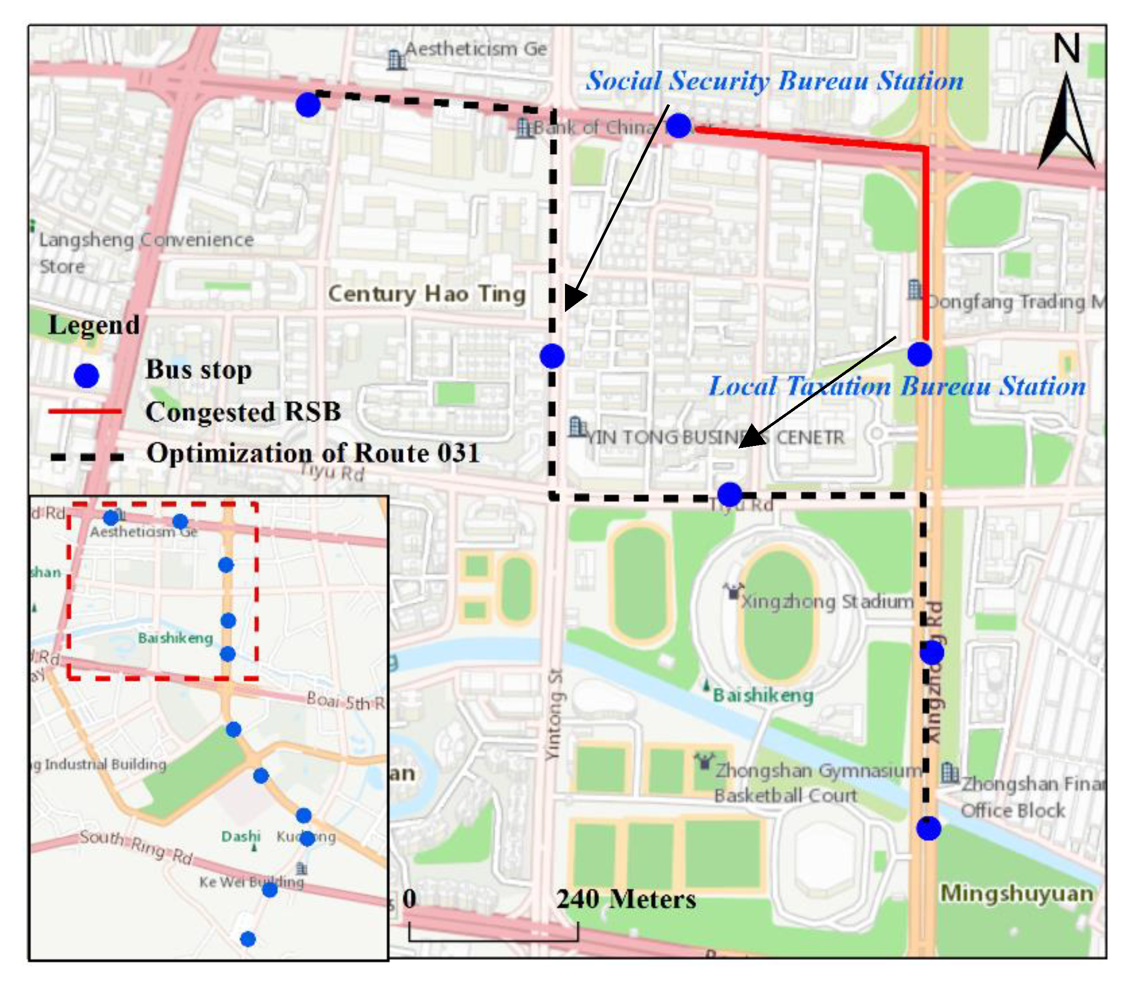
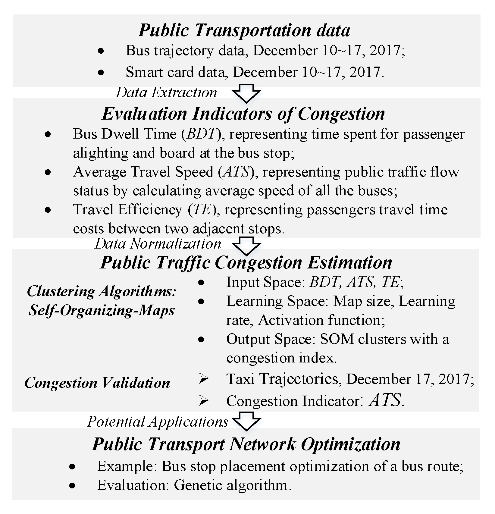
In this study, we proposed a data-based methodology to estimate the traffic congestion of road segments between bus stops (RSBs) using a self-organizing feature map (SOM). The SOM was used to cluster and effectively recognize traffic patterns embedded in the RSBs. Furthermore, a congestion index for ranking the SOM clusters was developed to determine the congested RSBs. Based on the congested RSBs, an exploratory example of PTN optimization was discussed and evaluated using a genetic algorithm. The main contributions of this study were summarized as follows:
(1) Public traffic congestion estimation: We estimated the traffic congestion of the RSBs using SOM based on bus trajectory data and smart card data. In contrast to the traditional methods using taxi trajectory data, our methodology could be applied to estimate the congested RSBs with bus priority lanes or with limited taxi trips, which can benefit various applications including road traffic status estimation, PTN optimization, and urban transport system management.
(2) PTN optimization considering traffic congestion: Based on the congested RSBs, an exploratory example of PTN optimization was discussed and evaluated using a genetic algorithm. The empirical results contributed to the development of more efficient strategies for PTN optimization by considering public traffic congestion.
The rest of this paper is organized in the following way. The next section provides a literature review.
Section 3 describes our proposed methodology, followed by a case study in
Section 4. The discussion of the strategies for PTN optimization is provided in
Section 5. Finally, we briefly conclude in
Section 6 with limitations and future research directions.
Figure 1 presents the research framework.
3. Methodology
In this section, we describe the proposed methodology in detail and give the definitions for the entire paper to avoid possible confusion. A comprehensive analysis of PTN requires the consideration of multiple travel times, including the passengers’ boarding/alighting time and bus dwell time at bus stops. Therefore, this study exploits several important properties about the traffic condition of the RSBs and builds a reliability-based methodology to estimate public traffic congestion.
3.1. Definitions
To make a clear statement of the bus routes and their characteristics, we will clarify some basic definitions, including the bus line, bus trajectory data, bus dwell time, average travel speed, and travel efficiency.
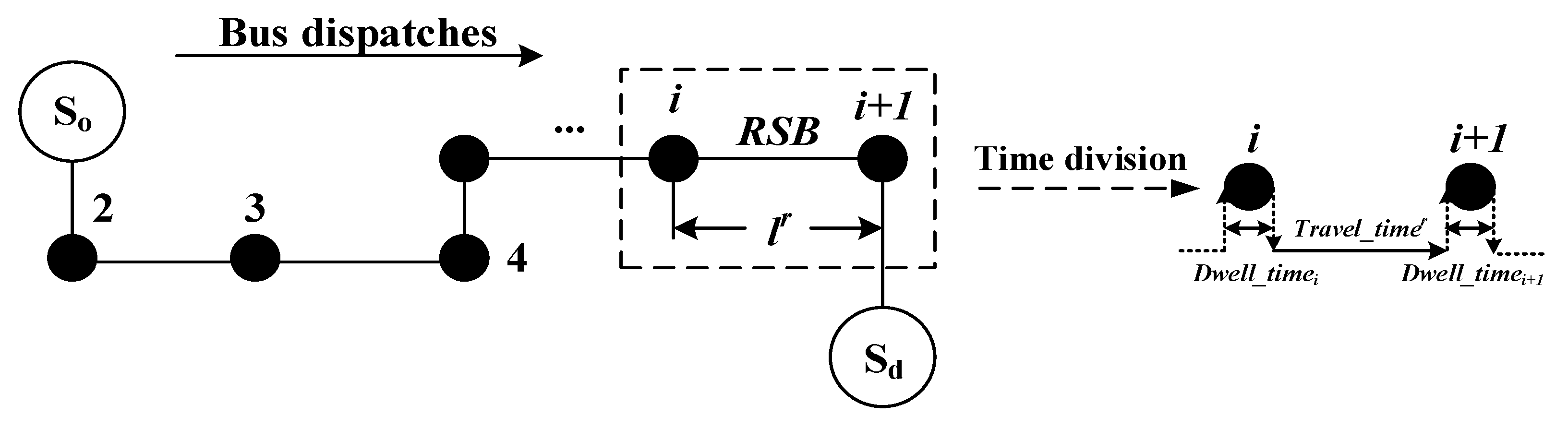
Definition 1. Bus Line:we consider a general bus line of length L that consists of n bus stops, which is shown in Figure 2. where
So, Sd – Terminal bus stops of a bus line.
RSB – One road segment between adjacent bus stops of a bus line.
i – The index of the bus stops.
– Length of RSB r.
Definition 2. Bus Trajectory Data:Bus trajectory data is a dataset that describes bus movements, including the location points in a time sequence: idi, xi, yi, ti, spei, diri, while 1≤i<k, idi is a unique code for a bus, ti is a time-stamp, (xi, yi) are the latitude and longitude coordinates, spei is the bus speed and diri is the moving direction.
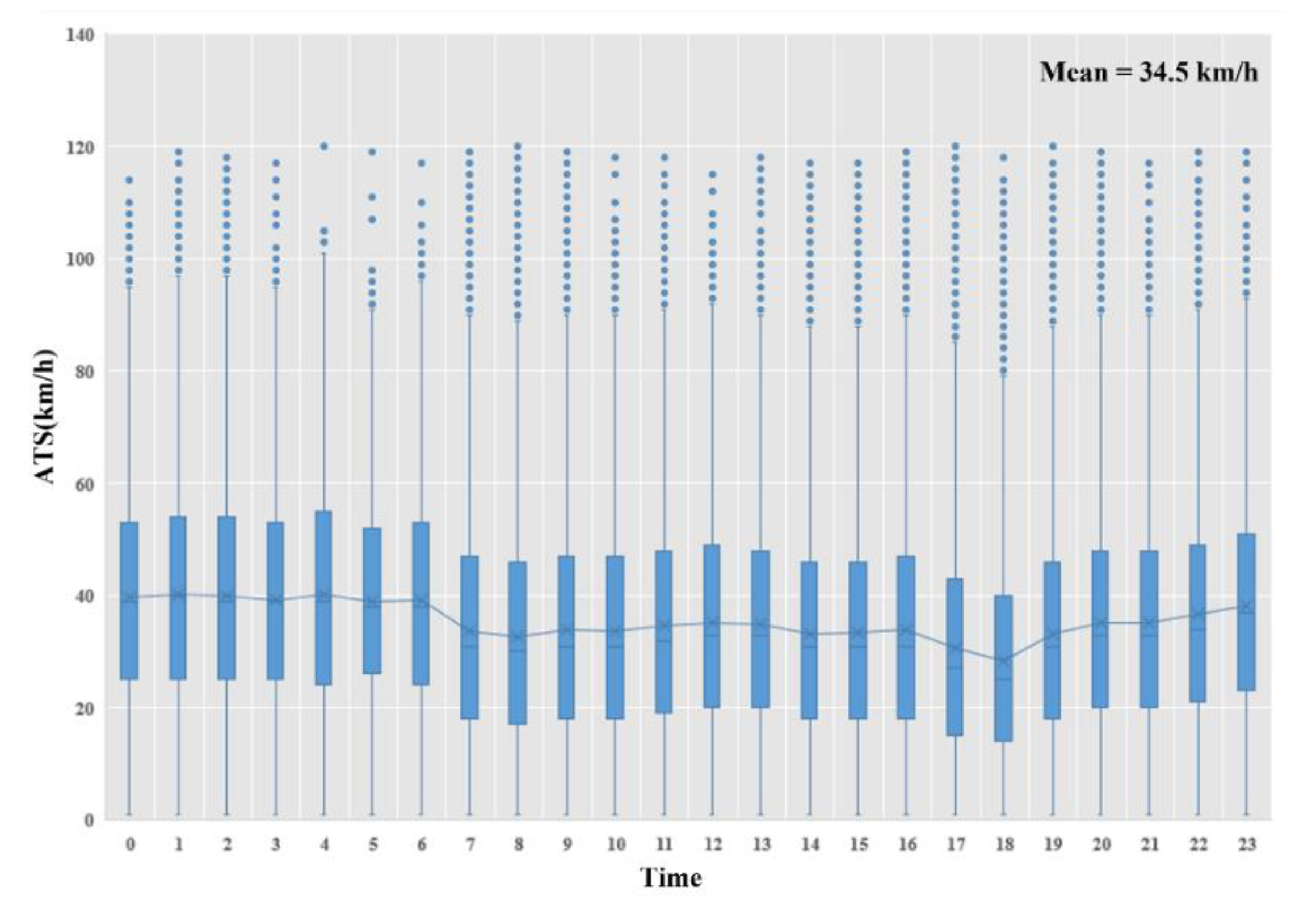
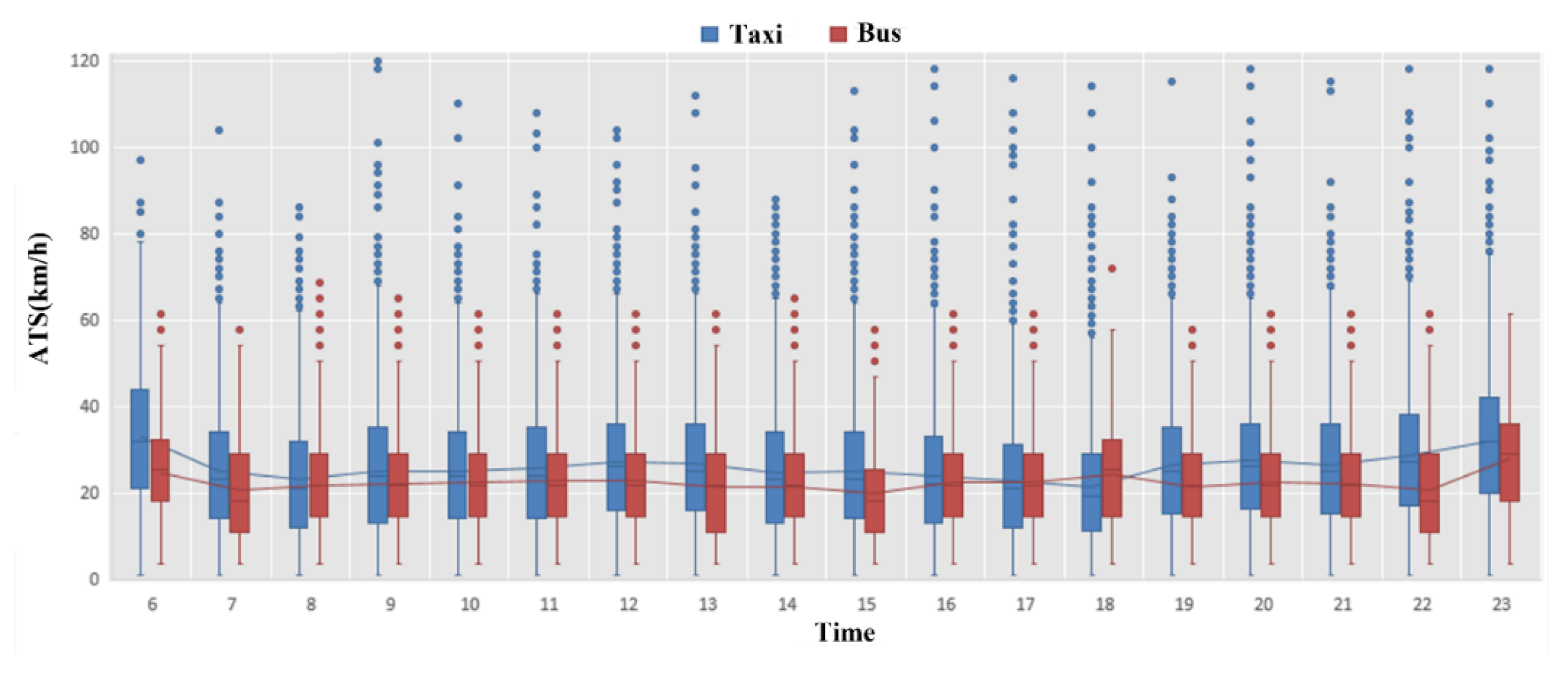
Definition 3. Bus Dwell Time (BDT):Bus dwell time at bus stop i is defined as the time spent for passenger alighting and boarding. The bus dwell time is of great significance to estimate the capacity of a bus station and has also been found to depend on how congested the platform is at the bus stops [35]. The bus dwell time and travel time between adjacent bus stops i and i+1 were estimated by using the method in Reference [36]. Definition 4. Average Travel Speed (ATS):The average travel speed describes the traffic flow status based on the average speed of each bus in an RSB, which can be calculated using the bus trajectory data. The ATS of RSB r in time interval t can be calculated as follows:where spen is the average travel speed of each bus in RSB r in time interval t, and n is the number of buses. Definition 5. Travel Efficiency (TE):Travel efficiency is used to represent passengers’ travel time costs of the RSBs (the time spent of passengers travel from one bus stop to the adjacent stop). The calculation of TE r of RSB r in time interval t is shown as follows: 3.2. Congestion Estimation using an Artificial Neural Network
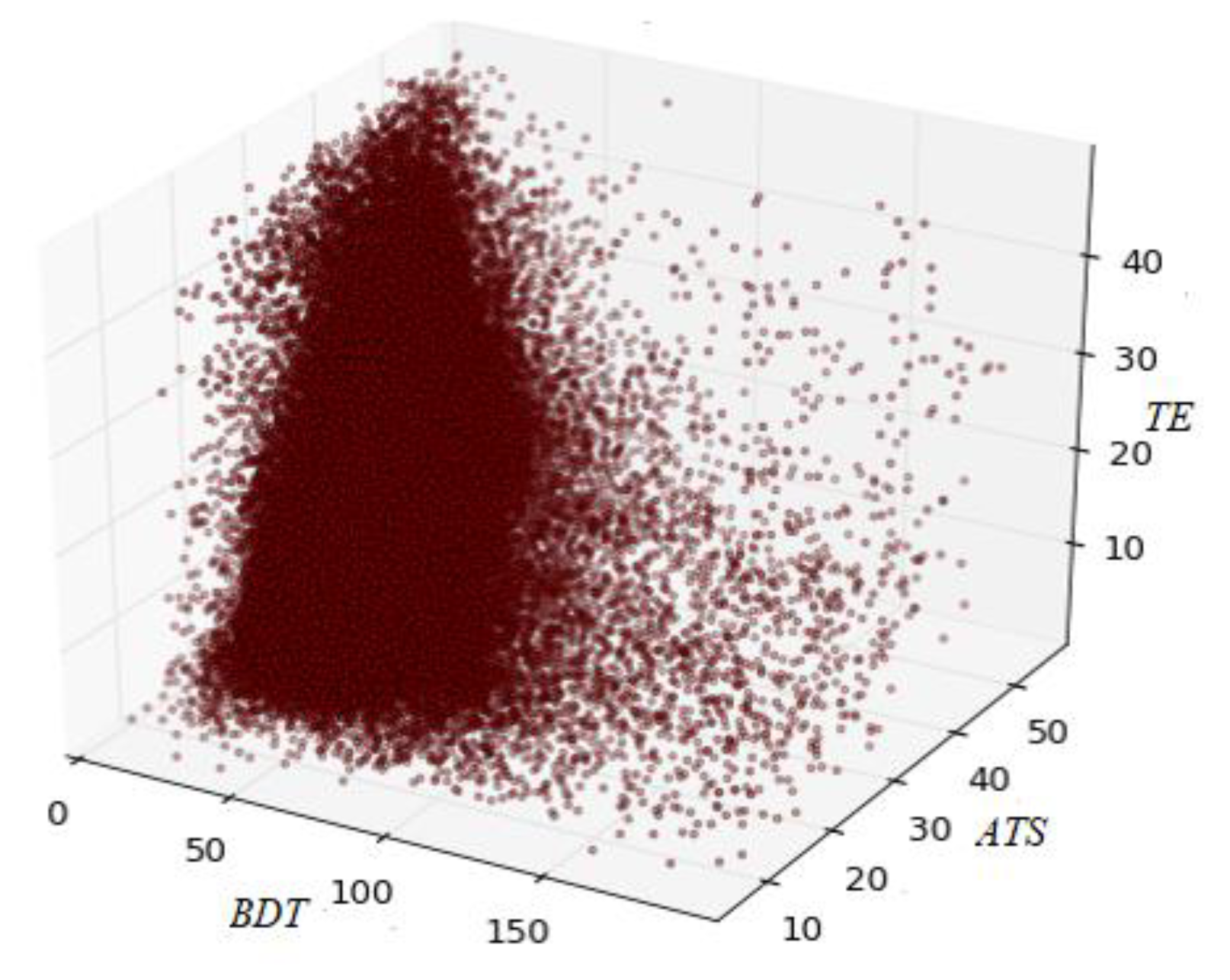
Public traffic congestion usually resulted in slower bus speed and longer travel time. In this study, the three main indicators used to describe the traffic congestion level of the RSBs are BDT, ATS, and TE.
The self-organizing map (SOM) is a type of unsupervised artificial neural network model for the analysis of high-dimensional patterns in data mining applications proposed by Kohonen [
37]. Based on their nearness or similarity, the SOM can classify the objects of the system into clusters, for example categories or regions [
38]. Compared to traditional clustering algorithms, the SOM has three main advantages: 1) prior knowledge is not required; 2) nonlinearity can be handled; and 3) excellent visualization is provided [
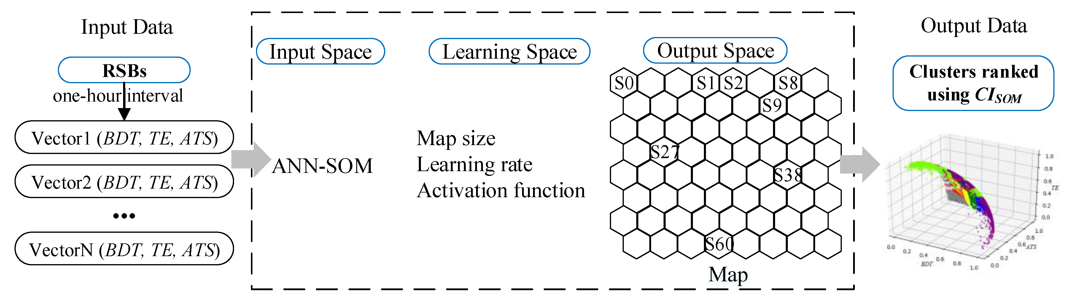
39]. The neurons of the SOM are distributed into two layers: the input layer and the output layer by going through a training phase. In this study, the SOM algorithm is employed to classify the RSBs based on the three traffic indicators, and the Python code is used to complete SOM learning. The flowchart of the SOM used in this study is presented in
Figure 3.
In this study, each RSB comprising three traffic indicators at one-hour interval were sampled simultaneously. All input vectors (three variables:
BDT, ATS, and
TE) were normalized on a scale from 0 to 1. Example vectors of one RSB are shown in
Table 1.
As shown in
Figure 3, the steps of the SOM algorithm are shown as follows [
40]:
- (1)
Initialization: Choose random values for the initial weights
wi, and normalize the input vectors and weights.
where
x = [x1,…,xm]∈
Rm represents an input vector, ||
.|| represents the Euclidean norm, and
M is the number of neurons.
- (2)
Winner Finding: Find the winner neuron
n, using the minimum Euclidean distance between vector
x’ and weights
w i’, according to Equation (5):
- (3)
Update Weights: Adjust the weights of the winner and its neighbors at time
t+1, and renormalize the weights after learning:
where
represents the topological neighborhood function of the winner neuron
n at time
t,
is a positive constant called the ‘‘learning-rate’’,
ri and
rj are the location vectors of nodes
i and
j, respectively.
represents the width of the kernel. The weights are updated at each time step.
- (4)
Algorithm stop condition: Both and will decay over time. The algorithm will stop when or the prespecified number of epochs is reached.
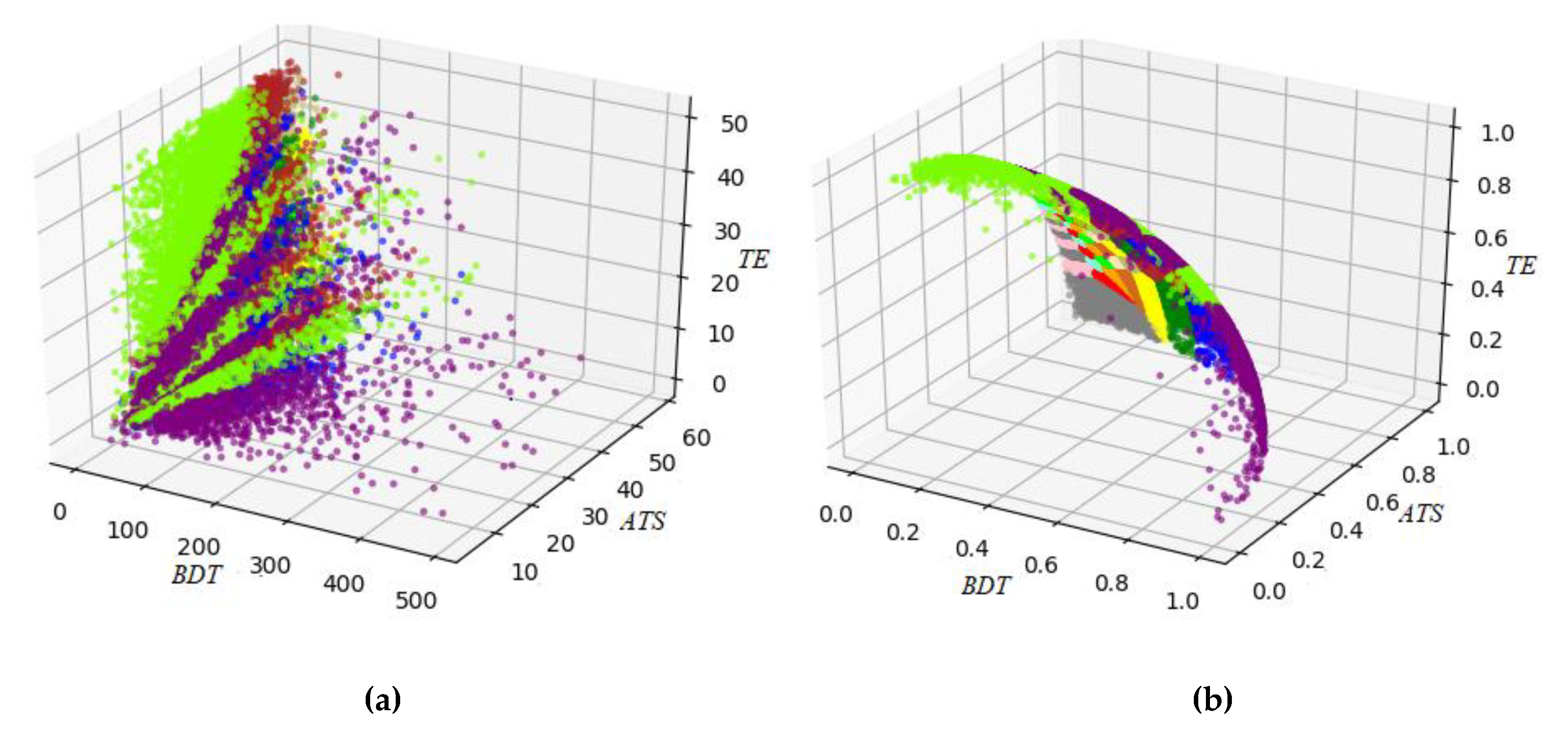
The SOM algorithm provides effective results, which are easily visualized and interpreted from the generated maps [
41]. In general, the traffic condition of the congested RSBs should be positively correlated with the
BDT (the worse the congestion of the RSB is, the longer the travel time is), and negatively correlated with the
TE and
ATS. First, we calculated the mean value of
BDT, ATS, and
TE of all SOM clusters. Then, we developed a congestion index (
CISOM) for ranking each SOM cluster according to Equation (8). In Equation (8), the weight values of
BDT,
TE, and
ATS are set as +1, −1, and −1, respectively.
Next, the resulted clusters of SOM are ranked using CISOM. Consequently, the RSBs in the SOM cluster with the maximum value of CISOM are estimated as the congested RSBs.
6. Conclusions
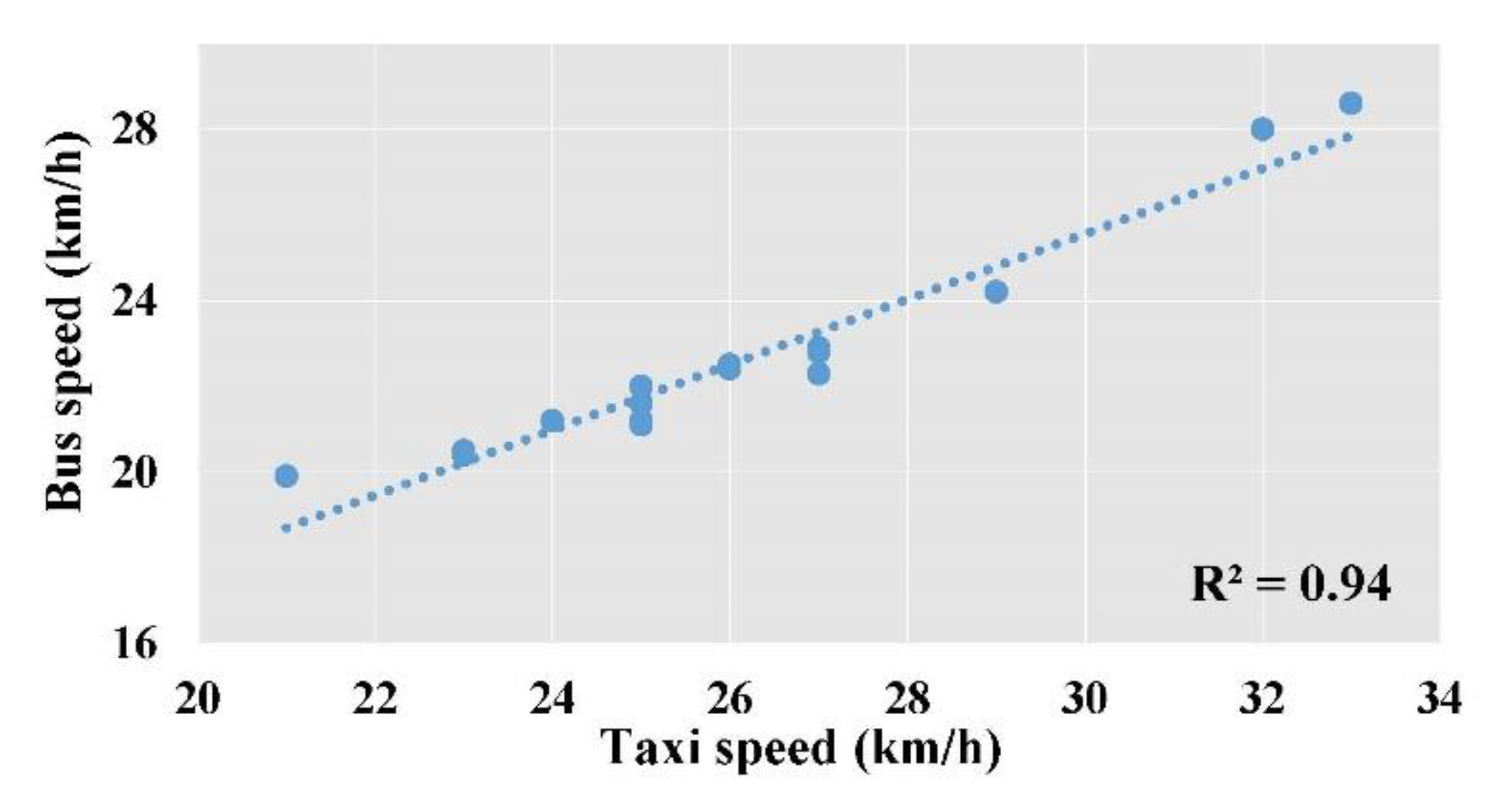
In populated urban regions, the intelligent optimization of PTN plays a prominent role in improving the transport service reliability by alleviating the unpleasant impacts of traffic congestion. In this study, we estimated the traffic congestion of the RSBs based on three traffic indicators: bus dwell time (BDT), average travel speed (ATS), and travel efficiency (TE), which were extracted from SCD and bus trajectory data. In contrast to the previous studies, which focus on the traffic status of one road segment using taxi trajectory data, the aim of our methods was to estimate the traffic congestion of the RSBs using bus trajectory data. Our methodology could be applied to estimate the congested RSBs with bus priority lanes or with limited taxi trips, which can benefit various applications including road traffic status estimation, PTN optimization, and urban transport system management. Based on the congested RSBs, the strategies of public transport network improvement are discussed and evaluated using GA. The results are expected to demonstrate the usefulness of the proposed methodology in sustainable public transport improvements.
Regarding the research limitations, our presented methodology can be applied in a city with a dominating transport mode. However, there are more public transport options (for example, metro system and tram) in major modern cities. Our future research will extend our study to mega-cities, and incorporate the impact of multiple public transport modes and complex network analysis into our methodology [
50]. Moreover, the PTN optimization problem can be subdivided into two major components: the transit routing problem and the transit scheduling problem. Generally, the transit routing problem involves the development of efficient transits routes on an existing road network, with predefined pick-up/drop-off points. On the other hand, the transit scheduling problem is charged with assigning the schedules for the passenger carrying vehicles. In this context, for the PTN optimization process, future work research directions may include other fundamental variables such as bus frequency, vehicle size, function of the public transport headway, and the schedule.


