Abstract
The classification and segmentation of large-scale, sparse, LiDAR point cloud with deep learning are widely used in engineering survey and geoscience. The loose structure and the non-uniform point density are the two major constraints to utilize the sparse point cloud. This paper proposes a lightweight auxiliary network, called the rotated density-based network (RD-Net), and a novel point cloud preprocessing method, Grid Trajectory Box (GT-Box), to solve these problems. The combination of RD-Net and PointNet was used to achieve high-precision 3D classification and segmentation of the sparse point cloud. It emphasizes the importance of the density feature of LiDAR points for 3D object recognition of sparse point cloud. Furthermore, RD-Net plus PointCNN, PointNet, PointCNN, and RD-Net were introduced as comparisons. Public datasets were used to evaluate the performance of the proposed method. The results showed that the RD-Net could significantly improve the performance of sparse point cloud recognition for the coordinate-based network and could improve the classification accuracy to 94% and the segmentation per-accuracy to 70%. Additionally, the results concluded that point-density information has an independent spatial–local correlation and plays an essential role in the process of sparse point cloud recognition.
1. Introduction
1.1. Background
The Light Detection and Ranging (LiDAR) has been widely used for its fast, convenient, and non-contact measurement advantages [1,2,3]. The point cloud is the direct output from a LiDAR sensor, which is a detailed expression of all objects detected by the sensor. Classification and segmentation of large-scale point cloud are substantial topics in geodesy and remote-sensing areas [4,5,6,7,8,9,10,11]. The point cloud has a property called spatially-local correlation, which refers to the dependency relationship within the point cloud [12]. LeCun Yann et al. [13] proposed that mining spatially-local correlation of an object is the key to classification and segmentation through deep learning. Many researchers [14,15,16] have developed various complex network structures to improve the precision of point cloud classification and segmentation, by mining the spatially-local correlation. However, the high-precision requests complex networks, substantial computing parameters, and extended computing time. This complexity changes the LiDAR from a light, real-time measurement technology to heavy and time-consuming data analysis work.
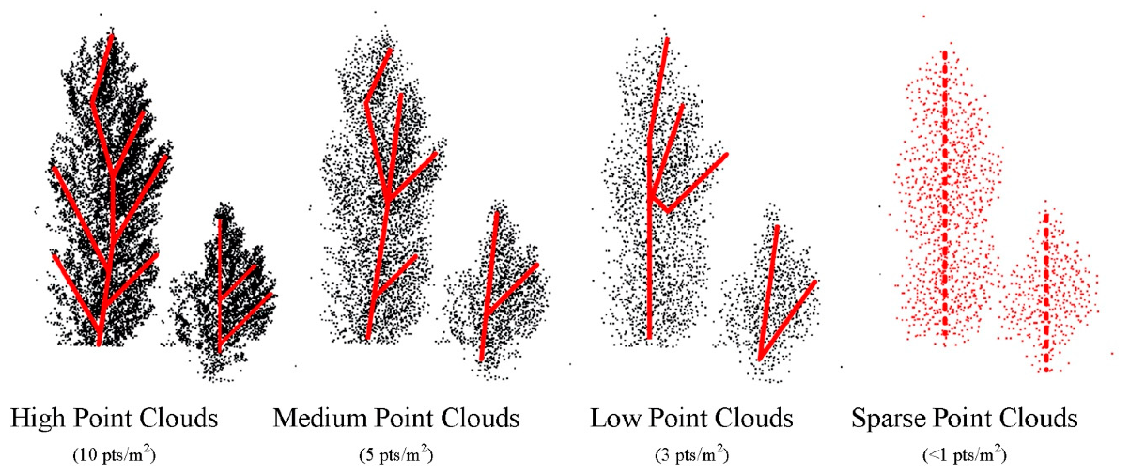
- According to LiDAR specification [17], the point-density defines as the number of points per area where the surface of the earth is sampled. Commonly the point-density is given for one cubic meter (pts/m3). For engineering survey, high, medium, low, and sparse density point cloud is defined as point-density < 2 pts/m3, (2,7] pts/m3, (7,10] pts/m3 and >10 pts/m3, respectively. In order to reduce the computational costs and improve efficiency, many researchers applied the sparse point cloud for classification or segmentation, by using deep learning technology [18,19]. However, applying a sparse point cloud will reduce the amount of data and blur the shape of objects. For large-scale sparse point cloud, with the decrease of the point-density, the shape of the point cloud becomes unclear, the structural feature becomes confused, and the spatially-local correlation becomes difficult to find. Two major constraints to use the sparse point cloud are summarized as: Loose structure: As shown in Figure 1, as the point cloud becomes sparse, the structural features (red dotted line) of the objects become loose. This phenomenon makes it difficult to extract the spatially-local correlation from the sparse point cloud and apply deep learning methods.
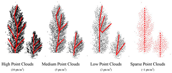 Figure 1. The structural features (red dotted line) of objects in high, medium, low, and sparse point cloud.
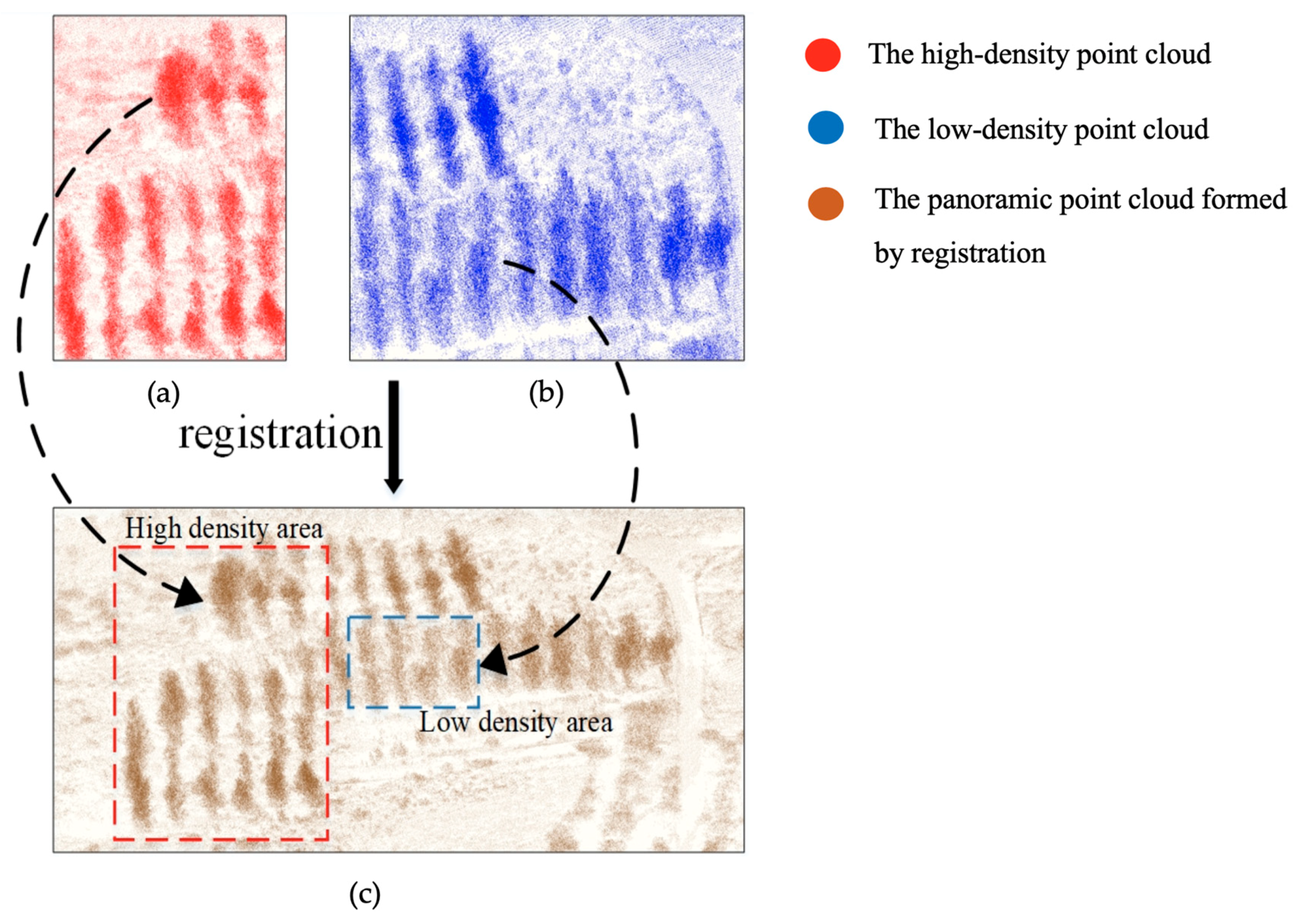
 - Non-uniform point-density: The distribution of point cloud is not uniform since the point cloud is scanned by different scanning stations. The point cloud data of panoramic mining area was obtained by multi-station stitching. This is done by registering the point cloud of different scanning stations in a unified coordinate system. Because the operating mode of Terrestrial Laser Scanning (TLS) is scanning objects through sensor rotation, the point cloud has a scattering characteristic—the point-density is high when the object is close to the sensor and vice versa. The point cloud of the panoramic mining area is spliced together by multiple scanning stations. For a situation where there are many similar objects in a certain area, such as the grove in Figure 2. When a single TLS station is closer to the object, the density is greater, as shown in Figure 2a; when another TLS station is further away from the object, the density is relatively small, as shown in Figure 2b. Therefore, when stitching together, the non-uniform point-density, the difference in point cloud density of the same object in the overlapping area, will be obvious, as shown in Figure 2c.
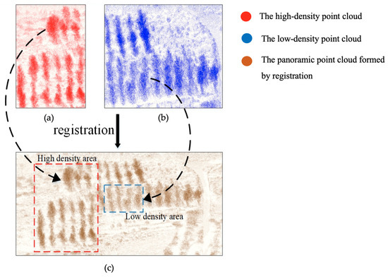 Figure 2. The non-uniform point-density phenomenon. (a) The high-density point cloud obtained when a LiDAR scanning station is close to the grove area. (b) The low-density point cloud obtained when another LiDAR scanning station is far away from the grove area. (c) The Panoramic point cloud formed by the registration of high-density point cloud (red points) and low-density point cloud (blue points).
Besides the two constraints, the points will maintain the relative position to each other, theoretically, when the density of point cloud becomes sparse. This spatially-local correlation reflects the structural feature of the object, which can be used to facilitate the classification and segmentation.
1.2. Related Work
The development of 3D convolutional neural network (3D CNNs) promotes understanding of the semantic analysis of point cloud. Standard convolutional neural networks (CNNs) require dense input representations on uniform grids, but point cloud are sparse and irregular in 3D space. To overcome it, early researchers used volumetric [20,21,22], multi-view [6,23,24,25], or other feature representations in order to first build 3D models. In recent years, the trend has shifted instead to using raw 3D data directly [26,27,28,29,30,31]. Therefore, we divided these approaches into two groups, coordinate-based and feature-based network.
1.2.1. Feature-Based Network
The earlier 3D feature-based network is based on 2D image convolutional models. Many algorithms transform point cloud into features first, then feed in the established CNNs, such as transforming point cloud to regular 3D grids [20,21] or projecting point cloud into a 2D view format [23]. However, these approaches generate a huge volume of unnecessary data and lead to high computational cost during the training process. To enable efficient convolutions, data structures like octrees [32] and voxels [33,34] are utilized. The sophisticated strategies are used to avoid redundant computations. [35,36] encoded in each nonempty voxel with six statistical quantities that are derived from all the points contained within the voxel. VoxelNet [34] designs an end-to-end voxel feature encoding layer to learn a discriminative feature representation from point cloud and predicts accurate 3D bounding boxes. PointPillars [37] encoded features on vertical columns of point cloud to predict 3D oriented boxes for 3D object detection. Recently, more and more networks [15,38,39,40] used multi-feature or multi-modal network models to make up for the deficiency of feature transformation, in a certain way.
1.2.2. Coordinate-Based Network
Coordinate-based networks are end-to-end 3D convolutional models which are directly applied to the point cloud. PointNet [26] is the pioneer in the direct use of raw point cloud for 3D semantic analysis. It involves the skillful use of the max-pooling layer, which is a symmetric function, and the order of points does not affect its output. Max-pooling aggregates point features into a global feature vector, in an order invariance manner. Although the max-pooling idea is proven to be effective, it suffers from the lack of the ability to encode local structures with varying density. Further improvement is followed in PointNet++ [27], in which the weak performance of PointNet in fine-scale segmentation tasks was addressed by the use of multi-scale extraction. PointCNN [12] used coordinate transformation of the point cloud to simultaneously weight and permute the input features. SO-Net [29] explicitly utilizes the spatial distribution of input point cloud during hierarchical feature extraction. EdgeConv [30] used a dynamic graph CNN operator to better capture the local geometric features of point cloud, while maintaining permutation invariance. However, these network all focus on the analysis of dense point cloud, scanned at small-scale scenario like indoor spaces (ModelNet40, ScanNet [41]). The applications of the point cloud in the large-scale scene has not been well-investigated.
1.3. Contributions
This paper proposed a data preprocessing method—a Grid Trajectory Box (GT-Box)—and a lightweight density feature-based (density-based) network—Rotated Density Network (RD-Net), to analyze the large-scale sparse point cloud. The remainder of the paper is organized as follows: The formulation of GT-Box preprocessing and RD-Net is introduced in Section 2. In Section 3, the proposed method is tested and compared with other existing methods. The results and discussion are presented in Section 4. Finally, conclusions are offered in Section 5.
2. Methodology
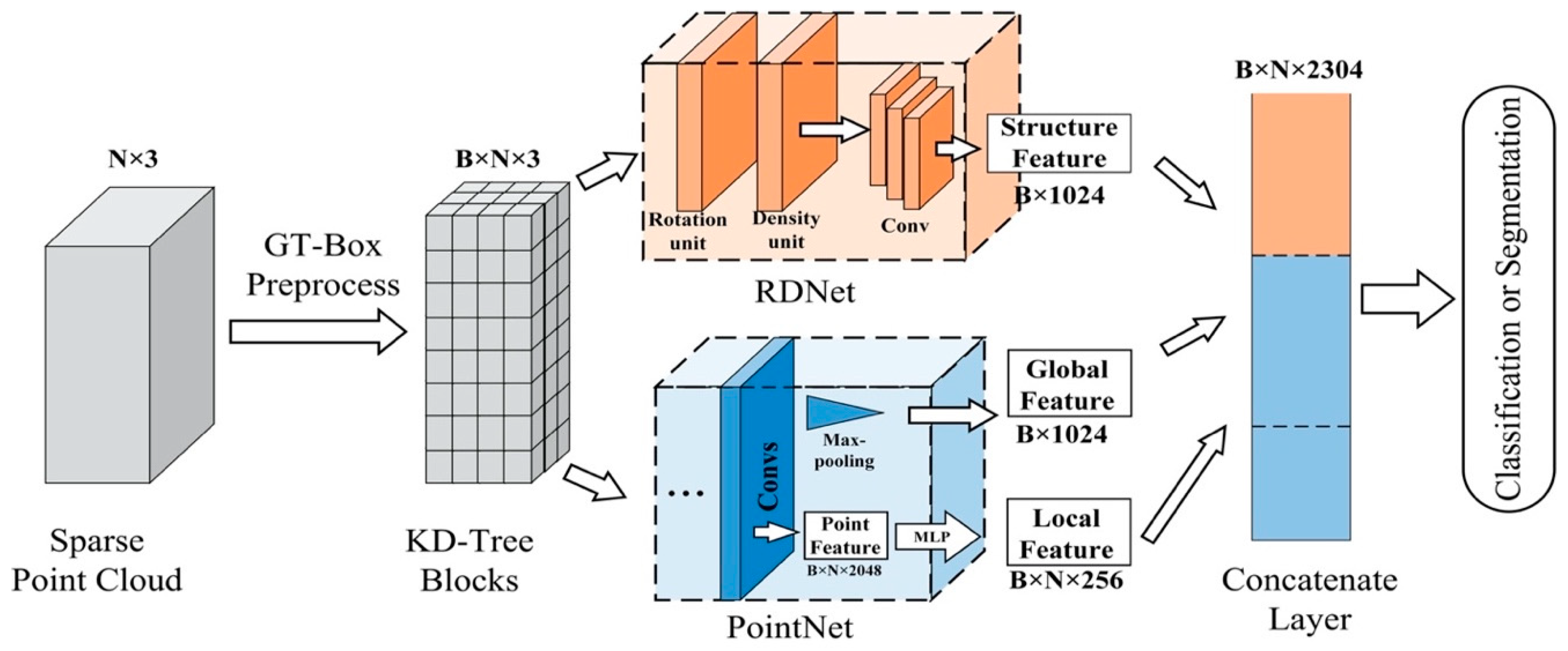
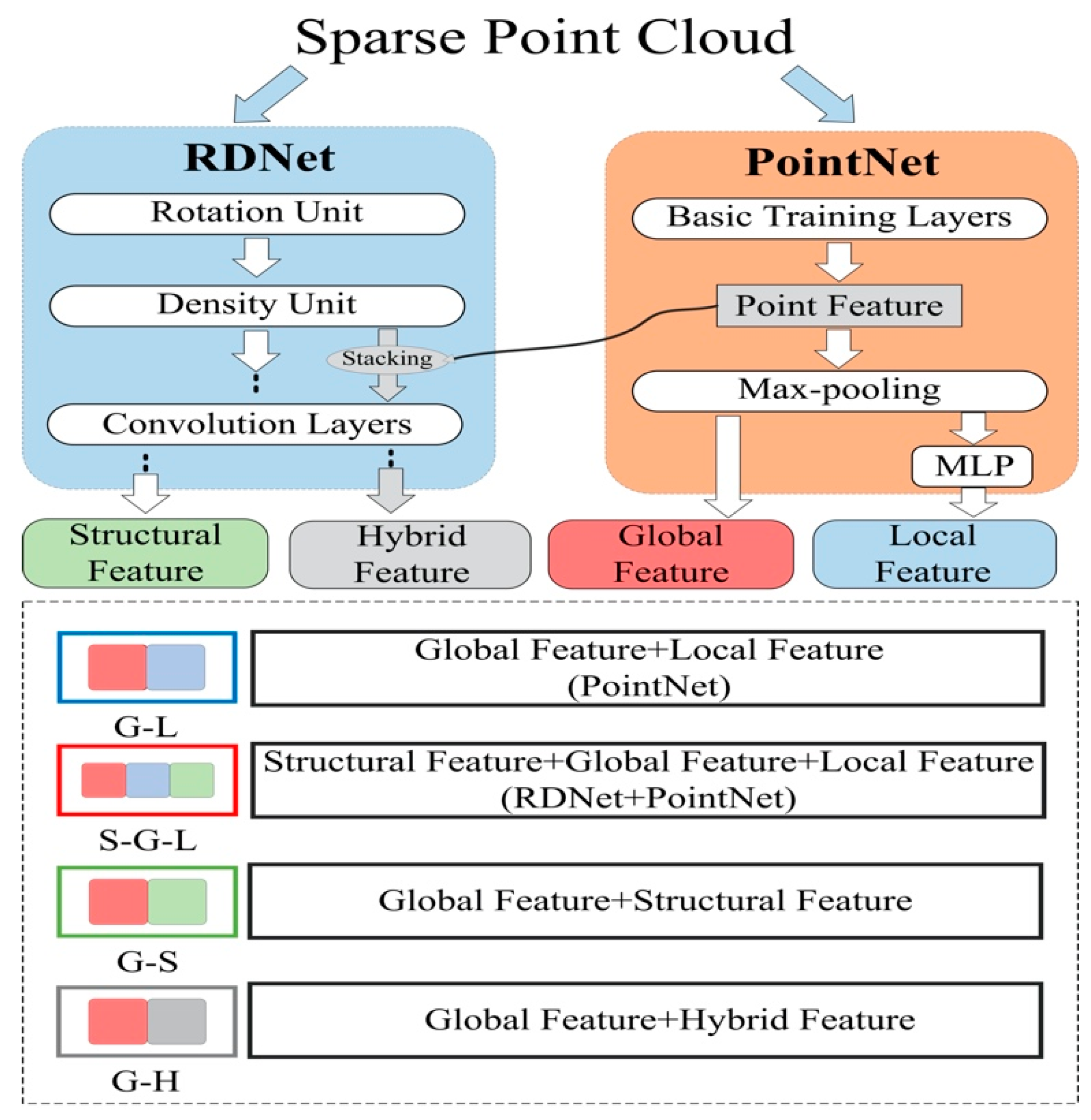
First, we introduce GT-Box preprocess to divide the input sparse point cloud into K-Dimensional-Tree blocks (KD-Tree blocks) as training data in Section 2.1. Then, the description of our network, Rotated Density Network (RD-Net) is presented in Section 2.2. Finally, in Section 2.3, the most efficient semantic analysis method, RD-Net+PointNet, is done to achieve high-precision classification and segmentation of large-scale sparse point cloud. The overall information flow of RD-Net+PointNet is shown in Figure 3. RD-Net+PointNet is a multi-feature (structural feature, global feature, local feature) network combining GT-Box preprocess, density-based network RD-Net and coordinate-based network PointNet. The complete information flow is described in detail.

Figure 3.
The overall information flow of rotated density-based network (RD-Net)+PointNet.
2.1. GT-Box Preprocess
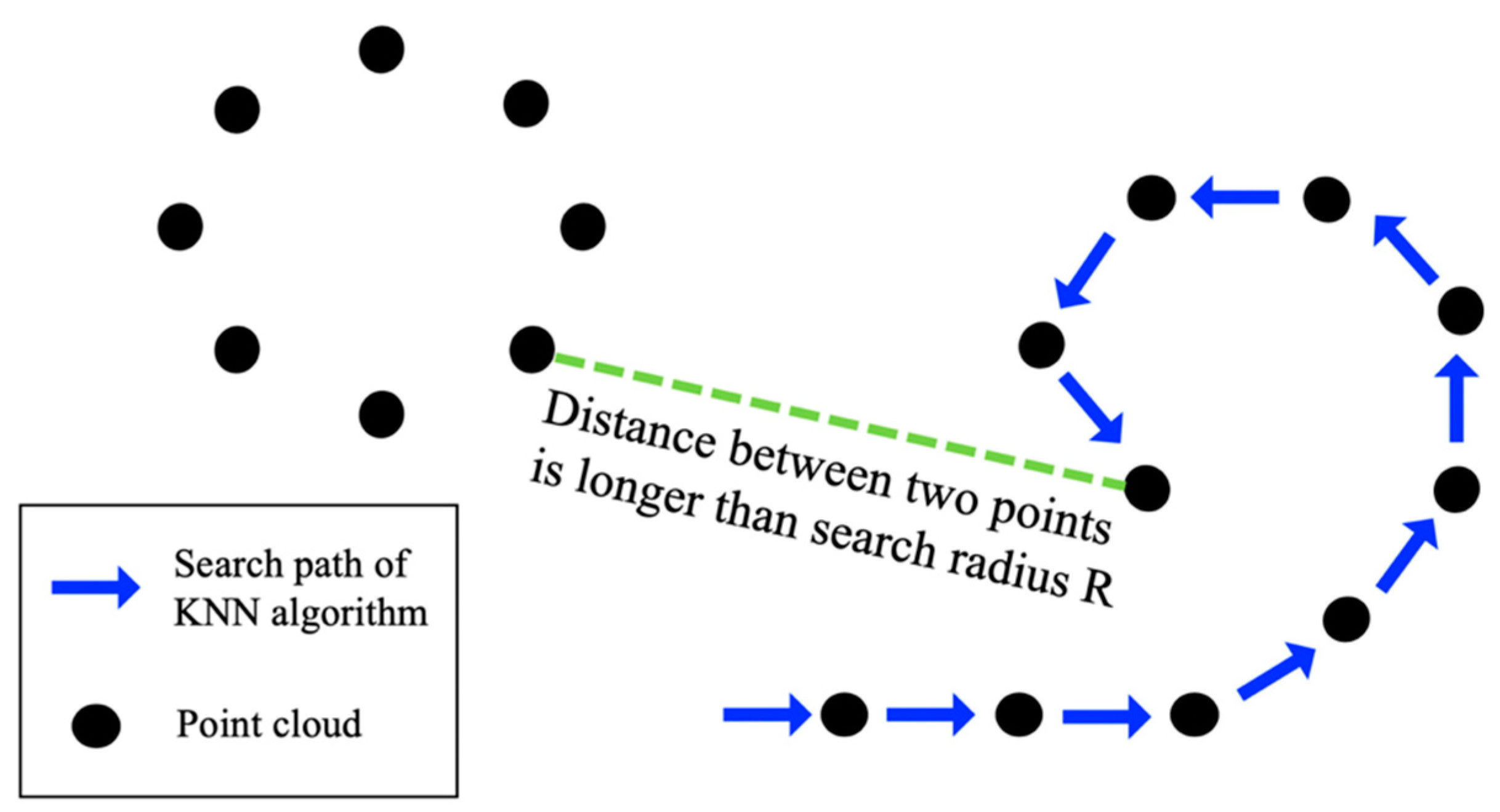
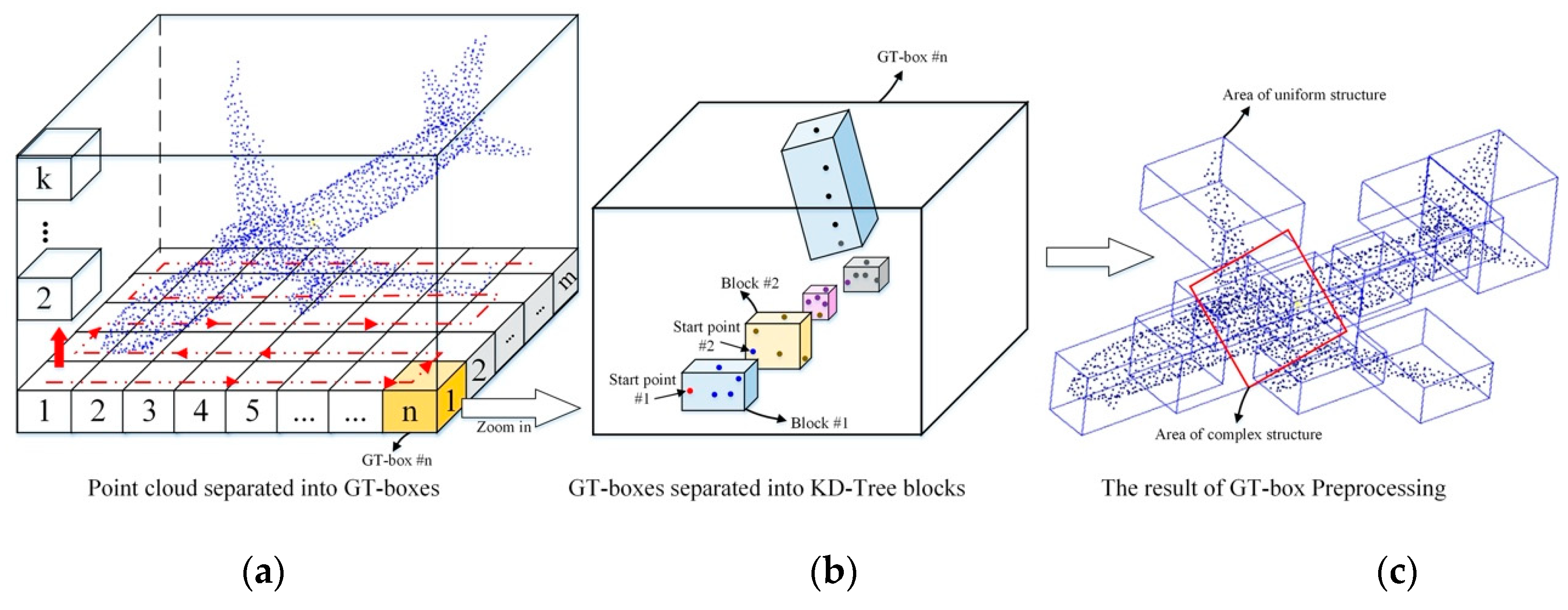
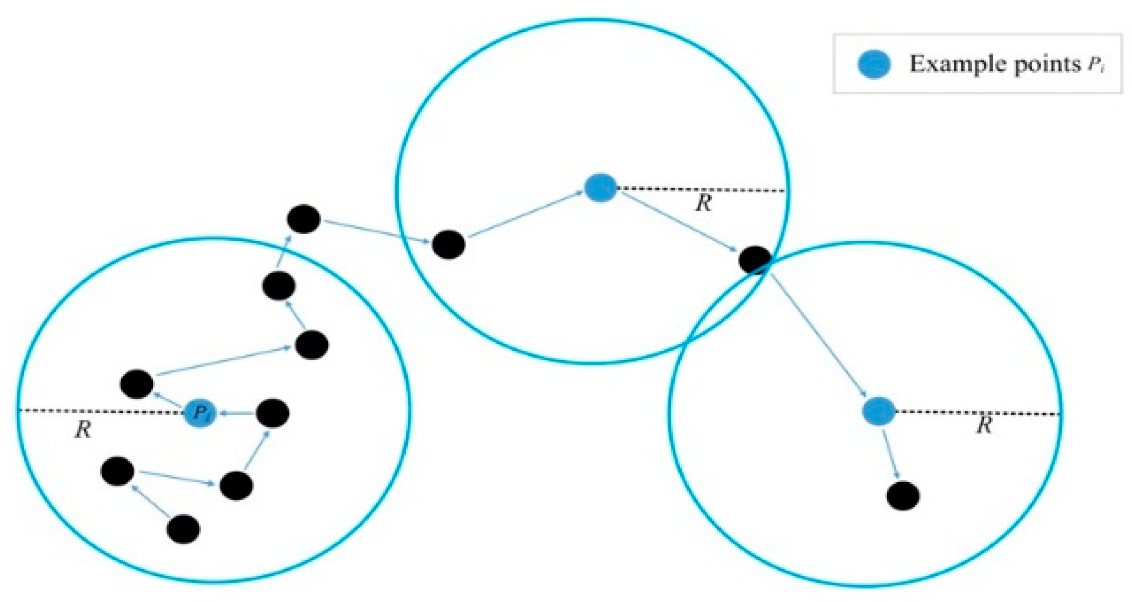
GT-Box preprocess is developed to maintain the spatial structure of point cloud, as well as transform large-scale point cloud into a standard input size, without any overlap area. Through GT-Box preprocess, the point cloud is separated into many regular KD-Tree blocks, which facilitates the high-dimensional information computed in a convolution subsampling operator. Specifically, the GT-Box preprocess includes two steps—building GT-Boxes and generating KD-Tree blocks, based on K-Nearest Neighbor (KNN). The purpose of building GT-Boxes is to fix the search range of the KNN algorithm, and prevent the algorithm from getting stuck in a local area, when using the KNN algorithm to find the nearest neighbors in the second step. In Step 2 (Generating KD-Tree blocks), we first set the appropriate search radius R, and stipulate that each round of search must traverse all points in the current GT-Box, make sure that there are no points with a distance smaller than the search radius R from the previous point, before entering the next GT-Box. As the point spacing in large-scale sparse point cloud is quite different, if we do not use Step 1 (Building GT-Boxes), it might cause a bug that the KNN algorithm can only search in a certain local area, and cannot complete the jump operation when the point spacing is greater than the search radius R, as shown in Figure 4.
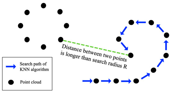
Figure 4.
An example of the application bug of the K-Nearest Neighbor (KNN) Algorithm in sparse point cloud.
2.1.1. Building GT-Boxes
GT-Box is a traversal box that divides the point cloud into boxes with the same size. When we choose the dimensions of the GT-Boxes, we should avoid the fault–point clouds gathered at different edges, with obvious gaps in the middle—in the GT-Box, as much as possible, and the S-type traversal rule is used to identify the boxes, as shown in Figure 5a. For example, the large-scale point cloud size of the mining subsidence basin scene is 1342.46 × 1245.2 × 85.75 m3; in Section 3. Among the objects that we want to classify or segment are many strip structures, such as buildings and trees. Therefore, we also divided the unit GT-Boxes into a strip structure. The length and width of the unit GT-Box were defined as one-hundredth of the boundary of the sparse point cloud, the height of the unit GT-Box was designated as one-fifth of the height of the sparse point cloud, 13.42 × 12.45 × 17.15 m3. With this operation, the point cloud is divided into a number of fixed search regions, named GT-Boxes. The identification of the GT-Boxes is to be used in the sampling process, for the next step.
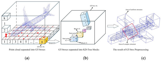
Figure 5.
Grid Trajectory-Box (GT-Box) preprocess of KNN. (a) GT-Box traversal—Point cloud separated into GT-Boxes; (b) KNN sampling—GT-Boxes separated into K-Dimensional-Tree blocks (KD-Tree blocks); and (c) the results of GT-Box preprocessing.
2.1.2. Generating KD-Tree Blocks
KNN clustering algorithm is used to divide each GT-Box into many KD-Tree blocks. First, we take the first point in the box as the starting point and search the nearest K points. The first K-1 points and the starting point are combined as the KD-Tree block. Then, the Kth point will be used as the starting point for the next combination. When the number of points in the box is less than the threshold K (K depends on the points input to the KNN), the processing of this GT-Box is finished.
After this operation, all objects in the sparse point cloud is divided into many KD-Tree blocks, which have the same number of points but different space sizes, as displayed in Figure 5b,c. If the structure of an object is simple and the point-density is uniform, the size of the KD-Tree block is large and the point distribution is uniform. On the other hand, if the structure is complex and the point-density is uneven, the size of the KD-Tree block is small. By GT-Box preprocess, we separate sparse point cloud into training samples in a standard format, while maintaining the structural features of objects.
2.2. RD-Net
RD-Net is a lightweight density-based network. It is combined with two key units—the point-density unit and the rotation unit. This network enhances the spatially-local correlation by extracting the structure features from point-density information. The point-density information reflects the relationship among each point.
Specifically, RD-Net operation includes the rotation unit, the density unit, and the lightweight training layers, as shown in Figure 6.
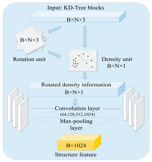
Figure 6.
The structure frame of RD-Net. The input KD blocks are the matrix with BxNx3 shape. B means the number of batch size, N means the number of points, and 3 means the three dimensions (x, y, z).
2.2.1. Rotation Unit
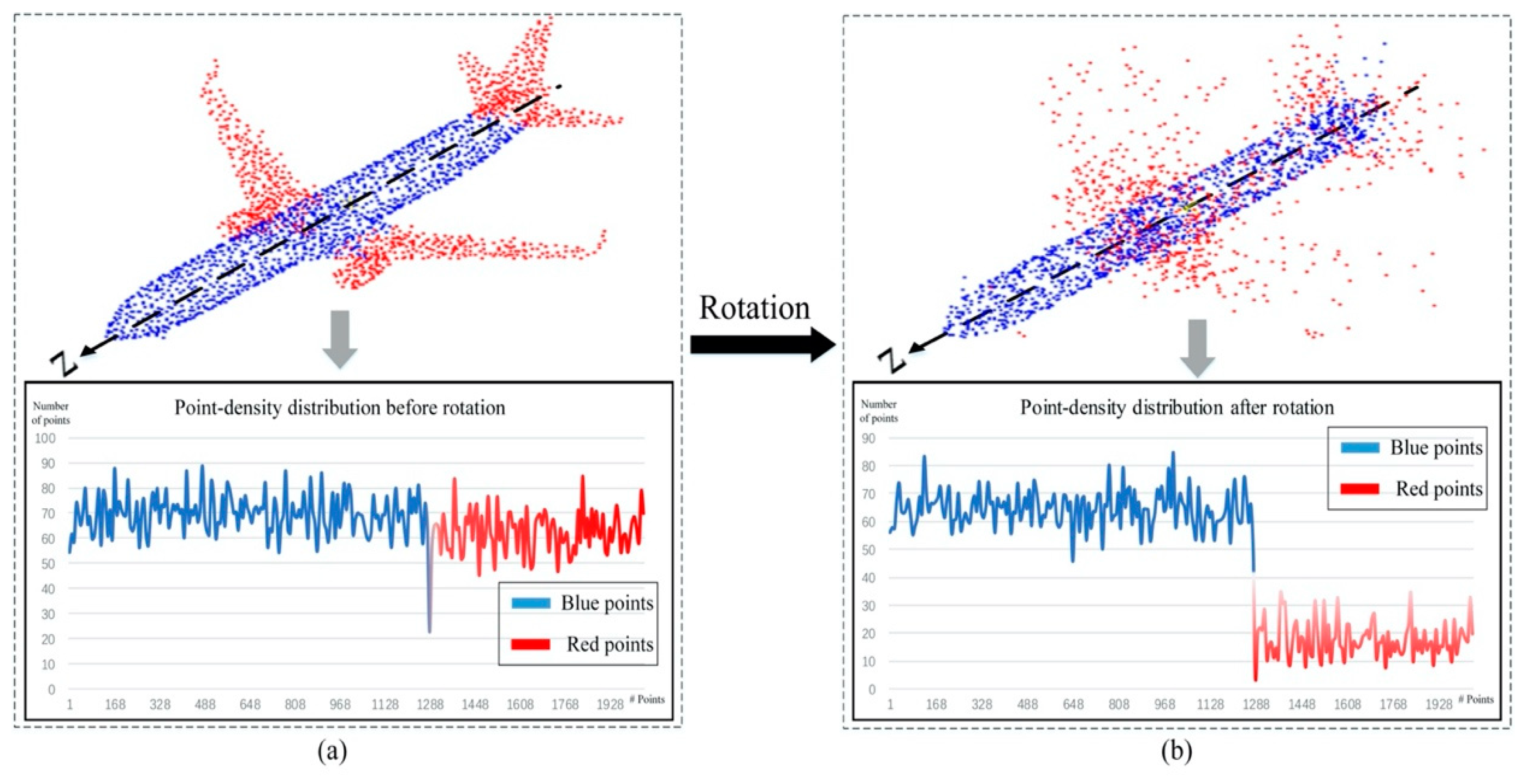
An object usually consists of several KD-Tree blocks, as shown in Figure 5c. The rotation unit changes the density information of the object by rotating the KD-tree blocks with random angles, along the rotation axis (Z-axis in Figure 7). Specifically, in Figure 7, we use color to divide the point cloud into structure points (the points distribution is consistent with the rotation axis, blue points) and the non-structure points (the points distribution is inconsistent with the rotation axis, red points). When the data passes through the rotation unit, because the distribution of structure points is consistent with the rotation axis, the point density changes little; as shown in in Figure 7, blue curve. On the contrary, rotation of unstructured points causes dramatic point-density distribution changes, as shown in Figure 7, red curve. According to this phenomenon, the delta of the point-density distribution, before and after the rotation can be used to identify the structure feature.
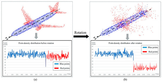
Figure 7.
The rotation unit of RD-Net. (a) Point-density information of object before the rotation. (b) Point-density information of object after the rotation.
2.2.2. Density Unit
According to [13], the external shape feature and the internal structure feature of the object are independent. In order to separate the two structures, we defined point-density information by calculating the point-density of each point and organize the result to a one-dimensional matrix.
To calculate the density of each point, the radius parameter R of the region needs to be selected properly, as shown in Figure 8. Through the k-query algorithm [42], we traversed each point in the input KD-Tree block sample and calculated the number of points n in the spherical volume V with radius R, and their relative distance {d} from the center point. Dividing n(pts) by V(m3), the point-density information is obtained as the input data; dividing {d}(m) by n(pts), the distance information is obtained as the bias of the CNN layers in the RD-Net. The volume calculation formula of the unit sphere is as shown in Equations (1) and (2).
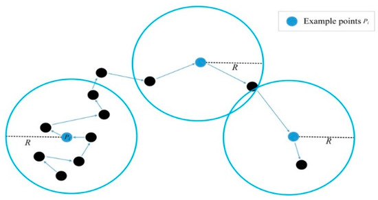
Figure 8.
The calculation process of point-density in density unit. R is the radius of the unit sphere.
Through density unit, we divided the points from KD-Tree blocks into two types, according to the point-density. Structural points and non-structural points. The structure points are at the intersection of object structures with high and uneven point-density. The non-structural points are with the single structural feature, uniform point-density. Therefore, similar objects have similar structural features.
where, is the ith point in the KD-Tree block, represents the number of adjacent points through the k-query algorithm. is the radius of the unit sphere.
2.2.3. The Implementation of RD-Net
First, the point cloud is rotated in the rotation unit, as shown in Equations (3) and (4).
where, is the rotation matrix with the rotation angle along with the Z-axis, represents the input point cloud, and represents the rotated point cloud.
Then, the two sets of point cloud, before and after the rotation, are transferred to the density unit to calculate the point-density, as shown in Equation (5).
where represents the matrix of the density of point cloud.
Finally, the point-density information is transferred into lightweight convolution layer for training, as shown in Equations (6) and (7).
where represents high-dimensional information through the network, represents the multi-layer perceptron, is the symmetric function of max-pooling.
2.3. Semantic Analysis with RD-Net+Coordinate-Based Network
We combine the result from RD-Net with the PointNet to perform the semantic analysis. PointNet is an end-to-end network that directly analyses point cloud, based on coordinates, which transforms coordinate information into three different features (Global Feature, Point Feature, and Local Feature), as shown in Figure 3.
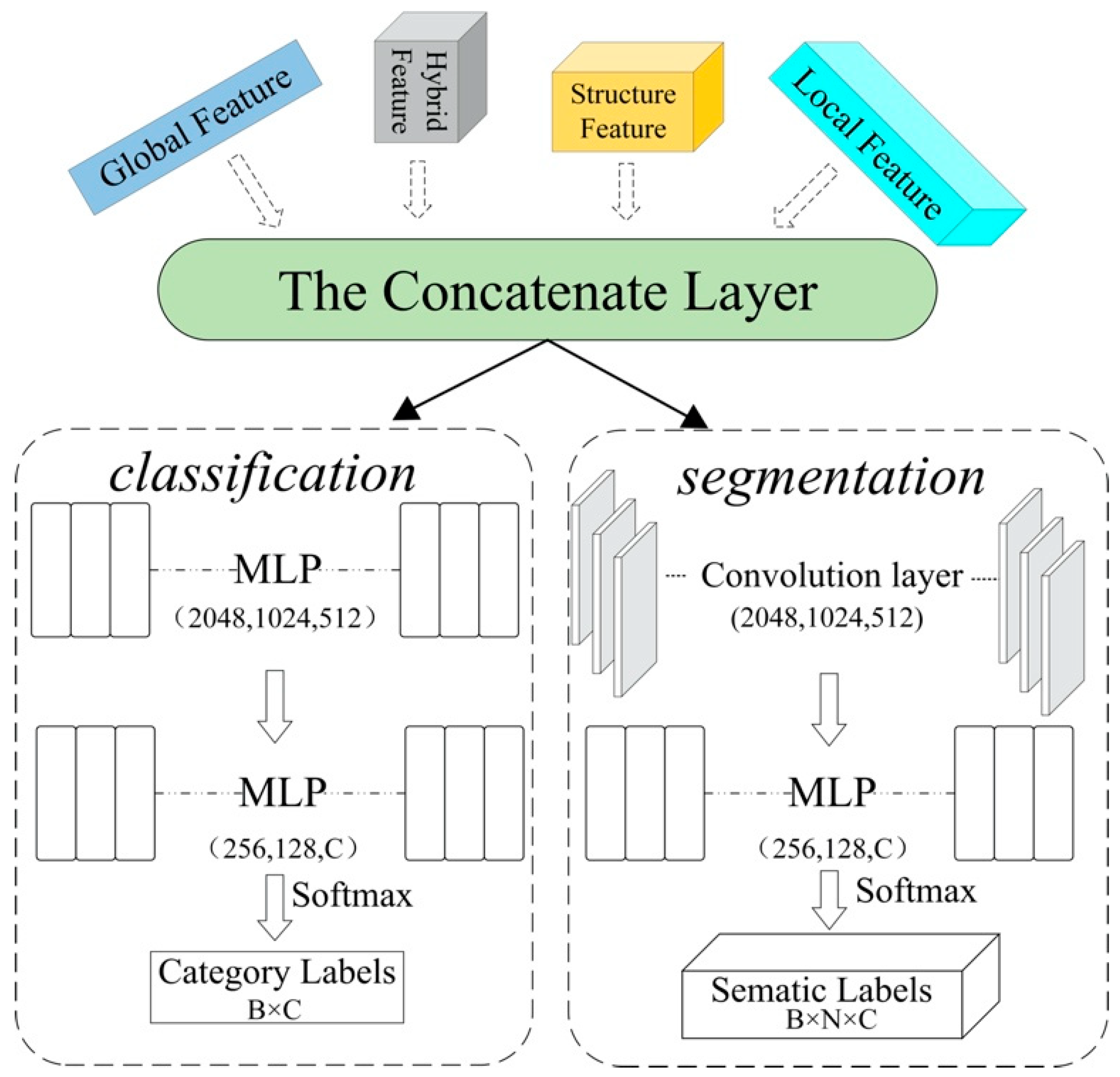
Through the RD-Net and PointNet, we can obtain four distinct features—the global feature (B, 1024), the point feature, the local feature (B, N, 256), and the structural feature (B, 1024). The global feature has a large-scale and represents the entire spatial shape of KD-Tree blocks, and the local feature has a small-scale and represents a local region shape of KD-Tree blocks. The structural feature is from the RD-Net, which has a large-scale and analyses the topological relationship of the entire sample block. We selected structure feature and global feature N times, to form a matrix of the same shape as (B, N, 1024). Then, we stacked them together as input data (B, N, 2304) for classification or segmentation in the concatenate layer, as shown in Figure 3. Then, we applied different training layers to these two kinds of tasks, as shown in Figure 9.
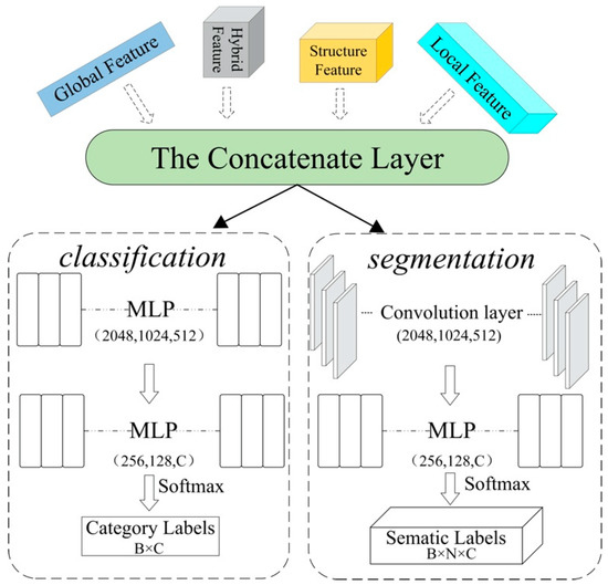
Figure 9.
The structure of Classification (left) and Segmentation (right). The classification task outputs the overall category of each block. The segmentation task outputs categories for each point.
For classification, a network with sufficiently strong feature analysis capabilities performs steadily in classification tasks. In classification, the entire input is classified into different categories. Through the multi-layer perceptron (MLP), high-dimensional information (2048) is converted into certain-dimension predictive category C of the input point cloud. In addition, the output is a classification result with C × 1 one-hot vector, C representing the classification categories.
For segmentation, this task requests the sensitivity to the change of features. In segmentation, every point in KD-Tree blocks needs to be predicted. As such, we labeled every point in the input separately. Through CNN layers and MLP, the output is a B×N×C matrix, where N is the number of points.
3. Materials and Experiments
3.1. Datasets
The point cloud of two scenes, rural scene and large-scale mining subsidence basin scene is used to evaluate the proposed method, as the experimental data. The data of each scene is divided into different point-density scales by down-sampling.
(1) Rural scene: We selected rural scene data from Semantic3D [43]. Through down-sampling, the data are processed into four point-density levels—high, medium, low, and sparse density point cloud, as shown in Table 1. The object label has 8 different categories—natural terrain, high vegetation, low vegetation, buildings, hard scape, scanning artifacts, and cars.

Table 1.
Input data sets of experiments.
(2) Large-scale mining subsidence basin scene: The measured point cloud of Shandong mining area in Ordos China is used as the data sets. The original point cloud was obtained by multi-station registration using TLS Rigel VZ-4000 LiDAR sensors with high-resolution 300 MHZ scanning. Three times surveys for the same mining area, from summer to autumn, four months in total (May 28, 2018; July 3, 2018; and September 10, 2018) are used. The data were sub-sampled into four point-density levels, high, medium, low, and sparse density point cloud, as displayed in Table 1. The point cloud of mining area mainly contain terrain, vegetation, and building categories. The sizes of the files are also shown in Table 1.
3.2. Implementation Details
We used the same framework and training strategy to perform independent experiments on four density types of point clouds (high, medium, low, and sparse). Each density type of data has two different scene of point cloud, rural and mining subsidence basin. In the GT-Boxes preprocessing phase, we divided the point cloud into GT-Boxes, then generated KD-Tree blocks, as experiment samples, based on those GT-Boxes. In particular, we applied a unit GT-Box with dimensions of 2.46 × 2.25 × 12.89 m3 for the rural scene and 13.42 × 12.45 × 17.15 m3 for the mining subsidence basin scene, respectively. We, respectively, divided the rural scene and the mining subsidence basin scene point clouds into 2500 GT-Boxes and 9400 GT-Boxes, for each density type. The KD-Tree blocks generated by these GT-Boxes were used as samples for our experiment, as shown in Figure 10. In order to observe the influence of different density type of point cloud on our proposed network more objectively, we selected 33,200 KD-Tree blocks, 10,000 from rural scenes, and 23,200 from mining subsidence basin scenes, for each density type of point cloud, as experimental samples. For classification tasks, each sample is described as a one-dimensional one-hot vector ([1,3] for mining subsidence basin scene, [1,8] for rural scene). For segmentation tasks, each sample is described as an n-dimensional one-hot vector (n represents the number of points, [n, 3] for mining subsidence basin scene, [n, 8] for rural scene). Then, we divided the data into 25,000 training data sets and 8200 test data sets by random sampling, according to the ratio of 3:1. Before the training phase, we used the rotated unit to compare the change of the density of point cloud before and after rotation, from a small part of the point cloud samples of each category, to find the most suitable radius parameter R. The loss function uses multi-category cross entropy.
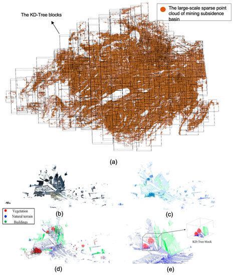
Figure 10.
Point cloud recognition details in two different scenes. (a) Mining subsidence basin sparse point cloud is divided into KD-Tree blocks by GT-Boxes preprocessing. (b) An original point cloud of the rural scene of Semantic3D. (c) Sparse point cloud is generated by sub-sampling the original point cloud. (d) Through GT-Box preprocessing, the boxes are more in the places with dense points (vegetation, buildings) and less in the places with uniform points (terrain). (e) The result of segmentation by RD-Net+PointNet.
The experimental tests were conducted by a computer equipped with a 64-bit Intel Core i5- 6300HQ CPU at 2.3 GHz, GeForce GTX 950M GPU, and 12 GB RAM, running the Ubuntu 18.04 operating system. All proposed methods were implemented using Tensorflow-GPU 2.0.0. In our proposed method, the activation function of the hidden layer uses ReLU, the activation function of the output layer uses SoftMax, and the training process uses the Adam optimizer, with an initial learning rate 0.005. The learning parameters were optimized using dropout, batch normalization, and an exponentially decaying learning rate.
3.3. Design of Experiments
To evaluate the performance of RD-Net and the impact of point-density information on the deep learning process, three series of experimental tests were conducted.
For classification, the running time and classification accuracy were recorded for each epoch. The classification accuracy is equal to the number of correct predictions divided by the total number of samples. The average accuracy of samples is used to evaluate the classification task. For segmentation, the accuracy is equal to the number of correct predicted points in this block divided by the total number of points in this block. The average segmentation accuracy and the mean Intersection over Union (mean-IoU) are used to evaluate the segmentation task performance.
3.3.1. Experiment 1: Performance Evaluation on RD-Net
The proposed method, RD-Net, is an auxiliary density-based network. It can be efficiently used in the mining scene by quickly identifying the density characteristics of point cloud and combining them with the original pre-training coordinated-based network, such as PointNet and PointCNN, it can achieve efficient recognition level for large-scale sparse point cloud. Based on this view, we combine RD-Net with current popular end-to-end coordinate-based networks, PointNet and PointNet, to form RD-Net+PointNet and RD-Net+PointCNN. We designed two experiments (E 1.1, E 1.2) to analyze the performance of RD-Net and the properties of point-density information from different perspectives.
(E1.1) We applied five different network, PointNet, PointCNN, RD-Net, RD-Net+PointNet, and RD-Net+PointCNN, to carry on the comparative experiment of classification and segmentation. Classification accuracy and Mean-IoU were used to evaluate the performance. All five methods were applied to the sparse point cloud of both scenes. Then, the best performing network in this experiment, RD-Net+PointNet, was applied to the mining subsidence basin data set, to compare the performance on classification.
(E1.2) Different combination modes of the four internal features of RD-Net+PointNet are tested in this experiment. The goal is to identify the importance of each feature. The combination modes are shown in Figure 11. In which, G-L: Global Feature + Local Feature combination mode; the S-G-L: Structural Feature + Global Feature + Local Feature; the G-S: Global Feature + Structural Feature combination mode; and the G-H Global Feature + Hybrid Feature combination mode.
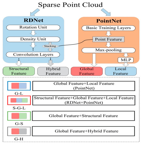
Figure 11.
Information flow of different feature combinations.
3.3.2. Experiment 2: Evaluate the Effect of Radius Parameter R
Different values of radius parameter R of the unit sphere in density unit were tested in this experiment.
3.3.3. Experiment 3: Performance Evaluation on Different Density Type of Point Cloud
To verify the impact of different data volumes on efficiency. We applied the same training strategy to classify four different density types of point cloud (high, medium, low, and sparse) using the best performing network in this experiment, RD-Net+PointNet. Furthermore, we also tested the point cloud of different densities with four different combination modes.
4. Results and Discussion
In this section, the experiments results are presented and discussed, respectively.
4.1. Results and Discussion on Experiment 1
(E 1.1) The classification and segmentation results of RD-Net+PointNet for mining subsidence basin data set are shown in the Figure 12. The evaluation results for different methods are shown in Table 2. Density-based network, RD-Net, could significantly improve the performance of large-scale sparse point cloud recognition for the coordinate-based network, such as PointNet and PointCNN. For the mining subsidence basin scene, RD-Net+PointNet showed the best performance in both classification and segmentation tasks. The classification accuracy and the mean-IoU were 94.06% and 83.41%, respectively; followed by the PointNet method with 90.10% classification accuracy and 80.73% mean-IoU. The same performance could be observed in the rural scene. RD-Net recognizes objects from the perspective of spatial structure by analyzing the density characteristics. It does not depend on the coordinates of the point cloud itself, but is analyzed by the relative position relationship between the points, which is independent of the coordinate-based network. Therefore, compared with the traditional end-to-end coordinate-based network, such as PointNet and PointCNN, the network combining RD-Net is more robust. In addition, RD-Net is a lightweight network with a small number of weight parameters and low calculation costs. Combining traditional networks with RD-Net, such as RD-Net+PointNet, could help researchers to apply it more efficiently to different scenarios. The superior performance demonstrated the high-precision semantic analysis of large-scale sparse point cloud, by combining the RD-Net and PointNet. Table 2 also illustrates that the RD-Net should be used with another coordinated-based network (PointNet or PointCNN).

Figure 12.
Recognition results of sparse point cloud (Mining subsidence basin). Classified and segmented large-scale sparse point cloud, through our proposed method, RD-Net+PointNet.

Table 2.
Comparison of different methods for sparse point cloud (Mining and rural scene). Calculate both classification and mean-IoU.
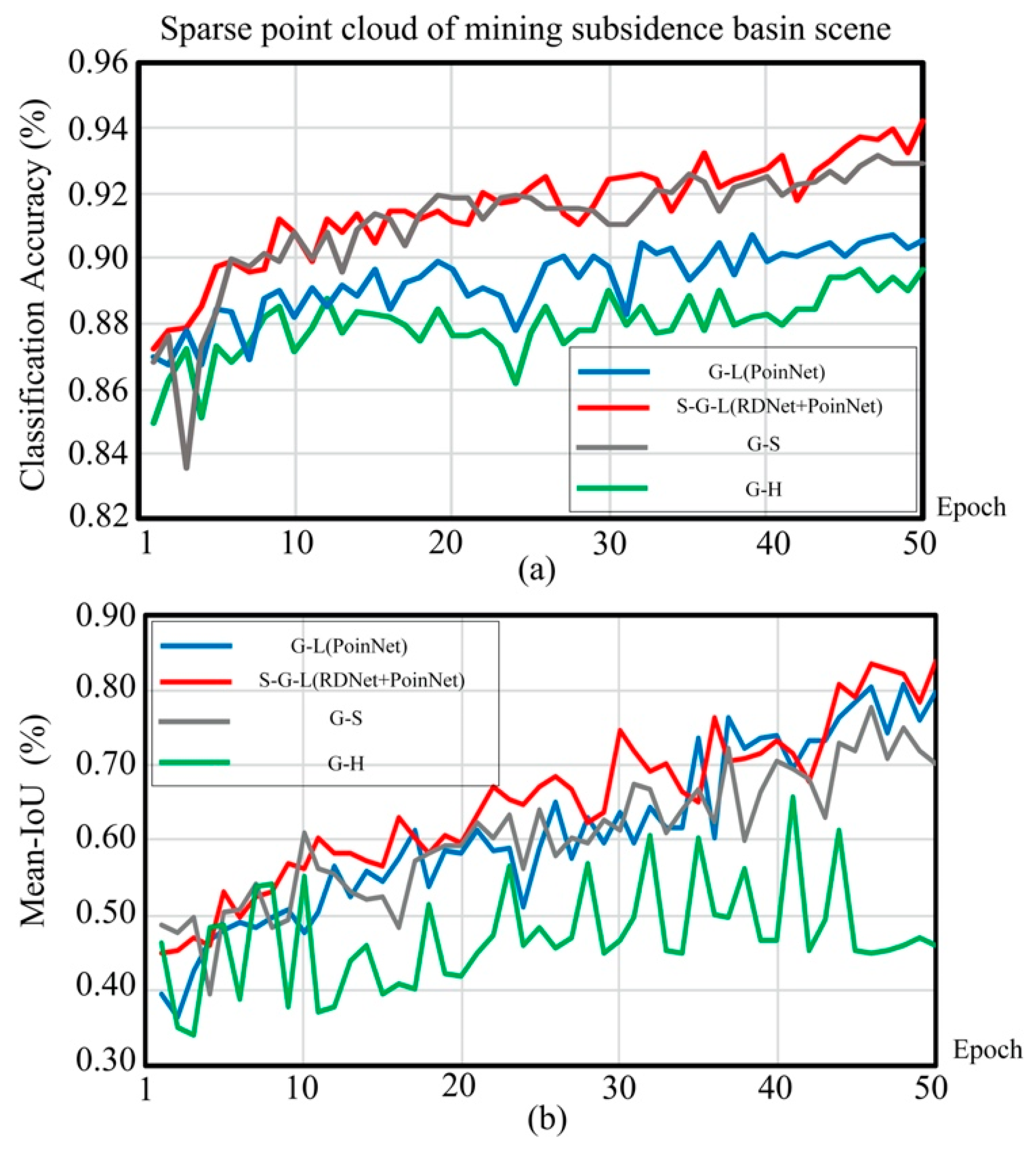
(E1.2) As shown in Table 3 and Figure 13, the S-G-L combination mode performs best among all methods. Compared S-G-L with the G-H method, the S-G-L method increases the classification accuracy by 4.3%. This is because of the optimal utilization of point-density information. Both the G-H and S-G-L methods use point-density and coordinate information. However, the G-H stack the two kinds of information together, for training, while the S-G-L method separates the two kinds of information and uses PointNet to train coordinate information and RD-Net to train the point-density information, independently. This result proves that considering the point-density as independent information instead of the complementary to the coordinate information can significantly improve the performance.

Table 3.
The results of the feature experiment.
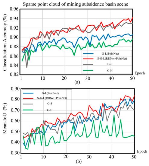
Figure 13.
The results of different feature connected methods for large-scale sparse point cloud. (a) The trend of classification accuracy in 50 epochs. (b) The trend of segmentation mean-IoU in 50 epochs.
Table 3 indicates that the mean-IoU of the G-L is 10% higher than G-S. This phenomenon explains the critical effect of the local feature analysis. Specifically, the local feature represents small-scale local region shapes of objects, which is composed of adjacent points and complement each other. However, the structure feature has a large-scale, which represents the topological relationship of the whole object.
When we use the hybrid feature of small-scale point feature and large-scale point-density feature, the G-H, for segmentation experiments, the mean-IoU is not growth, as shown in Table 3. However, when we use the mixed local feature and the global feature for these experiments, the classification effect still does not grow. This is precise because of the independence of the point-density.
4.2. Results and Discussion on Experiment 2
The selection of radius parameters R in this experiment, is shown in Table 4. As illustrated, the accuracy is impacted by the selection of the radius. For example, when the radius R is selected as 0.2 m, the classification accuracy of the mining subsidence basin is 78.73%. With an increase in R, the classification accuracy improves and reaches the optimal result when R = 2 m. After this, the accuracy decreases as the R increases. This might be because a radius of about 2 meters can express the change of the density distribution of the current point cloud. When the radius is too large, the density range of unit sphere of each point covers the change of point density before and after the rotation of point cloud, vice versa.

Table 4.
Influence of radius parameter R on recognition accuracy of sparse point cloud (mining subsidence basin with RD-Net+PointNet).
4.3. Results and Discussion on Experiment 3
As shown in Table 5, the classification accuracy of sparse point clouds with a small amount of data is slightly lower than that of medium density point clouds, and is slightly higher than dense point clouds with large amounts of data. However, the calculation efficiency is five times that of medium density type and ten times that of high-density type of point cloud. The data size does not significantly impact the classification accuracy when using the RD-Net with coordinate-based network. This phenomenon demonstrated that the point-density information is more sensitive at sparse point cloud, and the proposed method, RD-Net+PointNet, could proficiently process the sparse point cloud with a small amount of file size, which can significantly reduce the computing cost and improve work efficiency. It is of great practical value for studying large-scale surface laws, such as mining subsidence in mining areas.

Table 5.
Comparison with different data size point cloud in terms of both speed and performance, through our proposed method (RD-Net+PointNet).
As displayed in Figure 13, as the point-density of point cloud becomes denser, the gap between the four different feature-combined methods decrease gradually. This result proved that the spatially-local correlation between points increases gradually when the point cloud becomes dense. When the point-density reaches 10 pts/m2, the coordinate has enough spatial information for classification and segmentation and the effect of point-density information is reduced, as in Figure 13. However, a high-density point cloud means a heavy volume of data and longtime calculation.
5. Conclusions
This paper proposed a preprocessing method, GT-Box, to retain spatial information and a novel lightweight network, RD-Net, that can efficiently improve the performance of classification and segmentation in the large-scale sparse point cloud. Specifically, the classification accuracy and the mean-IoU of RD-Net+PointNet are 94.06% and 83.41%. Unlike coordinate-based network, RD-Net does not rely on the coordinates of the point cloud itself when analyzing the point cloud, but through the relative position relationship between the points. The learning parameters of RD-Net and traditional coordinate-based network is independent of each other. Therefore, the two types of networks can complement each other to improve performance. By comparing with the different feature combination connected models in the concatenate layer, we proved that point-density is an independent and scale-sensitive spatial information, and plays an important role in the recognition of sparse point cloud. In addition, comparing the analysis of dense density type of point cloud with large amount of data using our proposed method—RD-Net+PointNet—to classify and segment large-scale sparse point cloud, a similar accuracy could be achieved, but the efficiency was increased ten times. It is practical for geoscientists engaged in regular research, such as mining subsidence. Remarkably, RD-Net+PointNet has a significant improvement effect on large-scale sparse point cloud, but it has little improvement on dense density point cloud. We believe that the reason for this limitation lies in the difficulty in understanding the characteristics of density-sensitive information of point cloud. The recognition of sensitive information features of different densities of point cloud is an exciting future direction, to further improve RD-Net performance.
Author Contributions
Y.Y. and H.Y. designed the experiments; Y.Y. and H.Y. analyzed the data and wrote the paper; H.Y. and J.G. assisted with the process of LiDAR data and labeled the datasets; Y.Y., H.Y., and H.D. assisted in the experimental verification. All authors have read and agreed to the published version of the manuscript.
Funding
This research was funded by National Natural Science Foundation of China, grant number 51404272, 51574242; and State Key Laboratory of Water Resources Protection and Utilization in Coal Mining Independent Research Project, Item Number GJNY-18-77.
Conflicts of Interest
The authors declare no conflict of interest.
References
- Wang, W.; Sakurada, K.; Kawaguchi, N. Reflectance Intensity Assisted Automatic and Accurate Extrinsic Calibration of 3D LiDAR and Panoramic Camera Using a Printed Chessboard. Remote Sens. 2017, 9, 851. [Google Scholar] [CrossRef]
- Błaszczak-Bąk, W.; Suchocki, C.; Janicka, J.; Dumalski, A.; Duchnowski, R.; Sobieraj-Żłobińska, A. Automatic Threat Detection for Historic Buildings in Dark Places Based on the Modified OptD Method. Isprs Int. J. Geo-Inf. 2020, 9, 123. [Google Scholar] [CrossRef]
- Luo, D.A.; Zhu, G.; Lu, L.; Liao, L.Q. Whole Object Deformation Monitoring Based on 3D Laser Scanning Technology. Bull. Surv. Mapp. 2005, 7, 40–42. [Google Scholar]
- Maxwell, A.E.; Warner, T.A.; Strager, M.P.; Conley, J.F.; Sharp, A.L. Assessing machine-learning algorithms and image-and lidar-derived variables for GEOBIA classification of mining and mine reclamation. Int. J. Remote Sens. 2015, 36, 954–978. [Google Scholar] [CrossRef]
- Yang, J.; Jones, T.; Caspersen, J.; He, Y. Object-based canopy gap segmentation and classification: Quantifying the pros and cons of integrating optical and LiDAR data. Remote Sens. 2015, 7, 15917–15932. [Google Scholar] [CrossRef]
- Fu, K.; Dai, W.; Zhang, Y.; Wang, Z.; Yan, M.; Sun, X. MultiCAM: Multiple Class Activation Mapping for Aircraft Recognition in Remote Sensing Images. Remote Sens. 2019, 11, 544. [Google Scholar] [CrossRef]
- Chen, X.; Kohlmeyer, B.; Stroila, M.; Alwar, N.; Wang, R.; Bach, J. Next generation map making: Geo-referenced ground-level LIDAR point clouds for automatic retro-reflective road feature extraction. In Proceedings of the 17th ACM SIGSPATIAL International Conference on Advances in Geographic Information Systems, Chicago, IL, USA, 5–8 November 2019; pp. 488–491. [Google Scholar]
- Wulder, M.A.; Bater, C.W.; Coops, N.C.; Hilker, T.; White, J.C. The role of LiDAR in sustainable forest management. For. Chron. 2008, 84, 807–826. [Google Scholar] [CrossRef]
- Wang, Y.; Chen, Q.; Liu, L.; Li, X.; Sangaiah, A.K.; Li, K. Systematic Comparison of Power Line Classification Methods from ALS and MLS Point Cloud Data. Remote Sens. 2018, 10, 1222. [Google Scholar] [CrossRef]
- Zhao, H.; Qi, X.; Shen, X.; Shi, J.; Jia, J. Icnet for real-time semantic segmentation on high-resolution images. In Proceedings of the European Conference on Computer Vision, Munich, Germany, 8–14 September 2018; pp. 405–420. [Google Scholar]
- Xu, B.; Jiang, W.; Shan, J.; Zhang, J.; Li, L. Investigation on the weighted ransac approaches for building roof plane segmentation from lidar point clouds. Remote Sens. 2016, 8, 5. [Google Scholar] [CrossRef]
- Li, Y.; Bu, R.; Sun, M.; Wu, W.; Di, X.; Chen, B. PointCNN: Convolution on X-Transformed Points. NeurIPS 2018, 828–838. [Google Scholar] [CrossRef]
- LeCun, Y.; Bengio, Y.; Hinton, G. Deep learning. Nature 2015, 521, 436. [Google Scholar] [CrossRef] [PubMed]
- Zou, X.; Cheng, M.; Wang, C.; Xia, Y.; Li, J. Tree Classification in Complex Forest Point Clouds Based on Deep Learning. IEEE Geosci. Remote Sens. Lett. 2017, 14, 2360–2364. [Google Scholar] [CrossRef]
- Jiang, H.; Hu, X.; Li, K.; Zhang, J.; Gong, J.; Zhang, M. PGA-SiamNet: Pyramid Feature-Based Attention-Guided Siamese Network for Remote Sensing Orthoimagery Building Change Detection. Remote Sens. 2020, 12, 484. [Google Scholar] [CrossRef]
- Yang, J.; Kang, Z. Voxel-based extraction of transmission lines from airborne LiDAR point cloud data. IEEE J. Sel. Top. Appl. Earth Obs. Remote Sens. 2018, 11, 3892–3904. [Google Scholar] [CrossRef]
- Heidemann, H.K. Lidar Base Specification (No. 11-B4); US Geological Survey: Reston, VA, USA, 2012.
- Tatebe, Y.; Deguchi, D.; Kawanishi, Y.; Ide, I.; Murase, H.; Sakai, U. Can we detect pedestrians using low-resolution LIDAR? In Proceedings of the Computer Vision Theory and Applications, Porto, Portugal, 27 February–1 March 2017; pp. 157–164. [Google Scholar]
- Tatebe, Y.; Deguchi, D.; Kawanishi, Y.; Ide, I.; Murase, H.; Sakai, U. Pedestrian detection from sparse point-cloud using 3DCNN. In Proceedings of the 2018 International Workshop on Advanced Image Technology (IWAIT), Chiang Mai, Thailand, 7–9 January 2018; pp. 1–4. [Google Scholar]
- Stein, F.; Medioni, G. Structural indexing: Efficient 3-d object recognition. IEEE Trans. Pattern Anal. Mach. Intell. 1992, 14, 125–145. [Google Scholar] [CrossRef]
- Tuzel, O.; Liu, M.-Y.; Taguchi, Y.; Raghunathan, A. Learning to rank 3d features. In Proceedings of the European Conference on Computer Vision, Zurich, Switzerland, 6–12 September 2014; Proceedings, Part I. pp. 520–535. [Google Scholar]
- Gonzalez, A.; Villalonga, G.; Xu, J.; Vazquez, D.; Amores, J.; Lopez, A. Multiview random forest of local experts combining rgb and lidar data for pedestrian detection. IEEE Intell. Veh. Symp. (IV) 2015, 356–361. [Google Scholar] [CrossRef]
- Chen, X.; Kundu, K.; Zhu, Y.; Berneshawi, A.; Ma, H.; Fidler, S.; Urtasun, R. 3d object proposals for accurate object class detection. Adv. Neural Inf. Process. Syst. (Nips) 2015, 424–432. [Google Scholar]
- Song, S.; Xiao, J. Deep Sliding Shapes for amodal 3D object detection in RGB-D images. IEEE Conf. Comput. Vis. Pattern Recognit. (CVPR) 2016, 808–816. [Google Scholar]
- Chen, X.; Ma, H.; Wan, J.; Li, B.; Xia, T. Multi-view 3D Object Detection Network for Autonomous Driving. IEEE Conf. Comput. Vis. Pattern Recognit. (Cvpr) 2017, 6526–6534. [Google Scholar] [CrossRef]
- Charles, R.Q.; Su, H.; Kaichun, M.; Guibas, L.J. PointNet: Deep Learning on Point Sets for 3D Classification and Segmentation. IEEE Conf. Comput. Vis. Pattern Recognit. (Cvpr) 2017, 77–85. [Google Scholar]
- Qi, C.R.; Yi, L.; Su, H.; Guibas, L.J. Pointnet++: Deep hierarchical feature learning on point sets in a metric space. Adv. Neural Inf. Process. Syst. 2017, 5099–5108. [Google Scholar]
- Cheraghian, A.; Rahman, S.; Petersson, L. Zero-shot learning of 3d point cloud objects. Int. Conf. Mach. Vis. Appl. (Mva). IEEE 2019, 1–6. [Google Scholar] [CrossRef]
- Li, J.; Chen, B.M.; Lee, G.H. So-net: Self-organizing network for point cloud analysis. Proc. Ieee Conf. Comput. Vis. Pattern Recognit. 2018, 9397–9406. [Google Scholar]
- Wang, Y.; Sun, Y.; Liu, Z.; Sarma, S.E.; Bronstein, M.M.; Solomon, J.M. Dynamic graph cnn for learning on point clouds. ACM Trans. Graph. (Tog) 2019, 38, 1–12. [Google Scholar] [CrossRef]
- Cheraghian, A.; Rahman, S.; Petersson, L. Zero-shot learning of 3d point cloud objects. In Proceedings of the 2019 16th International Conference on Machine Vision Applications (MVA), Tokyo, Japan, 27–31 May 2019; pp. 1–6. [Google Scholar]
- Riegler, G.; Ulusoy, A.O.; Geiger, A. OctNet: Learning Deep 3D Representations at High Resolutions. Proc. IEEE Conf. Comput. Vis. Pattern Recognit. (CVPR) 2017, 808–816. [Google Scholar] [CrossRef]
- Maturana, D.; Scherer, S. VoxNet: A 3D Convolutional Neural Network for Real-Time Object Recognition. IEEE/Rsj Int. Conf. Intell. Robot. Syst. (IROS) 2015, 922–928. [Google Scholar]
- Zhou, Y.; Tuzel, O. Voxelnet: End-to-end learning for point cloud based 3d object detection. In Proceedings of the IEEE Conference on Computer Vision and Pattern Recognition (CVPR), Salt Lake City, UT, USA, 18–22 June 2018; pp. 4490–4499. [Google Scholar]
- Wang, D.Z.; Posner, I. Voting for voting in online point cloud object detection. Proc. Robot. Sci. Syst. 2015, 1, 10–15607. [Google Scholar]
- Engelcke, M.; Rao, D.; Wang, D.Z.; Tong, C.H.; Posner, I. Vote3deep: Fast object detection in 3d point clouds using efficient convolutional neural networks. IEEE Int. Conf. Robot. Autom. (ICRA) 2017, 1355–1361. [Google Scholar]
- Lang, A.H.; Vora, S.; Caesar, H.; Zhou, L.; Yang, J.; Beijbom, O. Pointpillars: Fast encoders for object detection from point clouds. In Proceedings of the IEEE Conference on Computer Vision and Pattern Recognition (CVPR), Long Beach, CA, USA, 16–20 June 2019; pp. 12697–12705. [Google Scholar]
- Chen, X.; Ma, H.; Wan, J.; Li, B.; Xia, T. Multi-view 3d object detection network for autonomous driving. In Proceedings of the IEEE Conference on Computer Vision and Pattern Recognition (CVPR), Honolulu, HI, USA, 21–26 July 2017; pp. 1907–1915. [Google Scholar]
- Gonzlez, A.; Vzquez, D.; Lpez, A.M.; Amores, J. Onboard object detection: Multicue, multimodal, and multiview random forest of local experts. IEEE Trans. Cybern. 2017, 47, 3980–3990. [Google Scholar] [CrossRef]
- Enzweiler, M.; Gavrila, D.M. A multilevel mixture-ofexperts framework for pedestrian classification. IEEE Trans. Image Process. 2011, 20, 2967–2979. [Google Scholar] [CrossRef]
- Dai, A.; Chang, A.X.; Savva, M.; Halber, M.; Funkhouser, T.; Nießner, M. Scannet: Richly-annotated 3d reconstructions of indoor scenes. In Proceedings of the IEEE Conference on Computer Vision and Pattern Recognition, Honolulu, HI, USA, 21–26 July 2017; pp. 5828–5839. [Google Scholar]
- Pedregosa, F.; Varoquaux, G.; Gramfort, A.; Michel, V.; Thirion, B.; Grisel, O.; Blondel, M.; Prettenhofer, P.; Weiss, R.; Dubourg, V.; et al. Scikit-learn: Machine learning in Python. J. Mach. Learn. Res. 2011, 12, 2825–2830. [Google Scholar]
- Hackel, T.; Savinov, N.; Ladicky, L.; Wegner, J.D.; Schindler, K.; Pollefeys, M. Semantic3d. net: A new large-scale point cloud classification benchmark. arXiv 2017, arXiv:1704.03847. [Google Scholar]
© 2020 by the authors. Licensee MDPI, Basel, Switzerland. This article is an open access article distributed under the terms and conditions of the Creative Commons Attribution (CC BY) license (http://creativecommons.org/licenses/by/4.0/).

