Micro-scale Flood Hazard Assessment Based on Catastrophe Theory and an Integrated 2-D Hydraulic Model: A Case Study of Gongshuangcha Detention Basin in Dongting Lake Area, China

Abstract

Assessments of urban flood hazards are crucial for planning and early warning flood system design. Moreover, hazard risk assessment is useful for emergency planning and insurance. There are two common methods for conducting flood hazard risk assessments (FHRA): those based on physical models and those based on parameters. Although physical models are able to simulate flood propagation processes accurately, they also have obvious shortcomings. Parameter-based FHRAs are more comprehensive because they emphasize the analysis of hazard factors. However, this approach also has various flaws, including its qualitative, macro-scale and high subjective nature. In this study, the strengths of both methods were combined to develop a new micro-scale FHRA. Taking the FHRA of the flood storage and detention area of Dongting Lake as an example, this study used high-precision digital elevation model (DEM) data generated from an airborne light detection and ranging (LiDAR) point cloud to construct a two-dimensional (2-D) flood propagation model. Micro-scale FHRAs were then performed using eight selected FHR indicators based on catastrophe theory. By automatically calculating the FHR value of each assessment unit based on hierarchical recursion, the catastrophe theory and catastrophe progression method effectively avoided uncertainty in weight assignment, which is an issue commonly faced by parameter-based methods. The FHRA results obtained under 144 different sequences of assessment indicators also show that the proposed method has a low sensitivity to the ranking of FHR indicators, as well as a high fault tolerance for different assessment results arising from subjective rankings by humans.

1. Introduction

Flooding can represent a severe natural threat, with large flood events causing substantial casualties and property losses every year [1]. With increased urbanization along riverbanks, alluvial areas are increasingly affected by worsening flooding events in terms of frequency and intensity [2]. Decision makers have used various technical means and assessment methods to formulate flood policies, reduce losses caused by flooding and improve the level of flood hazard management. In the early period of flood hazard research, the focus was on the analysis of flood threats to people; however, more recently, the focus has gradually moved to accurate qualitative and quantitative analyses of disasters, environmental vulnerability and human/material exposures [3].

Three flood hazard risk (FHR) factors—the risk of disaster-causing factors, environmental vulnerability and human/material exposures—have become the cornerstones of current FHR analysis and assessment studies [3]. Many methods for FHR assessment (FHRA) have been proposed. These can be divided into two main categories: (i) traditional FHRA methods based on physical models (PMs) and (ii) parameter-based flood vulnerability assessment methods [4]. The main difference between the two categories is that the former employs PMs to perform FHRAs for specific flood events [5,6,7,8] and can be combined with flood loss assessment models to determine the economic losses in affected areas [9]. The latter uses collectable data to construct assessment indicators on a spatiotemporal scale, and then explores useful information to conduct qualitative assessments of regions’ flood vulnerability. Examples of parameter-based flood vulnerability assessment include the flood vulnerability index (FVI) [10,11], the set pair analysis–variable fuzzy sets (SPA–VFS) model [12], spatial multi-criteria analysis (SMCA) [13]), the block maxima model (BMM) [14] and the decision tree (DT) approach [15].

PM-based FHRAs can accurately simulate the propagation process of a flood event to obtain information including the scope of flood inundation, submerged depth and duration, which are the focal points of FHR research. Digital topographic data are one of the most important data sources for flood simulation research [16]. Multiple studies have shown that high-resolution digital topographies play an important role in improving the accuracy of flood simulations [17,18]. In recent years, the rapid development of light detection and ranging (LiDAR) technologies has greatly facilitated developments in the acquisition and application of high-resolution digital elevation model (DEM) data. Macro-scale, high-resolution DEM data products have become common, which has popularized the application of such data to flood simulation research [19,20,21]. This has provided new opportunities for FHR research, such as micro-scale FHR mapping [22], flood damage assessment for individual buildings [23,24] and micro-scale FHR analysis [25]. The computational complexity of the models used in these studies increases dramatically when their computational grids become more refined. Model design that is more complex requires longer computation time and increases computational instabilities. Balancing the relationship between model complexity and actual application requirements has become a critical research focus [26,27].

Despite the ability of PM-based FHRAs to accurately simulate the propagation process of individual flood events, they are somewhat limited. On one hand, extra emphasis is placed on studying the risk of disaster-causing factors without sufficiently considering the environmental vulnerability and human/material exposures. For FHR parameters, only a few key factors (such as flood submerged depth, flow velocity and duration) are considered for the partitioning of areas based on risk levels to prepare FHR maps. On the other hand, although the characteristic parameters of PM-based FHRAs and the information on disaster-related economic losses can be easily conveyed to and comprehended by the public, the method is dependent on detailed topographic, hydrological and economic data. If there are not so much data available, the results of the FHR analytical method become unverifiable [4].

In contrast, the parameter-based FHRA method is more comprehensive. In addition to considering disaster-causing factors, it concurrently analyzes the environmental vulnerability and human/material exposures, such as population distribution, building vulnerability, DEMs, slope, river and waterway systems and road traffic networks [13,28,29]. The parameter-based FHRA method uses only a small number of attainable flood impact parameters to conduct flood vulnerability assessments of the entire complex system. Unlike PM-based FHRAs, parameter-based FHRAs focus on qualitative evaluation, with many of the applied parameters not having the concepts of spatial distribution or temporal scale. Following from the above, parameter-based FHRAs are usually macro-scale. This is often problematic for policy makers with regard to current trends of refined FHR management. Another issue with parameter-based FHRA methods is that the multiple parameters in the assessment system must each be assigned a certain weight. This is to determine the relative importance of the various types of parameters. Although many studies have introduced ways to assign weights to parameters, such as the analytic hierarchy process [30] and multi-criteria analysis [13], the subjectivity involved cannot be ignored. Weight assignments vary between different users owing to their dissimilar knowledge backgrounds and industry experiences, resulting in different FHRA results.

To address the aforementioned problems, this study fully considered the advantages and disadvantages of both the PM- and parameter-based FHRA methods before proposing a micro-scale FHRA method based on catastrophe theory and with the integration of airborne LiDAR point cloud data and a two-dimensional (2-D) hydraulic model. The Gongshuangcha flood storage and detention area (FSDA) located in China’s Dongting Lake region was selected to test the method. First, airborne LiDAR point cloud data were generated for a high-resolution DEM. Next, a 2-D hydraulic model was used to construct a refined flood propagation model to obtain high-resolution flood simulation results. Spatial discretization of the FHR indicators was conducted by selecting the FHR factors, before comprehensive FHR assessment was performed based on the catastrophe progression method.

2. Study Area and LiDAR Data

2.1. Study Area

Flood storage and detention areas are an important component of river flood control systems that improve safety and mitigate impacts in key areas. These areas require realistic and economical flood control planning, which can become a regional or global consideration requiring compromise and cooperation between many interests. At present, there are 98 major flood storage and detention areas in China, mainly distributed along the middle and lower reaches of the Yangtze, Yellow, Huaihe and Haihe rivers. Although flood peaks and flows are high along the Yangtze River, its channels have insufficient discharge capacity resulting in frequent flooding events throughout recorded history. The Dongting Lake flood storage and detention project is an important component of the basin’s overall flood management.

The Dongting Lake region, located in the middle reaches of the Yangtze River (111°40′–113°10′ E and 28°30′–30°20′ N) and with a total area of 18,780 km², consists of basin-shaped lakes and plains surrounded by mountains. Dongting Lake has an intricate system of feeder drainages distributed in a fan shape, but only one outlet from which the Yangtze River continues downstream. Owing to its special geographical location and complex morphology, this area has always been prone to flooding and requires intense seasonal management. Extensive human, material and financial resources are dedicated on dike management (during winter) and flood control (during summer). There are 266 dikes of different sizes stretching a total of 5812 km; primary and secondary dikes are 3471 and 1509 km long, respectively. However, flood damage in the Dongting Lake area remains severe: direct economic losses in 1996 and 1998 reached 2.14 billion and 1.27 billion US$, respectively. These impacts, along with the heavy repair and protection burden, have significantly limited the area’s socio-economic development.

The Gongshuangcha detention basin is one of 24 large flood storage and detention areas in the Dongting Lake area. Located north of Yanjiang City, it is surrounded by water (Figure 1) and borders the Caowei River to the north, the Huangtubao River to the south, Dongting Lake to the east, and Chishan to the west. The flood detention area covers 293.0 km² (of which cultivated land accounts for 157.6 km²), and the total dike length is 121.74 km. There are three towns in the flood detention area; nearly 164,200 people live here legally. Owing to its large population, the occurrence of a flood disaster would inevitably cause major losses to the local economy, and so it is of great significance to carry out flood hazard evaluations in this area.

2.2. LiDAR Data

A HARRIER 68i airborne laser measurement system from TopoSys (TopoSys GmbH, Biberach, Germany) was used for aerial photography and measurement in the study area. The digital camera in the airborne laser measurement system was a Rollei Metric AIC Pro (60 million pixel) from Trimble (Sunnyvale, CA, USA). The inertial navigation system model was an Applanix POS/AV series with a sampling frequency of 200 Hz. The laser scanner model was a Riegl LMS-Q680i with a maximum pulse frequency of 80–400 kHz and a scanning angle of 45/60°.

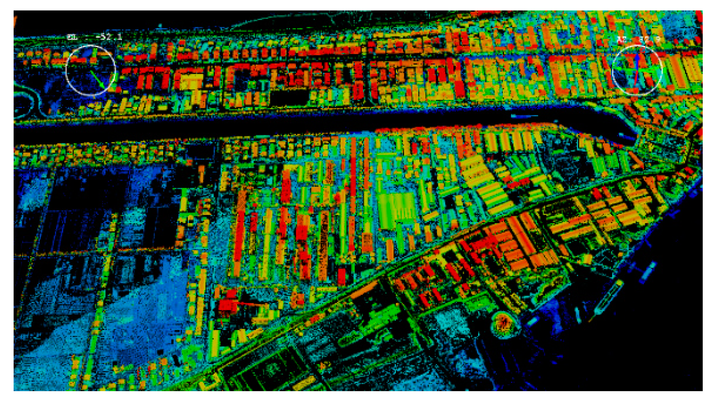
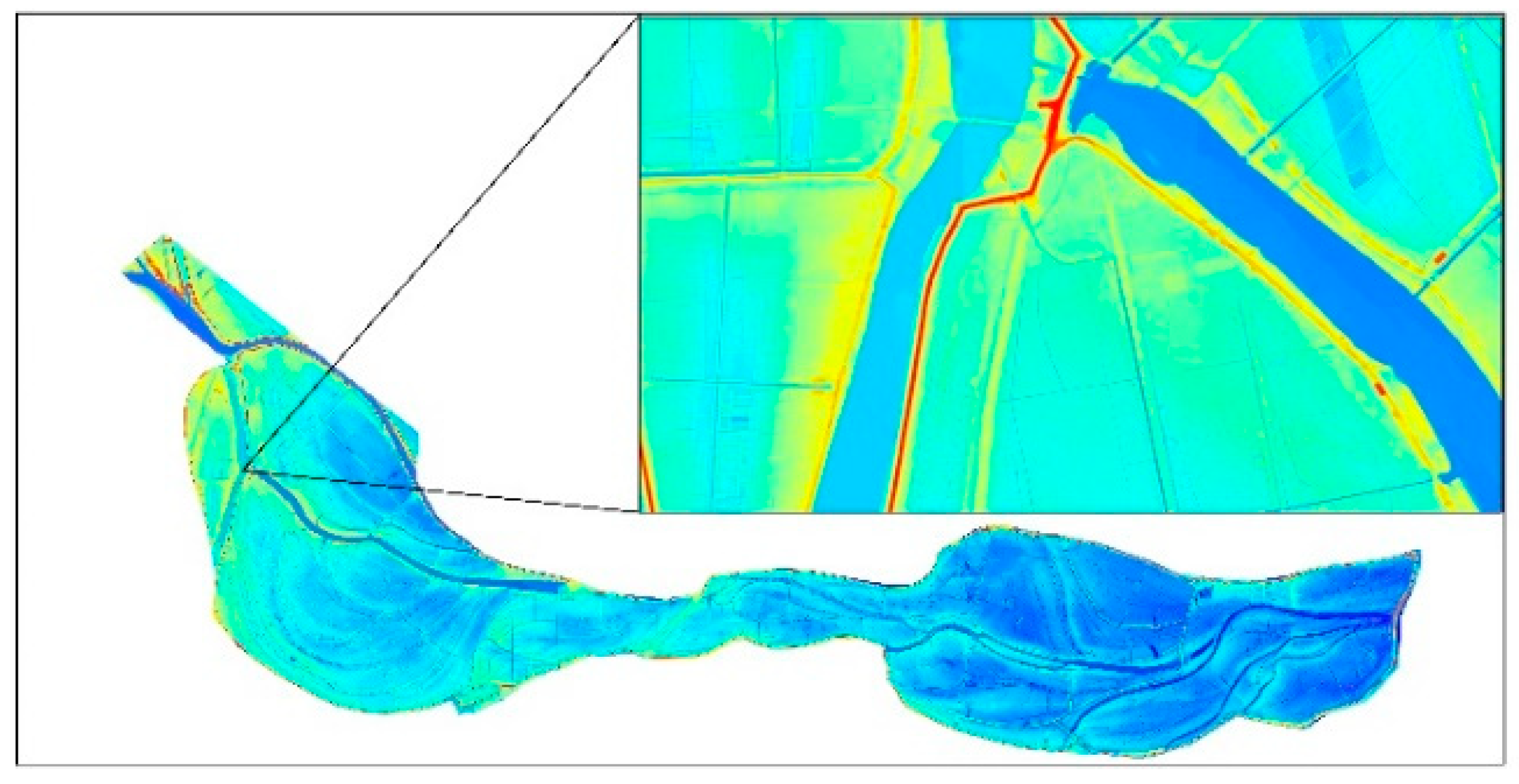
High-resolution DEM data were generated by processing the collected airborne LiDAR point cloud (Figure 2 and Figure 3). The DEM data had a spatial resolution of 1 m and the DEM grid contained 22,000 rows × 51,000 columns. The coordinate system was the Beijing Geodetic Coordinate System 1954 and the height system was the 1985 National Elevation Benchmarks. Seventy control points were selected in field and the average error of the DEM was 0.04 m. The overall terrain was relatively flat, with elevation ranging from 4.55 to 35.09 m. Many microtopographic features such as dikes, ditches and fields were captured by the DEM.

3. Two-dimensional (2-D) Hydraulic Model

The flood routing model used 2-D unsteady flow shallow water equations to describe the water flow. First, based on the natural topography and existing hydraulic structures, the computational area was discretized with an unstructured mesh. Next, the water flow, momentum and concentration balance were established for each mesh unit using the finite volume method in time series to ensure its conservation. The Riemann approximate solution was used to calculate the normal numerical flux of water flow and momentum across the unit to ensure calculation accuracy. The model has three Riemann approximations to be chosen: Osher, flux vector splitting (FVS) and flux-difference splitting (FDS).

The model transformed the 2-D problem into a series of local one-dimensional (1-D) problems by integral discretization of the finite volume method and rotation invariance of flux coordinates using the following calculation principles.

3.1. Basic Control Equation

The vector expression of the conservative 2-D shallow water equation is [31,32]:

$$\frac{\partial \mathrm{q}}{\partial \mathrm{t}}+\frac{\partial \mathrm{f}\left(\mathrm{q}\right)}{\partial \mathrm{x}}+\frac{\partial \mathrm{g}\left(\mathrm{q}\right)}{\partial \mathrm{y}}=\mathrm{b}\left(\mathrm{q}\right),$$

(1)

where, q = [h,hu,hv]T is the conservative physics vector, f(q) = [hu,hu²+gh²/2,huv]T is the flux vector in the x direction and g(q) = [hv,huv,hv²+gh²/2]T is the flux vector in the y direction. Here, h is the water depth; u and v are the vertical mean uniform flow velocity components of the x direction and the y direction, respectively; and g is the acceleration of gravity. The source–sink item b(q) is:

$$\mathrm{b}\left(\mathrm{q}\right)=\left({\mathrm{q}}_{\mathrm{w}},\mathrm{gh}\left({\mathrm{s}}_{0\mathrm{x}}-{\mathrm{s}}_{\mathrm{fx}}\right)+{\mathrm{q}}_{\mathrm{w}}\mathrm{u},\mathrm{gh}\left({\mathrm{s}}_{0\mathrm{y}}-{\mathrm{s}}_{\mathrm{fy}}\right)\right),$$

(2)

where, s_0x and s_fx are the river slope and friction slope in the x direction, respectively; s_0y and s_fy are the river slope and friction slope in the y direction, respectively; q_w is the net rain depth per unit time; and the friction slope in the model is estimated by Manning’s formula.

3.2. Discrete Equations

The divergence theorem was applied to Equation (1) on any unit Ω for integral discretization in order to obtain the basic equation of FVM:

$${{\displaystyle \int }}^{ }{{{\displaystyle \int }}^{ }}_{\mathsf{\Omega }}{\mathrm{q}}_{\mathrm{t}}\mathrm{d}\mathsf{\omega }=-{{{\displaystyle \int }}^{ }}_{\partial \mathsf{\Omega }}\mathrm{F}\left(\mathrm{q}\right)\cdot \mathrm{ndL}+{{\displaystyle \int }}^{ }{{{\displaystyle \int }}^{ }}_{\mathsf{\Omega }}\mathrm{b}\left(\mathrm{q}\right)\mathrm{d}\mathsf{\omega },$$

(3)

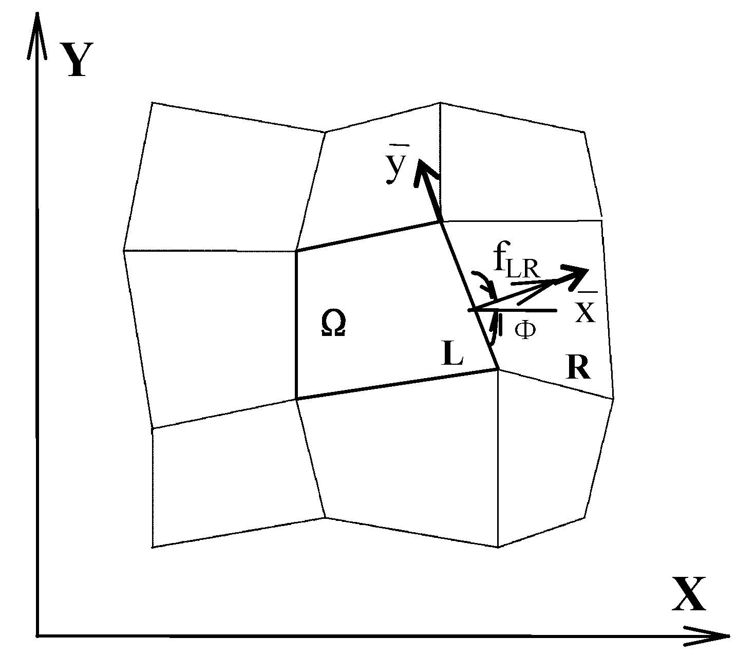
where, n is the normal unit vector; outside unit ∂Ω; dω and dL are the area and line integral infinitesimal elements, respectively; and $\mathrm{F}\left(\mathrm{q}\right)\cdot \mathrm{n}$ is the normal numerical flux. The $\mathrm{F}\left(\mathrm{q}\right)={\left[\mathrm{f}\left(\mathrm{q}\right),\mathrm{g}\left(\mathrm{q}\right)\right]}^{\mathrm{T}}$ shows that the solution of normal flux can transform a 2-D problem into a series of local 1-D problems. The finite volume Ω is shown in Figure 4.

Vector q is the average value of units and to the first order is supposed for the constant. The basic equation of FVM was discretized from Equation (3):

$$\mathrm{A}\frac{\mathrm{dq}}{\mathrm{dt}}=-{{\displaystyle \sum }}_{\mathrm{j}=1}^{\mathrm{m}}{\mathrm{F}}_{\mathrm{n}}^{\mathrm{j}}\left(\mathrm{q}\right){\mathrm{L}}^{\mathrm{j}}+{\mathrm{b}}_{*}\left(\mathrm{q}\right),$$

(4)

where, ${\mathrm{b}}_{*}\left(\mathrm{q}\right)={(\mathrm{A}\cdot {\mathrm{b}}_1,\mathrm{A}\cdot {\mathrm{b}}_2,\mathrm{A}\cdot {\mathrm{b}}_3)}^{\mathrm{T}}$, A is the area of unit $\mathsf{\Omega }$, m is the sum of unit sides, L_j is the length of the j_th side in the unit and b*(q) is the source term. The flux in the direction normal ${\mathrm{F}}_{\mathrm{n}}^{\mathrm{j}}\left(\mathrm{q}\right)$, ${\mathrm{F}}_{\mathrm{n}}\left(\mathrm{q}\right)$ can be defined as follows:

$${\mathrm{F}}_{\mathrm{n}}\left(\mathrm{q}\right)=\cos \mathsf{\Phi }\cdot \mathrm{f}\left(\mathrm{q}\right)+\sin \mathsf{\Phi }\cdot \mathrm{g}\left(\mathrm{q}\right),$$

(5)

The f(q) and g(q) are invariant to rotation and meet the following equation:

$$\mathrm{T}\left(\mathsf{\Phi }\right){\mathrm{F}}_{\mathrm{n}}\left(\mathrm{q}\right)=\mathrm{f}\left[\mathrm{T}\left(\mathsf{\Phi }\right)\mathrm{q}\right]=\mathrm{f}\left(\overline{\mathrm{q}}\right),$$

(6)

and

$${\mathrm{F}}_{\mathrm{n}}\left(\mathrm{q}\right)=\mathrm{T}{(\mathsf{\Phi })}^{-1}\mathrm{f}\left(\overline{\mathrm{q}}\right),$$

(7)

where, $\mathsf{\Phi }$ is the angle between normal vector n and x; and T(Φ) and T(Φ)−1 are the geometrical transform matrix and its inverse matrix, respectively, which are given by:

$$\mathrm{T}\left(\mathsf{\Phi }\right)=\left[\begin{array}{cccc}1& 0& 0& \\ 0& \cos \mathsf{\Phi }& \sin \mathsf{\Phi }& \\ 0& -\sin \mathsf{\Phi }& \cos \mathsf{\Phi }& \\ & & & \end{array}\right];\hspace{1em}\hspace{1em}\mathrm{T}{(\mathsf{\Phi })}^{-1}=\left[\begin{array}{cccc}1& 0& 0& \\ 0& \cos \mathsf{\Phi }& -\sin \mathsf{\Phi }& \\ 0& \sin \mathsf{\Phi }& \cos \mathsf{\Phi }& \\ & & & \end{array}\right],$$

(8)

In turn, this gives:

$$\mathrm{A}\frac{\mathsf{\Delta }\mathrm{q}}{\mathsf{\Delta }\mathrm{t}}=-{{\displaystyle \sum }}_{\mathrm{j}=1}^{\mathrm{m}}\mathrm{T}{(\mathsf{\Phi })}^{-1}\mathrm{f} \left(\overline{\mathrm{q}}\right){\mathrm{L}}^{\mathrm{j}}+{\mathrm{b}}_{*}\left(\mathrm{q}\right),$$

(9)

where, $\overline{\mathrm{q}}$ is transformed from vector q, whose corresponding flow component is in normal and tangential directions. Therefore, the key to solving Equation (9) is $\mathrm{f}\left(\overline{\mathrm{q}}\right)$. Applying the above divergence theorem and flux rotation invariance, the 2-D problem is transformed into a set of normal direction 1-D problems, which can be solved by partial 1-D problems. Since the q of adjacent units can be different, the q value may be discontinuous along boundaries. The Riemann problem was applied in the model to solve $\mathrm{f}\left(\overline{\mathrm{q}}\right)$. The partial 1-D Riemann problem is an initial-value problem:

$${\overline{\mathrm{q}}}_{\mathrm{t}}+{[\mathrm{f}\left(\overline{\mathrm{q}}\right)]}_{\overline{\mathrm{x}}}=0,$$

(10)

which meets

$$\overline{\mathrm{q}}\left(\overline{\mathrm{x}},0\right)=\{\begin{array}{c}{\overline{\mathrm{q}}}_{\mathrm{L}}\hspace{1em}\overline{\mathrm{x}}<0\\ {\overline{\mathrm{q}}}_{\mathrm{R}\hspace{1em}}\overline{\mathrm{x}}>0\end{array},$$

(11)

The origin of $\overline{\mathrm{x}}$ is located at the middle point of unit sides and the direction is in the exterior normal direction. Therefore, $\mathrm{f}\left(\overline{\mathrm{q}}\right)$ is the exterior normal flux at the origin; and ${\overline{\mathrm{q}}}_{\mathrm{L}}$ and ${\overline{\mathrm{q}}}_{\mathrm{R}}$ are the left and right vectors, respectively. Supposing the initial state when t = 0 is known, by solving the Riemann problem we find that the origin is located at $\overline{\mathrm{x}}=0$.

There are three common ways to estimate normal flux $\mathrm{f}\left(\overline{\mathrm{q}}\right)$:

1) Arithmetic average: the average of unit fluxes on both sides of a common border give $\mathrm{f}\left(\overline{\mathrm{q}}\right)$ = [f(${\overline{\mathrm{q}}}_{\mathrm{L}}$)+f(${\overline{\mathrm{q}}}_{\mathrm{R}}$)]/2 or using the average of physically conserved quantities on both sides to calculate the flux as $f\left(\overline{q}\right)$ = f([${\overline{\mathrm{q}}}_{\mathrm{L}}$+${\overline{q}}_R$]/2).

2) Various monotonicity types: examples include total variation descent (TVD) and the flux-corrected transport algorithm (FCT).

3) Riemann approximates based on Eigen theory: flux vector splitting (FVS), flux-difference splitting (FDS) and Osher.

A flood process simulation program was written based on the above model principles. All three estimation approaches were applied in the model for flood coupling solution. The program was able to choose between the three when needed.

3.3. Boundary Conditions

The model determined five types of water flow boundaries: the land boundary, the open boundary of slow and rapid flow, the inner boundary, the dynamic boundary of water exchange and the wetland tributary boundary.

3.4. Equation Solutions

The equations belong to an explicit scheme discretization and are solved by time-interval iteration. According to the ‘Feasibility Study Report on the Flood Diversion and Storage Project of Qianliang Lake, Gongshuangcha and East Dyke of Datonghu in the Dongting Lake Area’ approved by the China Ministry of Water Resources in 2009, during typical flooding events in 1954, 1966 and 1998, when the incoming flood flow in the three flood storage areas was 8000–12,000 m³/s, the water level impact on Chenglingji was minimal. For the 30-year flood in 1954, the study determined that the maximum flood discharge flow of the Gongshuangcha flood diversion sluice was 3630 m³/s and the designed flood discharge water level was 33.10 m.

We simulated the flood routing process by using this sluice to control flood discharge setting its flood discharge hydrograph as the input condition for model calculation. The following conditions were set as follows: when the water level (H) was < 31.63 m, the flow was at the free outflow stage and its rate was 3630 m³/s; when 31.63 < H < 32.60 m, the flow was at the submerged outflow stage and its rate was 3050 m³/s; when 32.60 < H < 33.65 m, a temporary flood diversion sluice was required.

The 2-D hydraulic model mesh was an unstructured triangulation with a total of 83,378 triangular units. Using the 1-m resolution DEM data, nearest-neighbor interpolation was used to obtain the elevation of each triangle apex and center point as the initial condition for model calculation. A flood submerged process of 4 days and 3 hours was simulated, and the flood storage and detention area was eventually completely submerged (Figure 5).

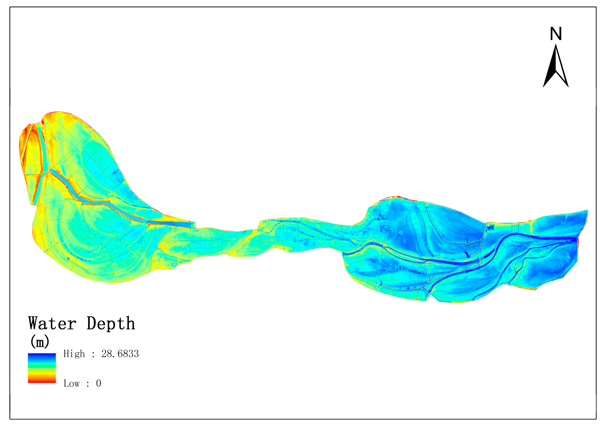
The final completely submerged water depth data (Figure 6) were used for flood risk analysis. The flooding depth in the eastern part of Gongshuangcha was generally deep, while in the west (farther from the inflow sluice) it was relatively shallow.

4. Method Development

4.1. Catastrophe Progression Method

Catastrophe theory, first proposed by Thom [33] and subsequently refined by Zeeman et al. [34], is a mathematical theory to describe the behavior of various non-continuous systems in nature and society. It is mainly used to study the process by which complex systems develop from gradual and quantitative changes to catastrophic and qualitative changes, such as volcanic eruptions, earthquakes and building collapses. Flood events are typical catastrophic processes in the natural environment. The theory assumes that a complex system is controlled by a series of parameters. When the system is in a stable state, the state function used to describe that system should return a unique extreme value, meaning that the state of the system is not affected when the aforementioned parameters change within their respective intervals. If a parameter changes within a certain interval and causes the state function to return more than one extreme value, the system is considered to be unstable. This means that the stability of a system (or the lack thereof) can be determined by observing changes in the extreme value returned by the state function.

The extreme point where the state function is located is where the derivative is zero. Catastrophe theory refers to the point where the derivative of the state function is zero as the critical point and the surface formed by that critical point is known as the equilibrium surface M. It is assumed that the state of a system consists of a combination of multiple unrelated variables with n number of variable combinations ($x1,x2,x3,x4,\dots \dots ,xn$) and that the state function has m number of control parameters ($u1,u2,u3,u4,\dots \dots ,um$). If so, the state function can be expressed as $F_{u1,u2,u3,u4,\dots \dots ,um}(x1,x2,x3,x4,\dots \dots ,xn)$. To get the set of critical points of this state function, the partial differential equation of that function must be solved as follows:

$${\displaystyle \sum _{i=1}^n\frac{d}{d{x}_i}{F}_{u1,u2,u3,u4,\dots \dots ,um}(x1,x2,x3,x4,\dots ,xi,\dots ,xn)=0},$$

(12)

In catastrophe theory, the function $F_{u1,u2,u3,u4,\dots \dots ,um}(x1,x2,x3,x4,\dots \dots ,xn)$ describing the state of the system is the potential function. When studying the stability of a system (or the lack thereof), the issue becomes one of studying the extreme value of the potential function. The variables $x1,x2,x3,x4,\dots \dots ,xn$ describe changes to the system state and are the state variables, while the variables $u1,u2,u3,u4,\dots \dots ,um$ trigger changes to the system’s state and are the control variables. When a control variable changes in a certain region, it will cause sudden changes to the state variables. A set of singularity points S must be identified from the aforementioned set of critical points, where S is a subset of M, which is in turn formed by all the degenerate critical points of F. The set of singularity points not only satisfies Equation (12) but also Equation (13):

$$\Delta \equiv \det \{H(F)\}=0,$$

(13)

where, det represents the determinant and H(F) is the Hessen matrix of F (i.e., the second-order partial derivative matrix of F).

Thom [33] pointed out that many catastrophes in nature can be expressed using particular geometric shapes. A potential function generally does not contain more than four control variables: the natural world is in 3-D and the time dimension is added as the fourth variable. Thom [33] proved that when a potential function contains no more than four control variables, it can at most have seven types of expression that are collectively referred to as the elementary catastrophe types (

Table 1. Seven catastrophe types and their potential functions, x and y are state variables and w, t, u and v are control variables.

Catastrophe Type	No. of Variable(s)		Potential Function
	State	Control
Fold	1	1	$F(x)=x^3+ux$
Cusp	1	2	$F(x)=x^4+u{x}^2+vx$
Swallowtail	1	3	$F(x)=x^5+u{x}^3+v{x}^2+wx$
Butterfly	1	4	$F(x)=x^6+t{x}^4+u{x}^3+v{x}^2+wx$
Hyperbolic umbilic	2	3	$F(x,y)=x^3+x^3+wxy-ux-vy$
Elliptic umbilic	2	3	$F(x,y)=(\frac{1}{3})x^3-x{y}^2+w(x^2+y^2)-ux+vy$
Parabolic umbilic	2	4	$F(x,y)=y^4+x^{2}y+w{x}^2+t{y}^2-ux-vy$

). The first four are the most widely applied in practice because these only consider one state variable.

A multi-objective assessment system often involves more than a dozen (or even dozens of) assessment indicators. With that many indicators, the elementary catastrophe function cannot be applied directly because a maximum of only four control variables are allowed when calculating the state function. At the same time, it is difficult to perfectly rank the importance of the assessment indicators when too many are involved in the calculation. A compromise solution is to place all assessment indicators in a multilevel top-down classification by grouping those indicators that satisfy a particular common characteristic into a small class. Eventually, an inverted hierarchical tree of assessment indicators is constructed. The initial assessment indicators are located at the leaf nodes of the tree structure, with each parent node having a maximum of four child nodes. The relationship between the parent and child nodes can be regarded as that between the state and control variables under catastrophe theory. The different values of the control variables affect the value of the state variables; the effect of the former on the latter can be either large or small. It is for this reason that catastrophe theory is suitable for multi-objective assessments. During specific applications, the actual meanings of the assessment indicators differ, as do their dimensions and value ranges. To facilitate the calculation of the elementary catastrophe model, it is necessary to first normalize the values of the various indicators [35].

(1) Fold catastrophe

There is only one control variable in a fold catastrophe and so it can be directly normalized to the range of [0,1] according to the value range of the control variable.

(2) Cusp catastrophe

In a cusp catastrophe, the value range of x is limited to [0,1]. At this time, the function of x for u and v becomes:

$$\{\begin{array}{l}x=\sqrt{u}\\ x=\sqrt[3]{v}\end{array},$$

(14)

(3) Swallowtail catastrophe

By the same principle, a swallowtail catastrophe is normalized to obtain:

$$\{\begin{array}{l}x=\sqrt{u}\\ x=\sqrt[3]{v}\\ x=\sqrt[4]{w}\end{array},$$

(15)

(4) Butterfly catastrophe

Normalization of the butterfly catastrophe gives:

$$\{\begin{array}{l}x=\sqrt{t}\\ x=\sqrt[3]{u}\\ x=\sqrt[4]{v}\\ x=\sqrt[5]{w}\end{array},$$

(16)

The normalization equation is also known as the fuzzy membership function. The open root mean square situation of the control and state variables indicates that the impacts of the former on the latter vary. In a cusp catastrophe, the control variable x is more important than v; in a swallowtail catastrophe, u > v > w; and in a butterfly catastrophe, t > u > v > w. The various elementary catastrophe types can be determined according to the relationship between the parent and child nodes on the tree structure. Starting from the leaf nodes at the bottommost layer, the catastrophe level is calculated step by step until the value of the comprehensive assessment indicator at the topmost level is reached. When there is mutual impact among the various child nodes in the same parent–child node, the average value of the catastrophe level is adopted when it is passed up to the next level. If such a mutually-constraining relationship does not exist, then the minimum value is adopted according to catastrophe theory, meaning that the minimum value of the catastrophe level is passed to the parent node. At present, catastrophe theory has been widely applied in the field of ecological environments, including assessing island ecological environments [36], sustainable use of urban water resources [37] and risks of water pollution [38].

4.2. Selection and Normalization of FHR Indicators

It is critical to carefully consider the FHR factors and their interrelationships [39]. There are definite differences in the FHR factors affecting different regions, such that a factor with significant impacts on a certain region may not be as important elsewhere [40]. For the Dongting Lake region, FHR-related factors representative of the three aspects (the risk of disaster-causing factors, environmental vulnerability and human/material exposures) were selected according to the region’s characteristics and by making full use of previously accumulated remotely sensed geographic information and socioeconomic data. The three key indicators for the dangers of the disaster-causing factors included the maximum submerged depth, maximum flow velocity and flood submergence duration. The four indicators for environmental vulnerability were the DEMs, ditches, river systems and road networks. For the human/material exposures, the main indicator considered was the flood vulnerability of buildings. In this study, the 1-m DEM grid was used as the basic assessment unit for conducting micro-scale FHRAs. The selection of comprehensive FHR indicators is shown in Figure 7 and are described in detail below.

(1) Maximum Submerged Depth

Flood submerged depth, flow velocity and duration are the three most important FHR indicators. Some PM-based FHRA methods directly generate FHR maps using submerged depth values [6]. In this study, the calculation results of the flood propagation model were interpolated to the DEM grid according to the inverse distance weighted algorithm [41]. After interpolation, the maximum submerged depth of each assessment unit was calculated to generate the overall maximum submerged depth map of the study area, as shown in Figure 8a. The flood submerged depth was generally 4–6 m.

(2) Maximum Flow Velocity

The results of the flood propagation model were interpolated to obtain the maximum flow velocity of each assessment unit. The generated maximum flow velocity map of the study area is shown in Figure 8b, with the values being 0–2.51 m/s.

(3) Flood Submergence Duration

The flood submergence duration map of the study area is shown in Figure 8c and the values were 0–98.8 h. The map was generated by interpolating the results of the flood propagation model to obtain the flood submergence duration of each assessment unit.

(4) DEM

Ground elevation, which is sensitive to FHR and is an important factor for FHR analysis [42], was directly acquired through DEM data. The DEM generated from the LiDAR cloud data of the study area was directly used as the assessment indicator to generate the ground elevation map, as shown in Figure 8d. The elevations of the study area varied from 4.55 to 35.09 m.

(5) Ditches

Ditches refer to furrows, irrigation channels and other wading structures set up between pieces of farmland. Floodwaters entering the FSDAs will flow through these ditches. When ditches overflow, flooding will occur on farmlands and residential lands, posing a risk to surrounding areas. The method proposed by Qian et al. [43] was used to directly generate data on ditches in the study area from the high-resolution DEM. The raster distance map of ditches, as shown in Figure 8e, was generated according to the principle that the closer an area is to a ditch, the higher the risk in that area. The raster distances of ditches were 0–262 m.

(6) River Systems

To a certain extent, the river and waterway systems reflect the precipitation and underlying surface conditions of a region, and are strongly related to FHR. Places with densely populated river systems, high precipitation and weak permeability face relatively higher FHRs [44]. Tehrany et al. [45] generated buffers zones at various distances from rivers to characterize FHR levels while Xiao et al. [30] and Chen et al. [46] used raster distances to characterize the FHRs of rivers. Two rivers flow through the study area. After entering the FSDA, floodwaters advance along the river channels and overflow the banks on both sides, posing a risk to the surrounding areas. Proximity to the river channels was deemed to be directly proportional to FHRs. This principle was used to generate the raster distance map of river systems for the entire study area, as shown in Figure 8f. The raster distances for the river systems were 0–6471.19 m.

(7) Road Networks

There is a road traffic network within the FSDA, as well as diversion roads built on the surrounding dikes. When floods occur, an effective way to avoid the hazard is to make use of roads for diversion and evacuation. The principle of proximity to roads being inversely proportional to FHR level was used to generate the raster distance map of road networks, as shown in Figure 8g. The raster distances from the diversion roads were 0–3204.61 m.

(8) Buildings

A total of 33,930 buildings were extracted from the study area’s airborne LiDAR point cloud using the method for analyzing 3-D fractal dimensions [47]. Of these, 3379 buildings were misclassified and manually eliminated, leaving 30,551 buildings in the study area. The accuracy rate was 90.04% [24]. Buildings are vulnerable to flood hazards and their risk levels are related to the building type, replacement cost and submerged depth. Considering the generality of comprehensive FHRAs, the FHR of buildings were simplified to only take into account their locations. Assuming that proximity to a building equals greater FHR, the raster distance map of buildings was generated and shown in Figure 8h. The raster distances were 0–657.86 m.

For comprehensive assessment of the FHR level, it is first necessary to measure individual FHR indicators (i.e., to grade them). This study set five FHR levels: mini, light, medium, heavy and extreme, represented by the Roman numerals I, II, III, IV and V, respectively. The comprehensive FHR was divided into [0, 1] intervals; the ranges of the five levels were expressed as [0, 0.2], [0.2, 0.4], [0.4, 0.6], [0.6, 0.8] and [0.8, 1.0], respectively. These quantified the various FHR levels. Quantile classification is commonly used to categorize FHR indicators [15]. Considering the characteristics of such indicators, adjustments were made to the value range of each indicator specified under the various FHR levels. At the same time, each FHR indicator has various dimensions and needs to be normalized [30]. The eight normalized FHR indicators are shown in

Table 2. Normalization of flood hazard risk (FHR) indicators.

FHR Level		I	II	III	IV	V	Notes for Indicator Values
	Indicator values	[0, 0.2]	[0.2, 0.4]	[0.4, 0.6]	[0.6, 0.8]	[0.8, 1.0]
(1)	Maximum flood submerged depth	0.0–0.5	0.5–1.5	1.5–3.0	3–5	5–8	If > 8 m, = 1
(2)	Maximum flow velocity	0.0–0.3	0.3–0.7	0.7–1.2	1.2–1.8	1.8–2.5	If > 2.5 m/s, = 1
(3)	Flood submergence duration	0–12	12–24	24–48	48–72	72–120	If > 120 h, = 1
(4)	DEM	60–40	40–20	20–10	10–5	5–0	If > 60 m, = 0
(5)	Ditches	300–200	200–150	150–100	100–50	50–0	If > 300 m, = 0
(6)	River systems	1000–800	800–600	600–400	400–200	200–0	If > 1000 m, = 0
(7)	Road networks	0–800	800–1600	1600–2400	2400–200	3200–4000	If > 4000 m, = 1
(8)	Buildings	1000–800	800–600	600–00	400–200	200–0	If > 1000 m, = 0

.

4.3. Calculating Catastrophe Level Based on FHR Indicators

(1) Disaster-Causing Factors

Figure 7 shows that the main indicators constituting the disaster-causing factors were the maximum submerged depth, maximum flow velocity and flood submergence duration. These three control variables affected the state variable of disaster-causing factors. The latter was a typical swallowtail catastrophe and satisfied the normalized form of Equation (15).

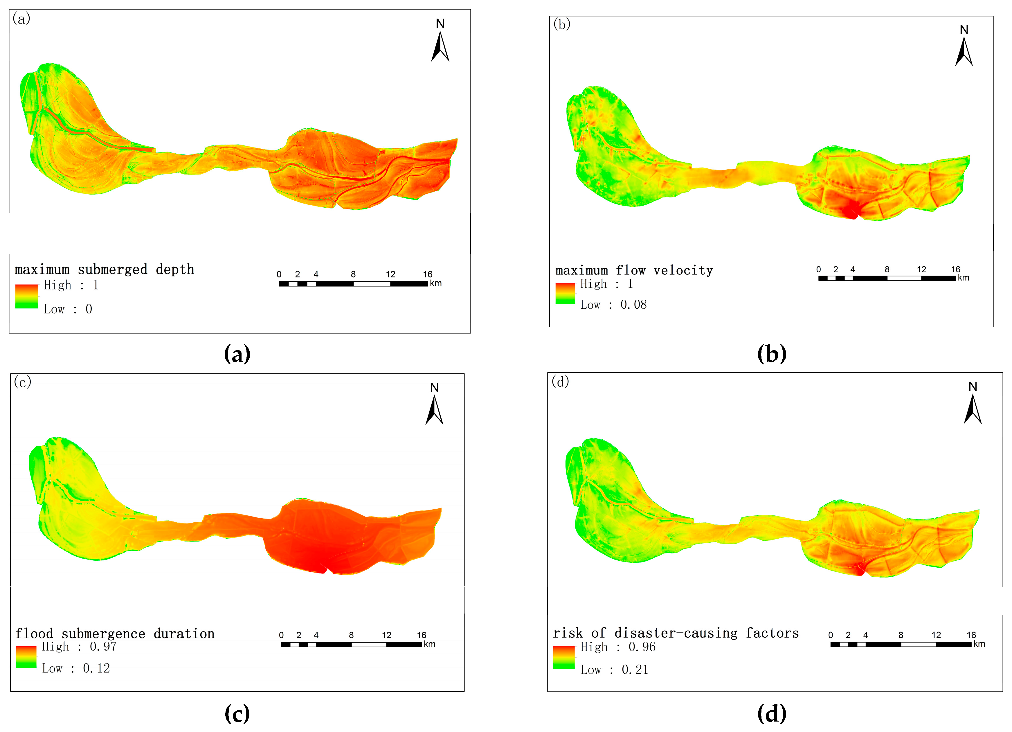
The normalized Equation (15) for swallowtail catastrophes was used to obtain the square root of the normalized value of the maximum submerged depth. This gave the swallowtail catastrophe value for the maximum submerged depth, as shown in Figure 9a. The cube root of the normalized value of the maximum flow velocity gave the swallowtail catastrophe value for the latter, as shown in Figure 9b. The swallowtail catastrophe value for the flood submergence duration was obtained by taking root four of its normalized value, as shown in Figure 9c. Since there are strong correlations among these three FHR indicators, the catastrophe theory principle of determining the value was applied. Specifically, the mean of the swallowtail catastrophe value of the three indicators was used as the risk value of the disaster-causing factors, meaning that $B1=\left(\sqrt{C1}+\sqrt[3]{C2}+\sqrt[4]{C3}\right)/3$. A map of the risk of disaster-causing factors is shown in Figure 9d.

(2) Environmental Vulnerability

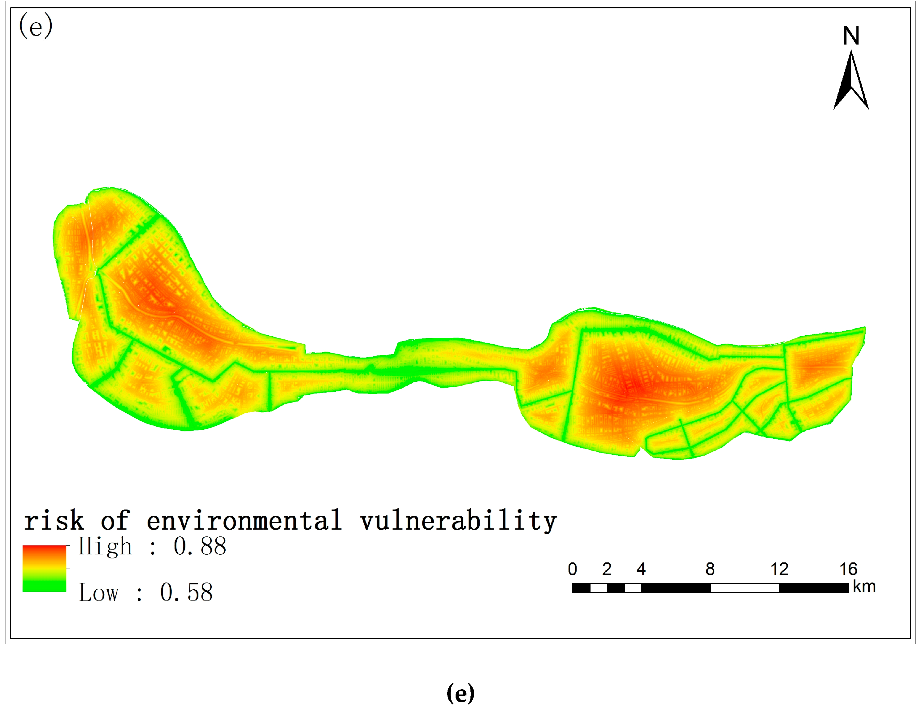
Similarly, Figure 7 shows that the main indicators that constituted environmental vulnerability were ground elevation, ditches, river systems and road networks. These four control variables affected the state variable of environmental vulnerability. They satisfied the normalized form of Equation (16) for butterfly catastrophes; Equation (16) was used to obtain the square root of the normalized value of the ground elevation to obtain its butterfly catastrophe value as shown in Figure 10a. The cube root of the normalized value of the ditches gave its butterfly catastrophe value as shown in Figure 10b. The butterfly catastrophe values for the river systems and road networks were obtained by taking the roots four and five of their respective normalized values. The results are shown in Figure 10c,d, respectively.

The catastrophe theory’s principle of determining value was applied again because of the strong correlations among the four FHR indicators. Specifically, the mean of the butterfly catastrophe values of the four indicators was used as the risk value of the environmental vulnerability; that is, $B2=\left(\sqrt{C4}+\sqrt[3]{C5}+\sqrt[4]{C6}+\sqrt[5]{C7}\right)/4$. A map showing the risk of environmental vulnerability is shown in Figure 10e.

(3) Human/Material Exposures

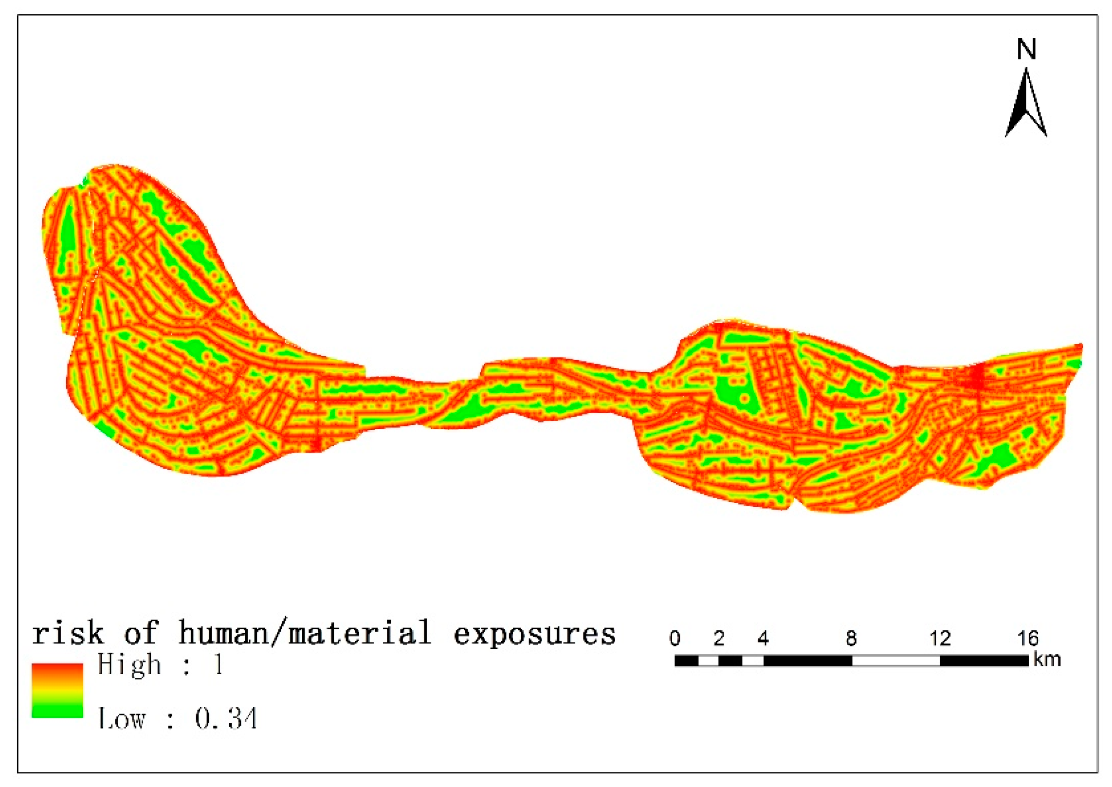
The main indicator for the human/material exposures was buildings (Figure 7). The latter is the only control variable affecting the former as a state variable and is typical of a fold catastrophe. According to the catastrophe progression method, the value of the control variable of the fold catastrophe can be directly assigned to its state variable. Therefore, the FHR map for the vulnerability of human/material exposures was the same as that for the normalized indicator value of buildings (Figure 11).

4.4. Generation of Comprehensive FHR Maps

For each assessment unit in the study area, the risk values of the disaster-causing factors, environmental vulnerability and human/material exposures were obtained based on the rules for assessing the catastrophe level and according to the bottom-up progression approach. These three types of indicator values constitute a swallowtail catastrophe. This meant that the disaster-causing factors, environmental vulnerability and human/material exposures were the control variables, whereas the comprehensive FHR was the state variable. This satisfies the calculation conditions of Equation (15) for swallowtail catastrophes.

The normalized Equation (15) for swallowtail catastrophes was used to obtain the square root of the normalized value of the disaster-causing factors, which gave the latter’s swallowtail catastrophe value, as shown in Figure 12a. The cube root of the normalized value of the environmental vulnerability gives its swallowtail catastrophe value, as shown in Figure 12b. Taking root four of the normalized value of the human/material exposures gives its swallowtail catastrophe value, as shown in Figure 12c.

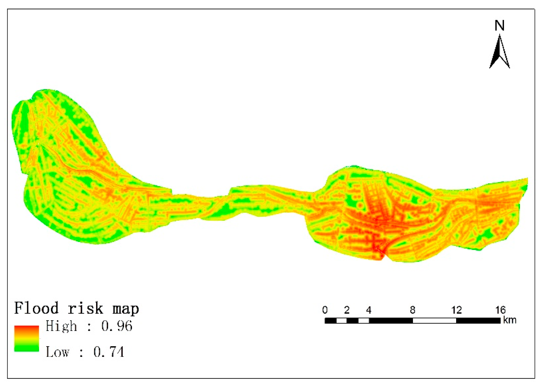
Considering the correlations among the three control variables, the catastrophe theory principle of determining value was applied; that is, the mean of the swallowtail catastrophe values of the three indicators was used as the risk value of the comprehensive FHR. As such, $A=\left(\sqrt{B1}+\sqrt[3]{B2}+\sqrt[4]{B3}\right)/3$. A generated comprehensive FHR map is shown in Figure 13.

5. Discussion

The study area was categorized under level IV and V risks based on the 1954 flood type of the Yangtze River. Areas with higher FHRs were mainly distributed in the east, representing the first region to be flooded. In terms of the flood submerged depth, flow velocity and submergence duration, values in the eastern region were all higher than those in the western region. According to the catastrophe progression method, this study ranked disaster-causing factors ahead of environmental vulnerability and human/material exposures because it was significantly more important. Overall, the three types of disaster-causing factors, namely flood submerged depth, flow velocity and submergence duration, had a greater proportion of impact on the indicator design.

A comparison of Figure 12c and Figure 13 reveals that the risk of human/material exposures represented by buildings is also well reflected in the FHR map. In Figure 9d, which is the risk map considering disaster-causing factors only, some areas in the western region are still at mild and moderate risks (levels II and III). However, the FHR of areas with buildings greatly increased after superpositioning the risk of human/material exposures, as shown on Figure 9d. After environmental vulnerability was integrated into the map, the study area became devoid of areas with mild and moderate risks.

In commonly used parameter-based FHRAs, the assignment of weights to the FHR indicators must be carefully considered to avoid human influence. Taking the analytic hierarchy process (AHP) as an example [30], accurate evaluations must be made of the consistency index (CI), random consistency index (RI) and coefficient of reliability (CR). It is generally believed that CR < 0.1 for passing the consistency test, which indicates that the weight design is ideal. Otherwise, the weights of the indicators need to be re-adjusted. The catastrophe progression method avoids the complicated issue of weight design. When classifying the risk indicators from top to bottom, the evaluators are only required to sort the various indicators under the same node according to their relative importance. Once the hierarchy tree for the FHR indicators has been established, the comprehensive FHR can be automatically calculated. This way, the impact of human factors in the catastrophe progression method is mainly reflected in the ranking of the importance of the various FHR indicators by different evaluators.

To this end, this study analyzed the impact of the comprehensive FHR based on the ranking of the FHR indicators. There were eight indicator types (C1, C2, C3, C4, C5, C6, C7 and C8), of which C1, C2 and C3 belong to the same category, C4, C5, C6 and C7 belonged to another category and C8 is an independent category. C1–C3 and C4–C7 were separately rearranged and recombined, meaning that the former had $P_3^3=3!=6$ permutations and combinations and the latter, $P_4^4=4!=24$ permutations and combinations. If the order of B1, B2 and B3 was unchanged, there would be 6 × 24 × 1 = 144 permutations and combinations for C1–C8. The catastrophe progression method was used to calculate the comprehensive FHR for those 144 permutations and combinations.

The comprehensive FHR results based on the indicators ranked according to C1, C2, C3, C4, C5, C6, C7 and C8 was used as the baseline; the other 143 FHR results were compared with the baseline results. Assuming that the baseline FHR value of each assessment unit was V_cell, then the maximum and minimum assessment values of the other 143 FHR results would be V_cellmax and V_cellmin, respectively. This means that the maximum percentage increase and reduction of an assessment unit would be (V_cellmax − V_cell)/V_cell0 and |(V_cell0 − V_cellmin)|/V_cell0, respectively. Next, the comprehensive FHR value of each assessment unit was compared with the maximum percentage increase and reduction of the baseline value. The statistical results are shown in Figure 14.

The comparative charts indicate that the deviations from the baseline value were minor regardless of the maximum percentage increase or reduction. Among the 143 calculation results for the entire study area, deviations of the maximum percentage increase and reduction from the baseline value were 0.524%–2.89% and 2.12%–6.45%, respectively. For the map of the maximum percentage increase, areas with greater variations were mostly located in the western region. As this region’s FHR values were relatively low in the baseline assessment results, the magnitude of change under the different permutations and combinations was greater. For the map of the maximum percentage reduction, areas with greater variations were mostly located along the diversion roads. This means that under the different permutations and combinations, the roads indicator had a greater impact.

The study area had a total of 6,008,678 assessment grids. For each assessment grid, the number of grid under the maximum percentage increase and reduction was calculated to generate the histograms shown in Figure 15. The histograms for the maximum percentage increase were mainly distributed in the 0.8%–1.3% region. The mean was 1.14% and the standard deviation was 0.12%. The histograms for the maximum percentage reduction were mainly distributed in the 3.15%–5% region, with the mean and standard deviation being 4.19% and 0.39%, respectively.

The above analysis indicates that the catastrophe progression method is not sensitive to changes in ranking of the importance of FHR indicators arising from human factors and that the fault tolerance of the final FHRA results are high. The normalization and grading of individual indicators and factors were the two processes with the greatest impacts on the FHRA results. This being the case, the expert scoring method can be applied to both processes to ensure the soundness and universal acceptance of the FHR value of the individual factors.

Only vulnerability of buildings was selected as one index of the human/material exposures, a lot of further research can be done. Different building structures have different impact on flood resistance. The buildings in the study area are mainly divided into two types: brick-concrete structure and brick-wood structure, which have different flood loss rate curve [24]. Building indicator then can be further divided into two categories to express different risk levels, for example, the risk of brick-wood structure is greater than that of brick-concrete structure. In addition, economic and industrial factors can also be considered as human/material exposures. For different villages, their economical and industrial development level can be normalized into the assessment grid.

6. Conclusions

FHR maps are usually calculated using administrative areas (such as townships and villages) as the basic FHRA units. The limitations of the assessment unit mean that the various calculation indicators for the same assessment unit must be assigned a similar value, which simplifies the FHR indicator values to some extent. However, during practical application, many assessment indicators are spatially related. The most representative examples are river and waterway systems and diversion roads. Although the network density of these two features within an administrative area can be used to characterize the respective indicator values for the assessment unit, changes in the network form are still not being considered. For example, when a river traverses multiple assessment units, it will be artificially segmented. It is unrealistic for the indicator value (such as the flood submerged depth) to be evenly distributed among the assessment units because there are spatial variations to that value. Typically, the mean flood submerged depth of the entire assessment unit is adopted to match the scale of the unit.

This study attempted to place the assessment unit of comprehensive FHRAs on a micro-scale by using a 1-m grid as the basic assessment unit. This was equivalent to performing independent calculation processes for the catastrophe level of every 1-m grid unit. In doing so, the spatial changes of different assessment indicators (such as the flood submerged depth) are better reflected. Those indicators related to spatial location (such as buildings) are also better expressed and analyzed. When these indicators are used in studies with administrative areas as the assessment units, they often have to be simplified values that do not consider spatial locations and are dimensionless, such as building density [48]. The proposed micro-scale FHRA method can provide more detailed results than the classical flood hazard map.

The catastrophe progression method automatically executes hierarchical recursive calculations. Once the level that an FHR indicator is determined and the individual indicators are normalized, the calculation results of the catastrophe progression method are always unique. Both the normalization of individual indicators and the calculation of comprehensive FHR values follow the basic idea of catastrophe theory: a state variable has two stable extreme values (the maximum and minimum values), with all values in between being unstable states. The calculation process shows that the catastrophe progression method effectively avoids the subjective issues faced by common FHRAs, specifically, weight assignment to the various FHR indicators. In contrast, the catastrophe progression method only needs to consider the level of importance of each type of FHR indicator. This results shows that the important indicators should be placed ahead of the secondary indicators. This approach is more intuitive and easier to grasp than assigning weights to the various indicators.

The research shows that micro-scale FHRAs can be realized by integrating airborne LiDAR point cloud data and a 2-D hydraulic model. Catastrophe theory and the catastrophe progression method automatically calculated the FHR value of each assessment grid based on hierarchical recursion, thereby effectively avoiding the problem of uncertainty in weight assignment faced by the common parameter-based methods. The FHRA results for 144 different sequences of assessment indicators show that the proposed method has low sensitivity to the ranking of FHR indicators and high fault tolerance of different assessment results arising from subjective rankings by humans.

References

1. Opolot, E. Application of remote sensing and geographical information systems in flood management: A review. Res. J. Appl. Sci. Eng. Techol. 2013, 6, 1884–1894. [Google Scholar] [CrossRef]
2. Bronstert, A. Floods and climate change: Interactions and impacts. Risk Anal. 2003, 23, 545–557. [Google Scholar] [CrossRef] [PubMed]
3. Birkholz, S.; Muro, M.; Jeffrey, P.; Smith, H.M. Rethinking the relationship between flood risk perception and flood management. Sci. Total Environ. 2014, 478, 12–20. [Google Scholar] [CrossRef] [PubMed]
4. Balica, S.F.; Popescu, I.; Beevers, L.; Wright, N.G. Parametric and physically based modelling techniques for flood risk and vulnerability assessment: A comparison. Environ. Model. Softw. 2013, 41, 84–92. [Google Scholar] [CrossRef]
5. Kalyanapu, A.J.; Judi, D.R.; McPherson, T.N.; Burian, S.J. Mote Carlo-based flood modelling framework for estimating probability weighted flood risk. J. Flood Risk Manag. 2012, 5, 37–48. [Google Scholar] [CrossRef]
6. Masood, M.; Takeuchi, K. Assessment of flood hazard, vulnerability and risk of mid-eastern Dhaka using DEM and 1D hydrodynamic model. Nat. Hazards 2012, 61, 757–770. [Google Scholar] [CrossRef]
7. Falter, D.; Vorogushyn, S.; Lhomme, J.; Apel, H.; Gouldby, B.; Merz, B. Hydraulic model evaluation for large-scale flood risk assessments. Hydrol. Process. 2013, 27, 1331–1340. [Google Scholar] [CrossRef] [Green Version]
8. Schober, B.; Hauer, C.; Habersack, H. A novel assessment of the role of Danuhe floodplains in flood hazard reduction (FEM method). Nat. Hazards 2015, 75, 33–50. [Google Scholar] [CrossRef]
9. Samantaray, D.; Chatterjee, C.; Singh, R.; Gupta, P.K.; Panigrahy, S. Flood risk modeling for optimal rice planning for delta region of Mahanadi river basin in India. Nat. Hazards 2015, 76, 347–372. [Google Scholar] [CrossRef]
10. Balica, S.F.; Douben, N.; Wright, N.G. Flood vulnerability indices at varying spatial scales. Water Sci. Technol. J. 2009, 60, 2571–2580. [Google Scholar] [CrossRef]
11. Balica, S.F.; Wright, N.G. Reducing the complexity of flood vulnerability index. Environ. Hazard J. 2010, 9, 321–339. [Google Scholar] [CrossRef]
12. Zou, Q.; Zhou, J.; Zhou, C.; Song, L.; Guo, J. Comprehensive flood risk assessment based on set pair analysis-bariable fuzzy sets model and fuzzy AHP. Stoch. Environ. Res. Risk Assess. 2013, 27, 525–546. [Google Scholar] [CrossRef]
13. Wang, Y.; Li, Z.; Tang, Z.; Zeng, G. A GIS-based spatial multi-criteria approach for flood risk assessment in the dongting lake region, hunan, central China. Water Resour. Manag. 2011, 25, 3465–3484. [Google Scholar] [CrossRef]
14. Lei, X.; Qiao, Z.; Zhou, A.; Huo, R. Assessment of flood catastrophe risk for grain production at the provincial scale in China based on the BMM method. J. Integr. Agric. 2013, 12, 2310–2320. [Google Scholar]
15. Tehrany, M.S.; Pradhan, B.; Jebur, M.N. Spatial prediction of flood susceptible areas using rule based decision tree (DT) and a novel ensemble bivariate and multivariate statistical models in GIS. J. Hydrol. 2013, 504, 69–79. [Google Scholar] [CrossRef]
16. Garrote, L.; Bras, R.L. A distributed model for real-time flood forecasting using digital elevation models. J. Hydrol. 1995, 167, 279–306. [Google Scholar] [CrossRef] [Green Version]
17. Raber, G.T.; Jensen, J.R.; Hodgson, M.E.; Tullis, J.A.; Davis, B.A.; Berglund, J. Impact of lidar nominal post-spacing on DEM accuracy and flood zone delineation. Photogramm. Eng. Remote Sens. 2007, 73, 793–804. [Google Scholar] [CrossRef] [Green Version]
18. Sanders, B.F. Evaluation of on-line DEMs for flood inundation modeling. Adv. Water Resour. 2007, 30, 1831–1843. [Google Scholar] [CrossRef]
19. Fewtrell, T.J.; Duncan, A.; Sampson, C.C.; Neal, J.C.; Bates, P.D. Benchmarking urban flood models of varying complexity and scale using high resolution terrestrial LiDAR data. Phys. Chem. Earth 2011, 36, 281–291. [Google Scholar] [CrossRef]
20. Sampson, C.C.; Fewtrell, T.J.; Duncan, A.; Shaad, K.; Horrit, M.S.; Bates, P.D. Use of terrestrial laser data to drive decimetric resolution urban inundation models. Adv. Water Resour. 2012, 14, 1–17. [Google Scholar] [CrossRef]
21. Meesuk, V.; Vojinovic, Z.; Mynett, A.E.; Abdullah, A.F. Urban flood modelling combining top-view LiDAR data with ground-view SfM observations. Adv. Water Resour. 2015, 75, 105–117. [Google Scholar] [CrossRef]
22. Webster, T.L. Flood risk mapping using LiDAR for annapolis royal, nova scotia, Canada. Remote Sens. 2010, 2, 2060–2082. [Google Scholar] [CrossRef] [Green Version]
23. Mongkonkerd, S.; Hirunsalee, S.; Kanegae, H.; Denpaiboon, C. Comparison of direct monetary flood damage in 2011 to pillar house and non-pillar house in Ayutthaya, Thailand. Procedia Environ. Sci. 2013, 17, 327–336. [Google Scholar] [CrossRef] [Green Version]
24. Shen, D.; Qian, T.; Chen, W.; Chi, Y.; Wang, J. A quantitative flood-related building damage evaluation method using airborne LiDAR data and 2-D hydraulic model. Water 2019, 11, 987. [Google Scholar] [CrossRef] [Green Version]
25. Ernst, J.; Dewals, B.J.; Detrembleur, D.S.; Archambeau, P.; Erpicum, S.; Pirotton, M. Micro-scale flood rsik analysis based on detailed 2D hydraulic modeling and high resolution geographic data. Nat. Hazards 2010, 55, 181–209. [Google Scholar] [CrossRef]
26. Dottori, F.; Di Baldassarre, G.; Todini, E. Detailed data is welcome, but with a pinch of salt: Accuracy, precision, and uncertainty in flood inundation modeling. Water Resour. Res. 2013, 49, 6079–6085. [Google Scholar] [CrossRef]
27. Costabile, P.; Macchione, F. Enhancing river model set-up for 2-D dynamic flood modelling. Environ. Model. Softw. 2015, 67, 89–107. [Google Scholar] [CrossRef]
28. Chen, H.; Ito, Y.; Sawamukai, M.; Tokunaga, T. Flood hazard assessment in the kujukuri plain of chiba prefecture, Japan, based on GIS and multicriteria decision analysis. Nat. Hazards 2015, 78, 105–120. [Google Scholar] [CrossRef]
29. Papaioannou, G.; Vasiliades, L.; Loukas, A. Multi-criteria analysis framework for potential flood prone areas mapping. Water Resour. Manag. 2015, 29, 399–418. [Google Scholar] [CrossRef]
30. Xiao, Y.; Yi, S.; Tang, Z. Integrated flood hazard assessment based on spatial ordered weighted averaging method considering spatial heterogeneity of risk preference. Sci. Total Environ. 2017, 599–600, 1034–1046. [Google Scholar] [CrossRef]
31. Liang, Q.; Borthwick, A.G.L. Adaptive quadtree simulation of shallow flows with wet–dry fronts over complex topography. Comput. Fluids 2009, 38, 221–234. [Google Scholar] [CrossRef]
32. Wang, Y.; Liang, Q.; Kresserwani, G.; Hall, J.W. A 2D shallow flow model for practical dam-break simulations. J. Hydraul. Res. 2011, 49, 307–316. [Google Scholar] [CrossRef]
33. Thom, R. Catastrophe Theory: Its present state and future perspectives. In Dynamical Systems-Warwick 1974; Springer: Berlin/Heidelberg, Germany, 1975. [Google Scholar]
34. Zeeman, E.C. Catastrophe Theory: Selected Papers (1972~1977); Addson-Wesley: Boston, MA, USA, 1977. [Google Scholar]
35. Lai, C.; Chen, X.; Chen, X.; Wang, Z.; Wu, X.; Zhao, S. A fuzzy comprehensive evaluation model for flood risk based on the combination weight of game theory. Nat. Hazards 2015, 77, 1243–1259. [Google Scholar] [CrossRef]
36. Gao, S.; Sun, H.; Zhao, L.; Wang, R.; Xu, M.; Cao, G. Dynamic assenssment of island ecological environment sustainability under urbanization based on rough set, synthetic index and catastrophy progression analysis theories. Ocean Coast. Manag. 2019, 178, 104790. [Google Scholar] [CrossRef]
37. Chen, Y.; Zhang, S.; Zhang, Y.; Liu, L.; Qu, Z.; Song, G.; Zhang, J. Comprehensive assessment and hierarchical management of the sustainable utilization of urban water resources based on catastrophe theory. J. Taiwan Inst. Chem. Eng. 2016, 60, 430–437. [Google Scholar] [CrossRef]
38. Wang, W.; Liu, S.; Zhang, S.; Chen, J. Assessment of a model of pollution disaster in near-shore coastal waters based on catastrophe theory. Ecol. Model. 2011, 222, 307–312. [Google Scholar] [CrossRef]
39. Liu, Y.B.; De Smedt, F. Flood modeling for complex terrain using GIS and remote sensed information. Water Resour. Manag. 2005, 19, 605–624. [Google Scholar] [CrossRef]
40. Kia, M.B.; Pirasteh, S.; Pradhan, B.; Mahmud, A.R.; Sulaiman, W.N.A.; Moradi, A. An artificial neural network model for flood simulation using GIS: Johor River Basin, Malaysia. Environ. Earth Sci. 2012, 67, 251–264. [Google Scholar] [CrossRef]
41. Shen, D.; Wang, J.; Cheng, X.; Rui, Y.; Ye, S. Integration of 2-D hydraulic model and high-resolution lidar-derived DEM for floodplain flow modeling. Hydrol. Earth Syst. Sci. 2015, 19, 3605–3616. [Google Scholar] [CrossRef] [Green Version]
42. Pradhan, B. Flood susceptible mapping and risk area delineation using logistic regression, GIS and remote sensing. J. Spat. Hydrol. 2010, 9, 1–18. [Google Scholar]
43. Qian, T.; Shen, D.; Xi, C.; Chen, J.; Wang, J. Extracting Farmland Features from Lidar-Derived DEM for Improving Flood Plain Delineation. Water 2018, 10, 252. [Google Scholar] [CrossRef] [Green Version]
44. Glenn, E.; Morino, K.; Nagler, P.; Murray, R.; Pearlstein, S.; Hultine, K. Roles of saltcedar (Tamarix spp.) and capillary rise in salinizing a non-flooding terrace on a flow-regulated desert river. J. Arid Environ. 2012, 79, 56–65. [Google Scholar] [CrossRef]
45. Tehrany, M.S.; Pradhan, B.; Jebur, M.N. Flood susceptibility mapping using a novel ensemble weights-of-evidence and support vector machine medels in GIS. J. Hydrol. 2014, 512, 332–343. [Google Scholar] [CrossRef]
46. Chen, Y.; Liu, R.; Barrett, D.; Gao, L.; Zhou, M.; Renzullo, L.; Emelyanova, I. A Spatial assessment framework for evaluating flood risk under extreme climates. Sci. Total Environ. 2015, 538, 512–523. [Google Scholar] [CrossRef]
47. Yang, H.; Chen, W.; Qian, T.; Shen, D.; Wang, J. The extraction of vegetation points from LiDAR using 3D fractal dimension analyses. Remote Sens. 2015, 7, 10815–10831. [Google Scholar] [CrossRef] [Green Version]
48. Silva, S.F.; Martinho, M.; Capitao, R.; Reis, T.; Fortes, C.J.; Ferreira, J.C. An index-based method for coastal-flood risk assenssment in low-lying area (Costa de Caparica, Portugal). Ocean Coast. Manag. 2017, 144, 90–104. [Google Scholar] [CrossRef]
Figure 1. Location of the Gongshuangcha detention basin in the Dongting Lake area.
Ijgi 09 00206 g001
Figure 2. Example of airborne light detection and ranging (LiDAR) point cloud data.
Ijgi 09 00206 g002
Figure 3. Example of high-resolution digital elevation model (DEM) data.
Ijgi 09 00206 g003
Figure 4. Finite volume Ω, where x ¯ is left side of the boundary, y ¯ is right side of the boundary, f LR is flux and Φ is the angle in the normal direction of the boundary.
Ijgi 09 00206 g004
Figure 5. Two-dimensional (2-D) hydraulic model calculation result (water elevation in m).
Ijgi 09 00206 g005
Figure 6. Calculated flood depth.
Ijgi 09 00206 g006
Figure 7. Selection tree of comprehensive flood hazard risk (FHR) indicators.
Ijgi 09 00206 g007
Figure 8. Maps of various flood hazard risk (FHR) indicators. (a) maximum flood submerged depth, (b) maximum flow velocity, (c) flood submergence duration, (d) digital elevation model (DEM), (e) raster distances of ditches, (f) raster distances of river systems, (g) raster distances of road networks and (h) raster distances of buildings.
Ijgi 09 00206 g008
Figure 9. Swallowtail catastrophe calculations for the disaster-causing factors. (a) swallowtail catastrophe of the maximum submerged depth, (b) swallowtail catastrophe of the maximum flow velocity, (c) swallowtail catastrophe of the flood submergence duration and (d) risk of disaster-causing factors.
Ijgi 09 00206 g009
Figure 10. Butterfly catastrophe calculations for environmental vulnerability. (a) Butterfly catastrophe of ground elevation, (b) butterfly catastrophe of ditches, (c) butterfly catastrophe of river systems, (d) butterfly catastrophe of road networks and (e) risk of environmental vulnerability.
Ijgi 09 00206 g010aIjgi 09 00206 g010bIjgi 09 00206 g010c
Figure 11. Vulnerability risk map of human/material exposures.
Ijgi 09 00206 g011
Figure 12. Swallowtail catastrophe calculation map for the comprehensive flood hazard risk (FHR). (a) disaster-causing factors, (b) environmental vulnerability and (c) human/material exposures.
Ijgi 09 00206 g012
Figure 13. Comprehensive flood hazard risk (FHR) map.
Ijgi 09 00206 g013
Figure 14. Ranking map of flood hazard risk (FHR) indicators and the impact map on assessment results. (a) maximum percentage increase and (b) maximum percentage reduction.
Ijgi 09 00206 g014
Figure 15. Histograms for the (a) maximum percentage increase and (b) maximum percentage reduction.
Ijgi 09 00206 g015