Unfolding Events in Space and Time: Geospatial Insights into COVID-19 Diffusion in Washington State during the Initial Stage of the Outbreak

Abstract

The world witnessed the COVID-19 pandemic in 2020. The first case of COVID-19 in the United States of America (USA) was confirmed on 21 January 2020, in Snohomish County in Washington State (WA). Following this, a rapid explosion of COVID-19 cases was observed throughout WA and the USA. Lack of access to publicly available spatial data at finer scales has prevented scientists from implementing spatial analytical techniques to gain insights into the spread of COVID-19. Datasets were available only as counts at county levels. The spatial response to COVID-19 using coarse-scale publicly available datasets was limited to web mapping applications and dashboards to visualize infected cases from state to county levels only. This research approaches data availability issues by creating proxy datasets for COVID-19 using publicly available news articles. Further, these proxy datasets are used to perform spatial analyses to unfolding events in space and time and to gain insights into the spread of COVID-19 in WA during the initial stage of the outbreak. Spatial analysis of theses proxy datasets from 21 January to 23 March 2020, suggests the presence of a clear space–time pattern. From 21 January to 6 March, a strong presence of community spread of COVID-19 is observed only in close proximity of the outbreak source in Snohomish and King Counties, which are neighbors. Infections diffused to farther locations only after a month, i.e., 6 March. The space–time pattern of diffusion observed in this study suggests that implementing strict social distancing measures during the initial stage in infected locations can drastically help curb the spread to distant locations.

1. Introduction

The world has witnessed several epidemics and pandemics throughout history, few being very recent. The World Health Organization (WHO) provides a list of such pandemics and epidemic diseases [1]. In 2019, the WHO reported that pneumonia of unknown cause was detected in Wuhan, China, on 31 December 2019 [2]. This pneumonia, caused by a virus, was referred to as the “2019 novel coronavirus” until WHO announced “COVID-19” as the official name for the virus [3]. The virus is thought to spread from person to person, between people within 6 feet of close contact or through contact with respiratory droplets produced by an infected person [4]. Within a matter of days, COVID-19 had reached different continents, after which the WHO characterized it as a pandemic [5]. In the initial stage, COVID-19 spread from China to other countries, such as South Korea, Italy, Iran, and Japan, which were among the worst hit, with multiple reported cases of COVID-19 infections and fatalities [6]. The first confirmed case in the United States of America (USA) was reported on 21 January 2020, in Snohomish County of Washington State (WA) [7]. In the following discussion, this case is referred to as patient zero, who had returned to the USA after traveling for a family visit to Wuhan, China. In the following days, multiple cases were detected not only in WA State but also all over the US [8]. In WA State, there were 132 deaths and 2580 confirmed positive cases by 25 March 2020 [9].

As the author writes this manuscript on 26 March 2020, the world is struggling to contain the COVID-19 pandemic. Figure 1 shows the status of worldwide confirmed cases of COVID-19 as of 26 March 2020. Testing kits are available only to detect COVID-19 infection. However, no medication or vaccine is available to treat or cure infections. Given this scenario, the only immediate option is to implement social distancing strategies in order to slow and reduce the spread from person to person. Social distancing strategies can range from maintaining a 6-foot distance to implementing complete lockdowns. However, the comparative effectiveness of these strategies is not known. It can be assumed that a complete lockdown will result in a maximum rate of slowing the spread of infection. It was reported that emergency measures, although disrupting day-to-day life, have been effective in slowing the spread of COVID-19 in WA [10]. Similar aggressive social distancing strategies have worked in some other countries, such as China [11].

As a response to the COVID-19 pandemic, Johns Hopkins University, WHO, and several other organizations developed interactive web-based GIS dashboards to visualize and track globally reported cases in real-time [12,14]. Boulos and Geraghty [15] provide an overview of GIS and mapping dashboards that were developed for mapping the near real-time spread of COVID-19. These dashboards obtain data from a variety of open-source authoritative platforms that publish and update COVID-19 cases frequently. For the USA, these dashboards display information such as the number of confirmed cases, deaths, and recovered and active cases at the county level. Unfortunately, these dashboards do not provide detailed information and provide little to no use in locating and analyzing the space–time dynamics of COVID-19 at a detailed spatial resolution, i.e., large-scale areas. Given this, unfortunately, these dashboards serve as no more than a source of an impressive visualization tool for mapping COVID-19 in real-time. Washington State Department of Health (WSDH) created its own database and dashboard to display similar information at county levels [9]. However, on 25 March, WSDH announced (see Figure 2) that, “The state’s notifiable conditions database is currently experiencing a slowdown because of a 10-fold increase in the number of lab reports received. Our IT team is working to correct the issue”. With an increase in the number of confirmed positive cases and a slowdown in the updating of databases, these dashboards face difficulties updating in real-time. In the USA, as of 26 March 2020, the finest resolution of publicly available data for COVID-19 is the county level [16]. This, too, is not a fine enough scale to understand where and when COVID-19 spread. Sizes of counties can vary; a case identified in a county could be located anywhere within that county. This non-availability of data can be tied closely to three issues: first, maintaining the privacy of patients; second, avoiding panic amongst populations who live close to these COVID-19 cases; third, the lack of opportunity to create a detailed inventory of infected cases because of the prevalence of a huge number of cases.

As of 26 March 2020, the pandemic has become so out of control at such a large scale that there is a need to move beyond dashboards. While medical intervention such as preventive vaccines and curative medicines that work are being considered [17], methods that are currently effective in slowing the spread include quarantine, isolation, and mass lockdown of not only infected and close contact individuals but entire populations. The repercussions include fears of economic slowdown, another recession, job insecurity, and so on [18]. The question then is, how and when can spatial analysis help? The answer to this is not only to understand how COVID-19 is spreading but also, more importantly, to know where and when it spreads from patient zero during the initial stage so that appropriate social distancing measures can be implemented immediately in affected locations. Insights into COVID-19 spread within immediately neighboring communities and from one location to another can help in planning mitigation and preventive actions. China has implemented a dedicated app for detecting close contact between individuals and a person confirmed or suspected to have a COVID-19 infection [15]. However, such a strategy is not permissible in the USA because of privacy concerns. At least some academics have raised opinions regarding this situation [19]. The use of geospatial analysis for epidemiology is not new [20]; hence, analyzing geospatial datasets for COVID-19 is an obvious way forward. GIS can aid in mapping, tracing, modeling, and forecasting a phenomenon. An important question is, given the advances in geospatial science technologies, why has no one yet moved beyond dashboards to map and analyze the space–time spread of COVID-19? The availability of accurate, precise, and timely location information for conducting a geospatial analysis of health-related studies is a recurring challenge [21]. The COVID-19 data availability situation is no different. Unfortunately, detailed levels of datasets are not publicly available for GIS researchers who can utilize this opportunity. The unavailability of data at spatial scales finer than the county level causes difficulties in utilizing the strength of geospatial technologies that can map and analyze the spread in space–time, thus gaining meaningful insights. With this in mind, this research seeks three objectives. The first goal is to create proxy geospatial datasets at a fine resolution by locating cases of COVID-19 in WA during the initial stage by referring to local and national online news articles. The second objective is to use these datasets to map the spread of COVID-19 in space and time. The third aim is to gain insights into where, when, and how COVID-19 spread during the initial stage in WA. Analyzing where and when COVID-19 cases spread from patient zero’s location to other locations and determining how long it took for new cases to appear in distant locations can provide insights into where and when timely social distancing strategies could have been implemented in affected areas to reduce the spread. This is the first study that uses online news articles to retrieve geospatial information for COVID-19 analysis in WA. To the best of the author’s knowledge, no other study has applied the foregoing approach to locate, map, and analyze the space–time spread of COVID-19 in WA at a finer spatial scale.

2. Materials and Methods

2.1. Study Area

This research focuses on WA as the study area. WA is part of the Pacific Northwest region, with the North Pacific Ocean to the west. The Cascade Mountain range divides the state into two contrasting sides, Western and Eastern WA. Western WA is located on the windward side of the Cascades and hence exhibits a temperate climate and is damp during most months of the year; it is sometimes referred to as the “wet side”. Eastern WA is in the rain shadow of the Cascades and hence has a relatively dry climate with semiarid steppes and is therefore sometimes known as the “dry side” (see Figure 3). Approximately 77% of the total state’s population is present in Western WA. Some of the major cities and towns are located in three counties in Western WA—King, Pierce, and Snohomish—and are concentrated on the western side of those counties. Seattle, Bellevue, Kent, Renton, and Federal Way are located in King County, Tacoma is located in Pierce County, and Everett is in Snohomish County. The economy of the state is strong because of the presence of multiple fortune 500 companies. Some of the leading companies, such as Amazon, Costco, Microsoft, Starbucks, Paccar, Nordstrom, Expedia, Alaska Air group, Weyerhaeuser, and Expedia, are located in King County itself. This has attracted a diverse population to the area. It is common for people working in these companies to live in Snohomish or Pierce County, bordering King County towards the north and south, or in King County itself. Major highways, such as I-5, I-90, and I-405, provide good connectivity between these three counties. Besides this, the presence of a strong public transportation system, which includes Everett Transit, King County Metro, Sound Transit, and Spokane Transit Authority, amongst others, provides convenient mobility opportunities to travel between work and home for the majority of the population in these urban areas. The presence of interstate and state highways, as well as the nation’s largest ferry system, provides good connectivity between all counties within the state. The foregoing description of the study area provides the necessary background for the analyses and discussion in the following sections.

The author is familiar with the study area, having lived in Seattle and traveled throughout WA. Since February 2020, the author started receiving multiple local news article suggestions on the phone and other digital devices regarding COVID-19 in WA. In the initial stage of the outbreak, local news articles were reporting details of new cases of COVID-19 that were detected in WA. As the author read through multiple news pieces, it was comprehended that these articles with public information were a vital source that could be used to locate, map, and analyze the spread of COVID-19 in WA during the initial stage. For this reason, WA was chosen as the study area. This research focuses on the potential for retrieving geospatial data from local news articles and using these datasets to visualize, analyze and gain insights into when, where, and how COVID-19 spread in WA during the initial stage. The following section discusses the data creation process.

2.2. Data Collection

During the initial stage of the COVID-19 outbreak in WA, local online news articles were reporting details of every new COVDI-19-positive case. Note that these cases refer to people who were tested and confirmed positive. News articles from different sources, such as KOMO, KING, KIRO, Seattle Times, and Q13 News, were used. Reported case details varied among articles. In general, the information included a patient’s age, gender, county name, local place name or work location, history of international or local travel, the hospital admitted to, date of testing positive for COVID-19, exposure to COVID-19 and infection level status. The author manually scanned multiple digital articles and derived the place names and attributes of each case by cross-checking it with different news articles. The same case information reported in different news articles was reported only once in the database to avoid duplication. Data were collected for cases reported from 21 January 2020 to 23 March 2020. In this timeframe, news articles were reporting new cases identified in other counties, along with additional information. As the number of cases increased, the information reported for each case became less detailed. Unfortunately, case-by-case news was no longer reported because of the drastic increase in the number of infected cases. Nonetheless, for this research, in order to analyze space–time spread dynamics, the most important data needed were place names and the dates of testing positive.

With this approach, a total of 100 cases were identified; however, three of these cases did not have any place name or location information, and hence, they were excluded from the dataset. Finally, a total of 97 cases were included in this study. Next, the place name of each case was converted to latitude and longitude coordinates. A customized program was developed in Python for automating the process of obtaining latitude and longitude coordinates from place-names. In doing that, the place name of each case was obtained from the database, and a search query was performed using Google Maps in the Chrome browser, which returned the latitude and longitude coordinates. These latitude and longitude coordinates were used as proxy locations in this study.

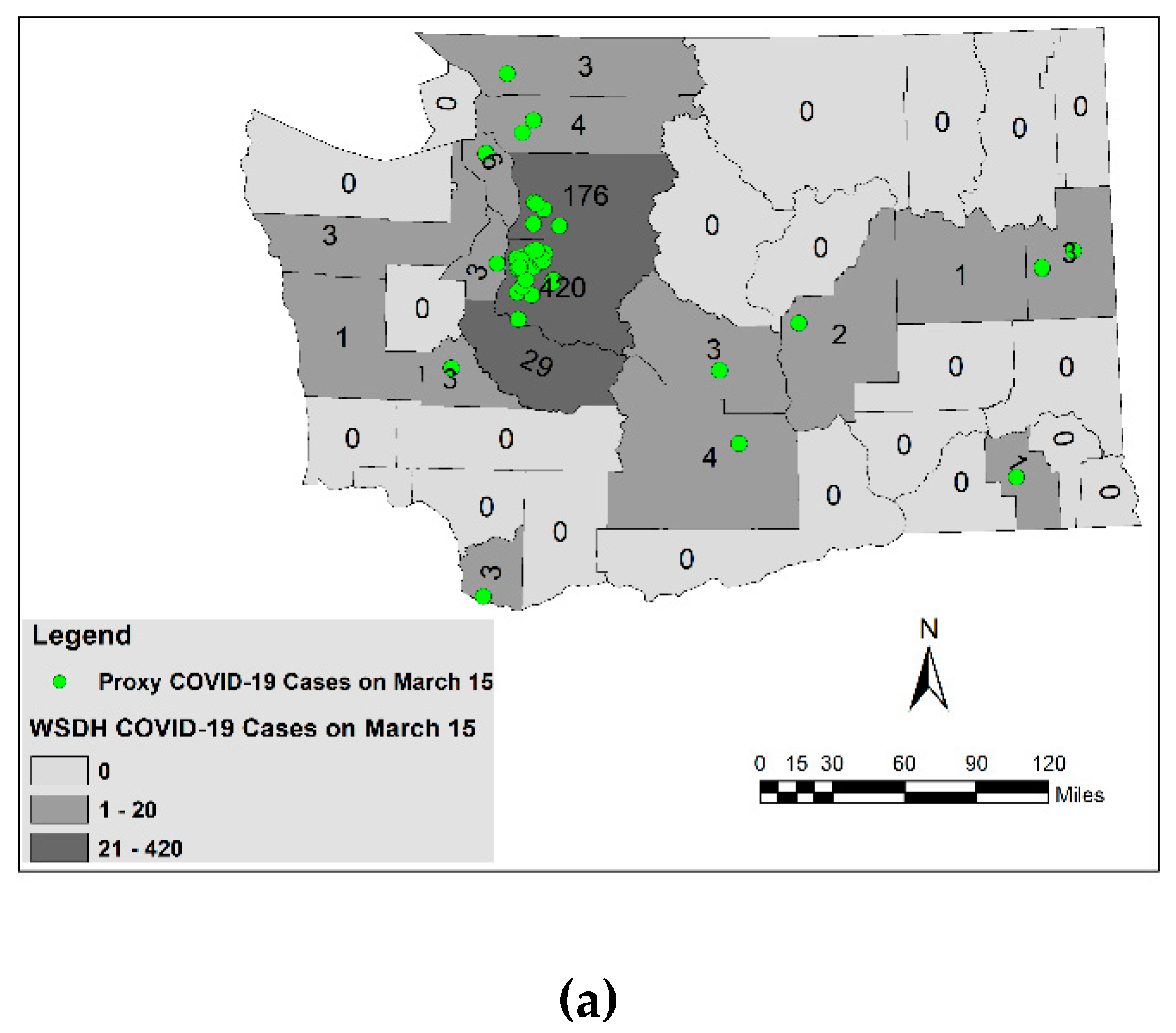
Note that the location information in this dataset is not the exact residential location of any of the patients, and hence, the author refers to these locations as proxy locations. For example, if the news reported that “a Fred Meyer employee who works at the Monroe location at 18,805 State Route 2 tested positive for coronavirus”, the Monroe location “Fred Meyer grocery store located at 18,805 State Route 2”, i.e., the work location of the patient, was marked as a proxy location for the patient. Similarly, if the news reported, “Officials say the Snohomish County case involves a Jackson High School student who is currently in home isolation”, the location of the school was marked as the proxy location. If a hospital was reported as “hospitalized at Valley Medical Center in Renton”, the hospital location was utilized. In cases in which only county names were revealed, for example, Douglas, Whitman, Adams, and Clallam County cases, the context was used to mark the proxy locations either at the nearest town or the nearest hospital. Here, the assumption is that, on average, a patient lives within a 15-mile (approximately 24 km) radius from the work location, hospital, university, or school [22]. This distance could be less for universities, schools and people working at local grocery or food chain locations [23]. The goal of this research is not to pinpoint and identify the exact residential location of a patient, but to identify a proxy location such that it can help in gaining insights into the space–time spread of COVID-19 during the initial stage of the outbreak. Although proxy locations are identified at a very detailed level, they do not expose or invade any patient’s privacy by identifying the residential location or identity in any way, but they still provide a good estimate for COVID-19 spread. The author does not claim to have retrieved an exhaustive record of all COVID-19-infected cases during the timeframe mentioned above. Instead, the dates and locations of every first case appearing in a new county are considered to be a sufficient sample for this study to understand the timeframe of COVID-19 spread from one location to another. Figure 4 displays proxy COVID-19 locations overlaid on top of WSDH COVID-19 case counts per county. A visual analysis shows that proxy locations collected in this study confirm the locations of cases identified by WSDH on 15 March (see Figure 4a) and 23 March (see Figure 4b). The author considers proxy locations valid since there is a good chance that patients might have exposed other people to COVID-19 at these proxy locations or within a 15-mile radius of commute distance. All proxy locations were projected to “NAD_1983_HARN_StatePlane_Washington_North_FIPS_4601_Feet” in order to perform statistical analyses based on distance.

2.3. Mapping Spread of COVID-19 in Space and Time

Typically, for point location datasets, statistical point pattern analysis is used to understand whether an observed pattern in the dataset is a result of a particular process. However, in the case of this study, there is no doubt that infected cases are observed due to the presence of the infectious COVID-19 virus. With this observation, the focus of this research is not on understanding the process causing the pattern but on understanding the pattern and its spread in space and time.

In order to map and understand the distribution of COVID-19 in WA over space and time, graphical methods, along with spatial point pattern analysis, were used. The goal is to map and analyze where COVID-19 proxy locations were concentrated and when and how they spread in time. Spatial statistical visualization and spatial measures of dispersion, such as kernel density estimation (KDE) and standard deviation ellipse (SDE) [24], were implemented to analyze spatial locations of COVID-19. Detailed descriptions of these methods are provided by Souris [24] and hence are not repeated here. These methods directly analyze spatial locations of COVID-19 and provide insights into its space–time spread. Moreover, attributes of COVID-19 cases were combined with these methods to gain geospatial insights into how COVID-19 spread from one location to another. Datasets were divided into four different time intervals, and KDE was implemented: (1) 21 January to 4 March (2) 5 March to 9 March, (3) 10 March to 15 March, and (4) 16 March to 23 March. Similarly, SDEs were calculated for three different time intervals: (1) 21 January to 6 March, (2) 21 January to 15 March, and (3) 21 January to 23 March. These time intervals were carefully selected so as to reflect the spread of COVID-19 into different parts of WA with time.

3. Results

The goal of this research is to gain insights into the spread of COVID-19 from patient zero’s location to other locations in WA with the progression of time. Given the infectious nature of COVID-19, it can be expected that during the initial stage of the outbreak, infections spread within neighborhoods close to patient zero. These close neighborhoods refer to areas that are frequented by people, for example, locations such as workplaces, grocery stores, shopping malls, schools and colleges, social gatherings, and public transit. Unless a new case of international exposure to COVID-19 is introduced in an area, infections will spread only from existing cases. New cases of COVID-19 will diffuse from the center of the outbreak to outer counties, exhibiting a clear space–time pattern unless interrupted by people traveling from other counties to infected locations and vice versa.

3.1. Spatial Analysis of Initial Spread

Two of the initial cases in the dataset are known to have traveled to Wuhan, China, and South Korea, countries with known cases of COVID-19 in January 2020. Visual analysis of two cases with a history of international travel (see Figure 5) reveals that the first case, i.e., patient zero, was identified in Snohomish County, in the extreme north of the map (red point), while the second case is known to have traveled far south on the map, near the border of King and Pierce Counties. This second case is referred to here as patient one. Patient zero and patient one tested positive on 21 January 2020, and 25 February 2020, respectively. Interestingly, almost all cases during the initial phase of the outbreak—from 21 January to 6 March 2020 (see Figure 5)—were located in close proximity and among known positive cases who had traveled internationally. This highlights the wide infection spread within the community in these two counties in the given timeframe. As discussed in the study area section, King County is a prime location for businesses. It is common for people from both King and Snohomish Counties to use public transit to travel between home and work locations.

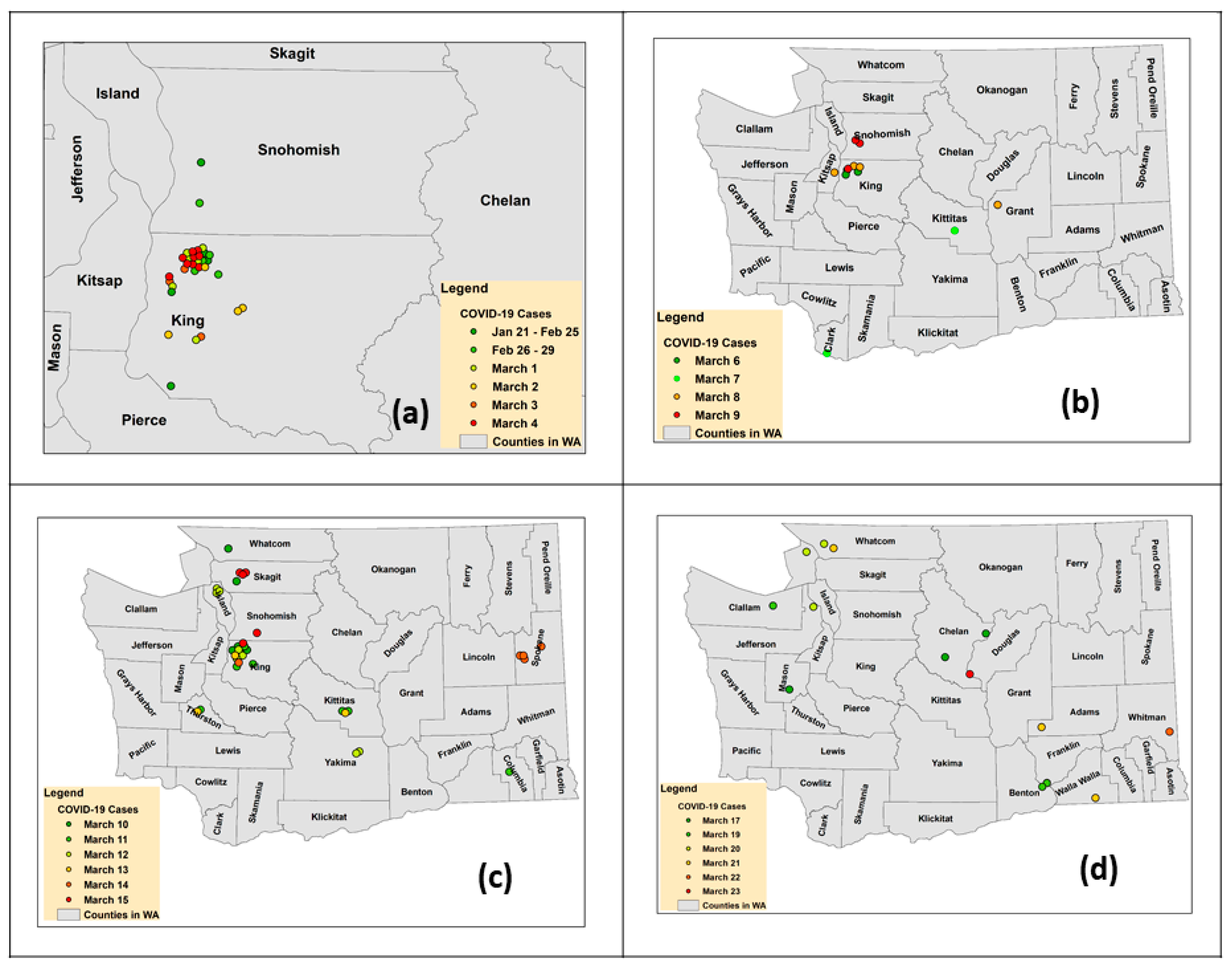
Figure 6 depicts proxy locations of COVID-19 cases in WA over time. Note that ArcGIS Pro’s disperse markers tool was used to create a representation such that overlapping or close proximity COVID-19 cases are spread apart for the purpose of clear visualization. A visual analysis shows clusters of COVID-19 cases in space and time: green points are clustered together from 21 January to 29 February (see Figure 6a). Orange-red points are clustered together from 2 March to 4 March. It can be expected that these clusters would appear to be more prominent in authentic COVID-19 location datasets. It would be valuable to study whether patient zero and its related cases of community infection could have been a primary source of spread until at least 11 February to 24 February, after which patient one might have contributed to the spread from another location. Here, the assumption is that patient one may have contracted the infection anywhere between 1 and 14 days prior to testing positive [4].

On 28 February, a new case was identified within 15 miles (24.1 km) of patient zero. This new case was a student from Jackson High School (JHS) in Everett and had shown symptoms on 24 February [25]. Figure 7 shows proxy locations of patient zero, patient one, the JHS-related case, and all other infected case proxy locations identified in this study. Typically, symptoms of COVID-19 appear anywhere between 2 and 14 days after exposure [4]. Given the gap of approximately 5 weeks between the 20 January date for patient zero and 28 February for the JHS case, it is difficult to conclude that the JHS case contracted the infection directly from patient zero, even though these two cases are located within close proximity. It is possible that a chain of community spread had been prevailing. This assumption is supported by an interesting study conducted on genomic epidemiology [26]. Dr. Bedford found that the COVID-19 virus exhibits minor mutations, twice a month, on average, while accumulating changes and remaining genetically identical during transmission from one person to another. This makes it possible to track the spread of the virus as it transmits from one person to another during an average of 7 days. This means that as the virus transmits from person 1 to 2 and from 2 to 3, the first mutation could be noticed. As it transmits from person 3 to 4 and 4 to 5, a second mutation is possible. On average, with two mutations, there will be five infected cases within one month or less. A similar process was observed in the case of patient zero and the JHS case, in that the JHS COVID-19 case was genetically identical to that of patient zero, with three mutations in the virus [26]. This suggests the presence of community-wide spread in the area. Even though the JHS case did not directly contract the infection from patient zero, patient zero might have transmitted it to other people who formed a chain before reaching the JHS case [26]. The fact that other cases were identified in King and Snohomish Counties from 19-26 February supports this notion. Such analysis with authentic data can reveal crucial insights into the distance at which diffusion occurs from the source location to other locations. If such distances are identified using authentic datasets, it can help in understanding and modeling the diffusion at finer scales.

3.2. Kernel Density Estimation (KDE) of COVID-19 Cases

One of the goals of this research is to understand the spatial extent to which the pattern of COVID-19 cases changed between 21 January and 23 March. Given the infectious nature of COVID-19, it is anticipated that cases have diffused over large distances in space with time. COVID-19 proxy point location data themselves do not provide information about change over time, nor do they provide insights into how it spread. In order to visualize the spread of COVID-19 from 21 January to 23 March, KDE was computed for different time intervals to convert proxy location points into density surfaces (see Figure 8).

The spatial distribution of cases from 21 January to 4 March (see Figure 8a) reflects the concentration of initial cases in the west-central portion of WA. Cases were prevalent only in King and Snohomish Counties, in close proximity of patient zero and patient one. From 5 March to 9 March (see Figure 8b), as more cases continued to appear in King and Snohomish Counties, the first cases appeared in new counties, such as Kittitas, Grant, and Clark. Exposure of patients to COVID-19 in new counties remains unreported or unknown. However, it is possible that these cases might have come in contact with cases from previously infected counties. From 10 March to 15 March, four distinct clusters can be observed in the west-center, center, east-center, and southeast (see Figure 8c). Cases of COVID-19 from the original cluster in King and Snohomish Counties had diffused to neighboring counties in the northwest, such as Skagit, Whatcom and Island Counties, and Thurston County in the southwest. In the central cluster, out of three new cases identified in Kittitas County from 11 March to 13 March, one case had known exposure to an infected case, while the second case was a relative of a previously infected person in the county. Two cases identified in Yakima County, a neighbor of Kittitas County, had known exposure to a woman from Kittitas County, thus forming a second cluster on the map and providing insights into community spread in spatially closer locations. The third cluster was seen on 11 March in Columbia County, which is not an immediate neighbor of any of the infected counties, but rather far away. This is explained by the known international travel associated with this new case. The fourth cluster was observed in Spokane County, with four new cases. Although there has been no report of how the first case was infected, it is known that all other three cases had attended a school event at which they came in contact with the first case. Between 17–23 March (see Figure 8d), three new dominant clusters appeared in farther counties in the northwest, southeast, and central WA. COVID-19 had diffused further to new counties, such as Mason, Clallam, Jefferson, and San Juan in the northwest; Franklin, Bento, Walla Walla, Adams, and Whitman Counties in the southeast; and Chelan and Douglas Counties in the center. Note that Figure 8d shows only new cases that were detected from 17–23 March. This does not indicate a decline in the number of cases in existing counties. In fact, cases continued to grow in these counties, but unfortunately, given the high number of cases in existing counties, details of new cases were not reported by news agencies. In the southeast cluster, a new case with a history of international travel appeared in Franklin County on 17 March. Following this, new cases were detected in the same county and in neighboring counties, such as Benton on 19 March and Walla Walla County on 21 March. However, exposure in these cases was not reported. In the northwest cluster, new cases that appeared in Clallam County on 19 March had known exposure to a King County connection, while the Jefferson County case detected on 20 March had traveled within the country. As the number of cases increased with time, there were fewer details in the information provided about each case; only county names with few details were revealed. These cases are still of importance for this study, as they appeared closer to infected counties rather than in completely isolated locations. Although the presence of community spread cannot be confirmed with this information, it can neither be denied. Further analysis with real-world data can reveal exact spread patterns. Nevertheless, the current analysis shows clear signs of community spread, but, more importantly, these clusters evolved over time while appearing in new and distant locations. This analysis clearly displays the diffusion of COVID-19 cases from King and Snohomish Counties located in the center of WA towards distant counties with the progression of time. From 21 January to 6 March, which is a duration of more than a month, known non-travel-related COVID-19 cases continued to appear only in King and Snohomish Counties. Diffusion to other neighboring counties was observed only after 6 March. This suggests that enough time was available during the initial stage to implement preventive control strategies. Appropriate social distancing strategies, if implemented during the very initial stage of such infectious diseases, could help in suppressing the diffusion over farther distances and to new locations with time. As described by Hua and Shaw [11], “having correct and timely information is crucial for stopping its spread, as well as in the curative prevention of this disease.”

3.3. Spatial Distribution of COVID-19 over Time

In order to understand the directional trends of the spatial distribution of COVID-19 cases over time, SDEs were calculated for three different time intervals (see Figure 9). SDE from 21 January to 6 March shows that COVID-19 cases followed a narrow north–south trend. Spread was more rapid in the Y-direction than in the X-direction, and cases were seen dispersed from Snohomish County in the north to neighboring King County in the south. The fact that this narrow spread was concentrated specifically towards the western edges of both the counties seems unsurprising because of the presence of a high population density, as well as the presence of patient zero in Snohomish County. As described in Section 2.1, both these counties are prime locations for major companies with strong public transit set-ups, and it is common for people to commute daily between these counties. A major highway, I5, connects these counties for daily commutes between residential areas and technology companies.

From 21 January to 15 March, the trend appears to have been spread slightly more in the northwest–southeast direction that covers more area, with new cases appearing in existing counties as well as moving into new counties. The spread in the X-direction reflects how new cases appeared in neighboring counties towards the northwest of Snohomish County and southeast of King County. According to the SDE for 21 January to 23 March, the trend changed direction more towards the northwest and southeast, continuing to spread rapidly in the X-direction. Cases with no international travel-related history appeared, especially in new counties in the north, northwest, center, and southeast.

Although the spread of cases was rapid from 21 January to 5 March, all new cases were observed strictly within Snohomish and King Counties (see Figure 6b). Between 6–9 March, cases spread to Kittitas and Grant Counties in the center and Clark County towards the southwest (see Figure 6b). From 10–15 March, cases appeared in communities that neighbor infected counties. For example, counties such as Skagit, Whatcom, and Island, located farther in the northwest and closer to King and Snohomish Counties, and Yakima County, located in the center and neighboring Kittitas (see Figure 6c). Infections in Spokane County towards the east were detected on 14 March. Finally, by 17–23 March, the farthest counties in the northwest and southeast had discovered their first cases of COVID-19, for example, new counties such as San Juan, Clallam, and Jefferson in the northwest and Benton, Walla Walla, and Whitman in the southeast. Although cases with histories of international travel appeared in Columbia and Franklin Counties in the southeast on 11 March and 17 March, respectively, cases without any history of travel were observed in this area only after 19 March. However, it is not clear if other cases are the result of diffusion from the new case with a history of international travel or if they can be attributed to the diffusion of infections from close contact in other infected counties.

This analysis shows clear directional trends and diffusion in space and time. The most important takeaway from this analysis is that it takes at least a few days for the diffusion of COVID-19 infections from existing cases during the initial stage of the outbreak. This can be a crucial window during which immediate preventive social distancing measures can help curb the diffusion. For such infectious diseases, time is extremely important during the initial stage. This is because, during the initial stage of the outbreak, the spread of COVID-19 seems to be confined within smaller areas. As time progresses, with no strict preventive social distancing measures, infections diffuse to new and distant locations, thus acting as new sources for infection. If not contained during the crucial window, infections tend to grow exponentially.

4. Discussion and Conclusions

This study has three primary objectives: (1) to create a proxy location and attribute data of COVID-19 cases in WA during the initial stage of the outbreak using publicly available news reports, (2) map the spread of COVID-19 in space and time and (3) use proxy datasets to gain insights into where, when, and how COVID-19 spread during the initial stage of the outbreak in WA. It is important to understand the extent of spread with time. This information could be useful for considering appropriate preventive and mitigation measures to possibly slow and reduce the spread in affected locations. Time, along with locations, plays an important role since it aids in understanding how fast infections spread to new and farther locations from the epicenter, i.e., patient zero.

In this study, the first objective was achieved by creating a proxy location and attribute datasets for COVID-19 cases in WA during the initial stage. The author acknowledges that these datasets are not complete, and some of the COVID-19 cases identified during the initial stage might not have been reported by news agencies and, therefore, not included in this study. Additionally, this study does not attempt to create an exhaustive list or accurate location information for all COVID-19 cases until March 23. The goal is rather to extract location, time, and attribute information for each new case identified in a new location. Such proxy data, though limited in terms of completeness, have still proven to be useful in providing insights into the spread of COVID-19 in space and time. The finest level of publicly accessible data for COVID-19 cases for the USA was available only as counts at county levels. Datasets aggregated as counts at the county level can be useful at best to create web dashboards. However, such datasets do not aid beyond geovisualization in order to perform spatial analysis for gaining further insights. Such data have very limited usefulness in terms of understanding the spread in space–time at a detailed level. The absence of attribute information further paralyzes the process completely, making it difficult to understand how infections have spread. Attributes obtained along with location information aid further in understanding not only where and when but also how COVID-19 cases diffused in WA. This study demonstrates that it is possible to create proxy datasets at a useful level, which could be used further for spatial analysis. Suggestions for further research include the automation of data extraction from unstructured text to replace the time-consuming manual process. For example, natural language processing techniques could be used to scan online news articles to extract place names and associated attribute data quickly.

The second and third objectives in this study were achieved by performing spatial analysis and creating KDS and directional trend analysis using SDE. Spatial analysis using centrography-based descriptive statistics is possible with point datasets at a finer spatial scale. Proxy datasets created in this study lend themselves to space–time analysis. A recent study using data for the 1854 cholera outbreak in London revealed the absence of a clear space–time pattern, supporting John Snow’s argument that cholera is a waterborne disease rather than an airborne one [27]. In WA, COVID-19 has spread continually since 21 January. Unlike Shiode’s cholera disease analysis [27], COVID-19 proxy data analyses show a clear space–time pattern, confirming that COVID-19 spread rapidly in neighboring communities during the initial stage of the outbreak. Strong community spread within Snohomish and King Counties is observed from 21 January to 6 March. It is only after 6 March that cases spread beyond the source, i.e., patient zero’s location. This provides useful insights into the timeline of spread to locations far from patient zero. More than a month, or about a 40- to 45-day window, passed before COVID-19 infections spread to new distant locations. However, it was not until 23 March that a clear stay-at-home order was announced by the governor of WA as a measure of social distancing [28]. Limits on large events were announced on 11 March, school closures were implemented on 13 March, and the shutdown of restaurants and limits on social gatherings were put in place on 16 March. The University of Washington transitioned to online instruction on 9 March [29]. This study suggests that identifying locations of infections and tracking their spread in space and time are crucial during the initial stage. Aggressive social distancing measures can help to slow and reduce the spread in space and time much more effectively if implemented in the initial stage. However, with a delay in implementing strict social distancing measures, new sources of COVID-19 infections are seen forming in new counties after 6 March. This continues to add to the rapid diffusion of infections to neighboring counties. Delaying aggressive social distancing will only worsen the situation and spread infections over farther distances. In fact, a recent study [11,13] presented a non-spatial analysis that demonstrated how aggressive social distancing measures have helped to curb COVID-19 spread in some countries. The current study provides spatial and temporal insights that suggest that although COVID-19 spread rapidly in WA, upon closer examination, infections were concentrated in specific areas of King and Snohomish Counties only. It took more than a month for infections to diffuse to other neighboring and distant locations. This implies that a broad window was indeed available for implementing preventive social distancing measures.

In this research, statistical analysis of point datasets is restricted to centrography-based descriptive statistics, such as kernel density estimation and standard deviation ellipse. Geovisualization of proxy point dataset provides a fair understanding of changes in the space–time pattern of locations and diffusion of infected cases. Although other intensity measures, e.g., spatial variation of points-based methods, can be implemented for analyzing point patterns, the current samples of proxy datasets do not lend themselves to such statistical tests. Even though results could be obtained by performing such analyses on the proxy datasets created in this research, they would not lead to accurate conclusions regarding the clustering of cases. Of course, it is observed that cases of infections appear to be clustered on the map, which cannot be denied. In fact, simple spatial analysis has shown that cases are located in areas that are highly populated and the most diverse. Given the infectious nature of COVID-19, clusters are expected in densely populated areas. However, identifying how clustered these infections are not the focus of this research. It would be worth studying such first-order effects and clustering using authentic datasets. Moreover, it would make more sense to study second-order nonstationary effects to understand whether cases are clustered in specific locations for a reason; for example, did people who use public transportation during a certain time period test positive, or did people in a certain community or demographic group who interacted either at work or socially get infected? The anisotropic spreading process of COVID-19 can also be analyzed; for example, do areas along a certain direction that has a strong public transportation system report more cases of infections? Such analyses are meaningful only when real-world datasets are analyzed.

Nonetheless, this research is still novel and important. It contributes to the current understanding by demonstrating the capability of generating proxy space–time data at a detailed spatial resolution from publicly available news articles. Such an approach for creating and analyzing preliminary proxy data is useful when real data are either totally absent or publicly available only at the county level. Analyses using proxy data provide valuable insights into space–time changes in the spread of COVID-19 within a single county and from one county to another. Using only publicly available county-level spatial data, it would not be possible to perform statistical procedures such as KDE and SDE to produce such space–time patterns to understand how infections spread over time at detailed spatial resolutions. Temporal data are extremely important in this research. This information provides insights into the time it took for the diffusion of infections between the date of the first reported case and the appearance of new cases within a county and in immediately neighboring counties. This crucial information tells us that, in the case of WA, starting from the initial stage when the first case was confirmed, new infections spread only in neighboring locations. Unless a person from a faraway location came in close contact with an infected person or location, it took a couple of days for the situation to worsen and spread to outer areas or counties within the state. This time lag between diffusion indicates that implementing immediate social distancing practices in infected locations and preventing travel from and to infected locations can prevent such situations from turning into pandemics. It would be interesting to conduct similar space–time studies in other states and countries to understand how long it took COVID-19 to spread from the location of the first detected case to more distant locations, with or without outer influence from international travel. The author will continue to study the relationship between COVID-19 locations and other factors that contributed to the rapid spread in WA.

References

1. World Health Organization. Disease outbreaks. Available online: https://www.who.int/emergencies/diseases/en/ (accessed on 29 March 2020).
2. World Health Organization. Pneumonia of Unknown Cause–China. Available online: https://www.who.int/csr/don/05-january-2020-pneumonia-of-unkown-cause-china/en/ (accessed on 29 March 2020).
3. World Health Organization. Naming the Coronavirus Disease (COVID-19) and the Virus that Causes It. Available online: https://www.who.int/emergencies/diseases/novel-coronavirus-2019/technical-guidance/naming-the-coronavirus-disease-(covid-2019)-and-the-virus-that-causes-it (accessed on 29 March 2020).
4. Centers for Disease Control and Prevention. How Coronavirus Spreads_CDC. Available online: https://www.cdc.gov/coronavirus/2019-ncov/prevent-getting-sick/how-covid-spreads.html (accessed on 29 March 2020).
5. World Health Organization. WHO Director-General’s Opening Remarks at the Media Briefing on COVID-19–11 March 2020. Available online: https://www.who.int/dg/speeches/detail/who-director-general-s-opening-remarks-at-the-media-briefing-on-covid-19---11-march-2020 (accessed on 29 March 2020).
6. British Broadcasting Corporation, Coronavirus_ Worst-hit Countries Boost Containment Efforts. Available online: https://www.bbc.com/news/world-51625123 (accessed on 29 March 2020).
7. Centers for Disease Control and Prevention. First Travel-Related Case of 2019 Novel Coronavirus Detected in United States_CDC Online Newsroom_CDC. Available online: https://www.cdc.gov/media/releases/2020/p0121-novel-coronavirus-travel-case.html (accessed on 21 January 2020).
8. Centers for Disease Control and Prevention. Situation Summary_CDC. Available online: https://www.cdc.gov/coronavirus/2019-ncov/cases-updates/summary.html?CDC_AA_refVal=https%3A%2F%2Fwww.cdc.gov%2Fcoronavirus%2F2019-ncov%2Fsummary.html (accessed on 29 March 2020).
9. Washington State Department of Health. Novel Coronavirus Outbreak 2020 (COVID-19)_Washington State Department of Health. Available online: https://www.doh.wa.gov/Emergencies/Coronavirus (accessed on 25 March 2020).
10. The New York Times. Coronavirus Slowdown in Seattle Suggests Restrictions Are Working-the New York Times. Available online: https://www.nytimes.com/2020/03/29/us/seattle-washington-state-coronavirus-transmission-rate.html (accessed on 29 March 2020).
11. Hua, J.; Rajib, S. Corona Virus (COVID-19) “Infodemic”and Emerging Issues through a Data Lens: The Case of China. Int. J. Environ. Res. Public Health 2020, 17, 2309. [Google Scholar] [CrossRef] [PubMed] [Green Version]
12. Johns Hopkins University. Coronavirus COVID-19 (2019-nCoV). Available online: https://gisanddata.maps.arcgis.com/apps/opsdashboard/index.html#/bda7594740fd40299423467b48e9ecf6 (accessed on 29 March 2020).
13. Dong, E.; Du, H.; Gardner, L. An interactive web-based dashboard to track COVID-19 in real time. Lancet Infect. Dis. 2020, 20, 533–534. [Google Scholar] [CrossRef]
14. World Health Organization. Coronavirus Disease (COVID-19) Situation Dashboard. Available online: https://covid19.who.int/ (accessed on 29 March 2020).
15. Kamel Boulos, M.N.; Estella, M.G. Geographical Tracking and Mapping of Coronavirus Disease COVID-19/Severe Acute Respiratory Syndrome Coronavirus 2 (SARS-CoV-2) Epidemic and Associated Events Around the World: How 21st Century GIS Technologies are Supporting the Global Fight Against Outbreaks and Epidemics. Int. J. Health Geogr. 2020, 19, 1–12. [Google Scholar]
16. Centers for Disease Control and Prevention. Cases in U.S._CDC. Available online: https://www.cdc.gov/coronavirus/2019-ncov/cases-updates/cases-in-us.html#2019coronavirus-summary (accessed on 29 March 2020).
17. Holshue, M.L.; DeBolt, C.; Lindquist, S.; Lofy, K.H.; Wiesman, J.; Bruce, H.; Spitters, C.; Ericson, K.; Wilkerson, S.; Tural, A.; et al. First Case of 2019 Novel Coronavirus in the United States. N. Engl. J. Med. 2020, 382, 929–936. [Google Scholar] [CrossRef] [PubMed]
18. The New York Times. Coronavirus Cost to Businesses and Workers_ ‘It Has All Gone to Hell’. Available online: https://www.nytimes.com/2020/03/15/business/economy/coronavirus-economy-impact.html (accessed on 29 March 2020).
19. Shekhar, S.; Shekhar, A.H.; The MIT Press Reader. As COVID 19 Accelerates, Governments Must Harness Mobile Data to Stop Spread. Available online: https://thereader.mitpress.mit.edu/contact-tracing-covid-19/ (accessed on 29 March 2020).
20. Lyseen, A.K.; Nohr, C.; Sorensen, E.M.; Gudes, O.; Geraghty, E.M.; Shaw, N.T.; Bivona-Tellez, C.; IMIA Health GIS Working Group. A Review and Framework for Categorizing Current Research and Development in Health Related Geographical Information Systems (GIS) Studies. Yearb. Med. Inform. 2014, 23, 110–124. [Google Scholar]
21. Xun, S.; Kwan, M.-P. Introduction: Geospatial Health Research and GIS. Ann. Gis Geospat. Health Res. 2015, 21, 93–95. [Google Scholar] [CrossRef]
22. Kneebone, E.; Holmes, N. The Growing Distance between People and Jobs in Metropolitan America. Available online: https://www.brookings.edu/research/the-growing-distance-between-people-and-jobs-in-metropolitan-america/ (accessed on 20 November 2019).
23. Easton, S.; Ferrari, E. Children’s Travel to School—the Interaction of Individual, Neighborhood and School Factors. Transp. Policy 2015, 44, 9–18. [Google Scholar] [CrossRef] [Green Version]
24. Souris, M. Epidemiology and Geography: Principles, Methods and Tools of Spatial Analysis; John Wiley & Sons, Inc.: Hoboken, NJ, USA, 2019. [Google Scholar]
25. Associated Press and Herald Staff. Jackson High Student, Infected with Coronavirus, ‘Doing Well’. Available online: https://www.heraldnet.com/news/jackson-high-student-infected-with-coronavirus-doing-well/ (accessed on 29 March 2020).
26. Trevor Bedford. Cryptic Transmission of Novel Coronavirus Revealed by Genomic Epidemiology. 2020. Available online: https://bedford.io/blog/ncov-cryptic-transmission/ (accessed on 29 March 2020).
27. Shiode, N.; Shiode, S.; Rod-Thatcher, E.; Rana, S.; Vinten-Johansen, P. The Mortality Rates and the Space-Time Patterns of John Snow’s Cholera Epidemic Map. Int. J. Health Geogr. 2015, 14. [Google Scholar] [CrossRef] [PubMed] [Green Version]
28. Medium, and Governor Jay Inslee. Inslee Announces “Stay Home, Stay Healthy” Order. Available online: https://medium.com/@GovInslee (accessed on 23 March 2020).
29. University of Washington. Moving Classes Online and Concluding the Winter Quarter. Available online: https://www.washington.edu/coronavirus/2020/03/06/moving-classes-online-and-concluding-the-winter-quarter/ (accessed on 29 March 2020).
Figure 1. Status of worldwide confirmed cases of COVID-19 as of 26 March 2020 (Source: Johns Hopkins University [12,13]).
Ijgi 09 00382 g001
Figure 2. Washington State Department of Health (WSDH) announcement on 25 March 2020. (Source: WSDH).
Ijgi 09 00382 g002
Figure 3. Study area displaying counties and divided highways in Washington State overlaid on top of a satellite imagery base map.
Ijgi 09 00382 g003
Figure 4. Proxy COVID-19 locations overlaid on top of WSDH COVID-19 case counts per county: (a) 15 March 2020; (b) 23 March 2020.
Ijgi 09 00382 g004aIjgi 09 00382 g004b
Figure 5. Proxy locations of COVID-19 cases in Snohomish and King Counties in WA from 21 January to 6 March 2020.
Ijgi 09 00382 g005
Figure 6. Proxy locations of all COVID-19 cases in WA: (a) 21 January to 4 March; (b) 6 March to 9 March (c) 10 March to 15 March; (d) 17 March to 23 March.
Ijgi 09 00382 g006
Figure 7. Proxy locations of two patients infected during international travel and their proximity to all COVID-19 proxy locations from 19 January 2020 to 23 March 2020.
Ijgi 09 00382 g007
Figure 8. Kernel density estimation for COVID -19 spread during four time intervals: (a) 21 January to 4 March (b) 6 March to 9 March; (c) 10 March to15 March; (d) 17 March to 23 March.
Ijgi 09 00382 g008aIjgi 09 00382 g008b
Figure 9. Spatial distribution of COVID-19 cases and the corresponding standard deviation ellipses (SDE) from 21 January to 6 March (green), 21 January to 15 March (yellow), and 21 January to 23 March (red).
Ijgi 09 00382 g009