Abstract
The proliferation of high-resolution remote sensing sensors and platforms imposes the need for effective analyses and automated processing of high volumes of aerial imagery. The recent advance of artificial intelligence (AI) in the form of deep learning (DL) and convolutional neural networks (CNN) showed remarkable results in several image-related tasks, and naturally, gain the focus of the remote sensing community. In this paper, we focus on specifying the processing pipeline that relies on existing state-of-the-art DL segmentation models to automate building footprint extraction. The proposed pipeline is organized in three stages: image preparation, model implementation and training, and predictions fusion. For the first and third stages, we introduced several techniques that leverage remote sensing imagery specifics, while for the selection of the segmentation model, we relied on empirical examination. In the paper, we presented and discussed several experiments that we conducted on Inria Aerial Image Labeling Dataset. Our findings confirmed that automatic processing of remote sensing imagery using DL semantic segmentation is both possible and can provide applicable results. The proposed pipeline can be potentially transferred to any other remote sensing imagery segmentation task if the corresponding dataset is available.
1. Introduction
The rapid development of aerospace technology, that resulted in the availability of a large amount of satellites and aircraft platforms (both manned and unmanned), led to a much easier acquisition of high-resolution remote sensing imagery [1]. Unmanned airborne systems (UAS), particularly the class of UAS referred to as small-unmanned airborne systems (S-UAS), will not only enable a range of novel remote sensing capabilities but also present clear challenges to the remote sensing community including increased data volume and a paucity of appropriate analysis approaches [2]. With no shortage of data, the real challenge shifts towards the automated extraction of valuable information from them.
Remote sensing images are used for extracting and mapping objects such as buildings [3], roads [4], vehicles [5], ships [6], terrain features [7], etc. Pixel-wise labeling of remote sensing imagery corresponds to a semantic segmentation task defined in computer vision (CV). Automated semantic segmentation and annotation of objects found in urban areas play an important role in many remote sensing applications, such as building and updating a geographical database, land cover change, and extracting thematic information [8]. Building extraction is usually the most critical task since it is used to monitor changes in urban areas, urban planning, and estimating the population [1]. However, buildings are rich in diversity of visual features that make them much harder to identify compared to natural objects such as water bodies and forests, or even artificial objects such as roads and vehicles.
The recent advance of artificial intelligence (AI) in the form of deep learning showed remarkable results in several image-related tasks, and naturally, gain the focus of the remote sensing community. Deep learning is characterized by the use of neural networks usually involving many layers, so they are called ‘deep’. The introduction of a special kind of neural network called convolutional neural network (CNN) [9] revolutionized computer vision and made a huge impact on solving problems of image classification, localization, and semantic segmentation. Deep CNNs, through the many layers they have, are capable of building a hierarchy of features that makes them especially suitable for these tasks [10]. The ability to learn different data representations (i.e., features) makes deep CNNs extremely powerful in representing complex real-world images so they can be easily classified. This property of deep CNNs is especially important when dealing with building footprint extraction due to their visual diversity. The importance of classification CNN architectures lies in the fact that they can be relatively easily extended and used for semantic segmentation. There are many different architectures that arise in the past couple of years to tackle this problem. We will review them in the next section.
In this paper, we proposed an approach for automated processing of remote sensing imagery for the purpose of building footprint extraction using deep semantic segmentation. The method that we proposed represents a generic pipeline that consists of the three stages: image preparation, deep segmentation model implementation and training, and predictions fusion. For evaluation, we used Inria Aerial Image Labeling Dataset [11], which will be described in Section 3. Since the dataset authors organized a public competition, the official contest results are also presented and discussed in this paper.
The paper is organized as follows: Section 2 presents an overview of related work concerning deep semantic segmentation architectures and their use in remote sensing. Section 3 contains details regarding the used dataset. In Section 4, the proposed method is described presenting the processing pipeline. The results obtained from conducted experiments are presented and discussed in Section 5. Finally, Section 6 presents the conclusions.
2. Related Work
The use of deep CNNs represents the current state-of-the-art for image classification, object localization, and semantic segmentation in general. This approach has become exceedingly popular in the domain of remote sensing where the aim is to automate the processing of huge amounts of available aerial imagery. One of the earliest successful application of deep CNNs has been land-use classification [12,13,14]. As the name suggests, this task belongs to the image classification problem, where the idea is to train a deep CNN network to detect the category of land-use based on a small aerial image patch. To produce a land-use map for some area require using sliding window technique [15], i.e., to extracting successive patches (possibly with overlapping) and determine appropriate land-use class. This approach comes with two drawbacks: it is slow, and it tends to significantly reduce the resolution of the output map. An alternative approach would not be to classify the image patch as a whole, but to determine the class for each pixel in it. This pixel-level classification is known as semantic segmentation, and when it is done using deep CNNs it is usually referred to as deep semantic segmentation.
Deep CNN for classification can be seen as a generic feature extractor with a classifier on top of it, that is trained in an end-to-end manner. Layers in CNN tend to reduce the spatial dimension of the input and widen the feature dimension. If we chop off the classification part of the CNN, also known as the head, and attach different ‘head’ that upscales the last feature map (spatial dimension) and then reduce the number of channels (feature dimension) using additional convolutional layer, we end up with CNN for semantic segmentation known as Fully Convolutional Network (FCN) [16]. The described FCN architecture suffers from the fact that the spatial component of the last CNN feature map is several times smaller than the input size, so upscaling it does not bring the details back. To achieve better segmentation results it is possible to form a hypercolumn [17] using feature maps obtained from several stages of CNN. The number of filters in each feature map is equalized with additional convolutional layers and, after upsampling to a certain size, an additional operation is used to construct a hypercolumn that is used for pixel-level classification. DeepLab [18] architecture represents another direction for addressing the FCN issue of low-resolution predictions based on atrous convolutions.
More complex CNN architectures for semantic segmentation are DeconvNet [19] and U-Net [20]. Both networks share a similar architectural idea: the network consists of encoder and decoder parts. In the case of DeconvNet, they are called convolution and deconvolution networks, respectively. The encoder part is basically a classification CNN with a removed top, while the decoder has a mirrored structure with blocks that consist of upsampling or transpose convolution layers followed by convolutional layers. U-Net architecture, in addition, introduces skip connections that enable copying and concatenating earlier encoder feature maps to corresponding upsampled decoder feature maps, so decoder convolution layers process them both. A very similar approach, with slight differences, is promoted by SegNet [21] architecture.
Feature Pyramid Network (FPN) [22], which performed best in our experiments, has a similar structure to U-Net, e.g., it also has the lateral connection between the encoder (bottom-up pyramid in FPN representation) and decoder (top-down pyramid). The main difference is that FPN introduces multiple prediction layers, i.e., one for each upsampling layer. Additionally, while U-Net only copies and appends the features from the encoder to the decoder, FPN first applies 1 × 1 convolution thus allowing to use of arbitrary architecture for the bottom-up pyramid, i.e., ‘backbone’.
Deep semantic segmentation has been the topic of many research studies in remote sensing. Building footprint extraction, due to the importance and availability of datasets, has been the subject of many recent papers [1,3,23,24,25,26,27,28]. The listed papers examine different architectures and propose some adjustments to better cope with the problem. The focus of this paper is on specifying the processing pipeline that allows us to use existing state-of-the-art deep semantic segmentation models for automated processing of remote sensing images. In the case of building footprint extraction, we demonstrated a methodology, based on empirical examination, for selecting the optimal model.
3. Dataset
For the study presented in this paper, we used Inria Aerial Image Labeling Dataset [11] (hereinafter referred to as the Inria dataset). The dataset addresses one of the most important problems in remote sensing: the automated pixel-wise labeling of aerial imagery. In particular, the Inria dataset consists of aerial orthorectified color imagery with a spatial resolution of 30 cm per pixel, with appropriate ground truth data for two semantic classes: building and not building. The images cover dissimilar urban settlements, ranging from densely populated areas to alpine towns. An interesting property of the Inria dataset is that the train and test subsets contain imagery of completely different cities that enables evaluation of how the proposed labeling method generalizes to any city. The dataset was the basis for a contest held to compare different approaches to this problem. The corresponding contest results, along with the download files, are available at the dataset web page [29].
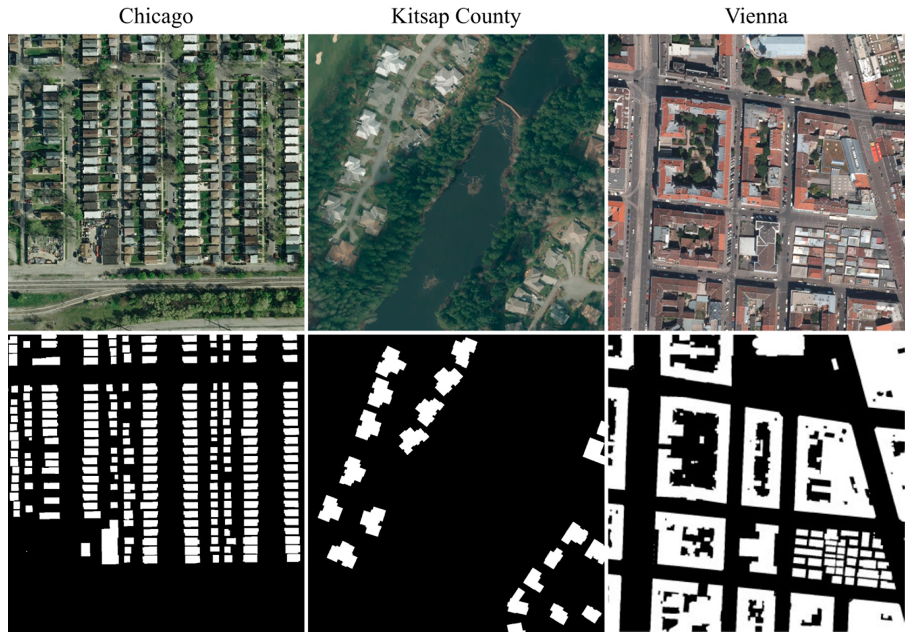
The Inria training set consists of 36 color image tiles of size 5000 × 5000 pixels for each of the following regions: Austin, Chicago, Kitsap County, Western Tyrol, and Vienna. That is a total of 180 images covering an area of 405 km2. Ground truth data consists of corresponding 180 single-channel images with value 255 for the building class and 0 for the not building class. The illustration of the Inria training dataset showing several image patches and corresponding ground truth is shown in Figure 1.

Figure 1.
Illustration of the Inria dataset showing three sample image patches and corresponding ground truth for Chicago, Kitsap County, and Vienna (source [29]).
For the competition purposes, the test set published contains the same number of image tiles, but this time for the following regions: Bellingham, Bloomington, Innsbruck, San Francisco, and Eastern Tyrol. Ground truth data for the test set is not disclosed. Model performance is measured using two distinct metrics: Intersection over Union (IoU) and accuracy. IoU is calculated as the number of pixels labeled as building in both predicted and ground truth images, divided by the number of pixels labeled as building in the predicted or ground truth image. Accuracy, on the other hand, represents the percentage of correctly classified pixels. These two metrics are computed for each of the five test regions separately and for the overall test set.
To calculate IoU metrics using ground truth (GT) and predicted mask (PM), as well as true positives (TP), false positives (FP), and false negatives (FN), we use the following equation:
Similarly, accuracy metrics can be calculated using TP, FP, FN, and false positives (FP) using the following equation:
Since the competition does not specify single metrics to evaluate results, we introduced ‘combined’ metrics to be able to select the best performing model during training. The combined metrics is calculated as the mean of IoU and accuracy:
Both IoU and accuracy metrics are equally weighted in the combined metrics, but IoU has a much stronger influence on the resulting metrics. The reason for that is the TN term found in the accuracy Equation (2) that is dominant and thus plateaus the metrics. This property of the combined metrics can be treated as the desired one since IoU is usually used for segmentation tasks.
4. Method Description
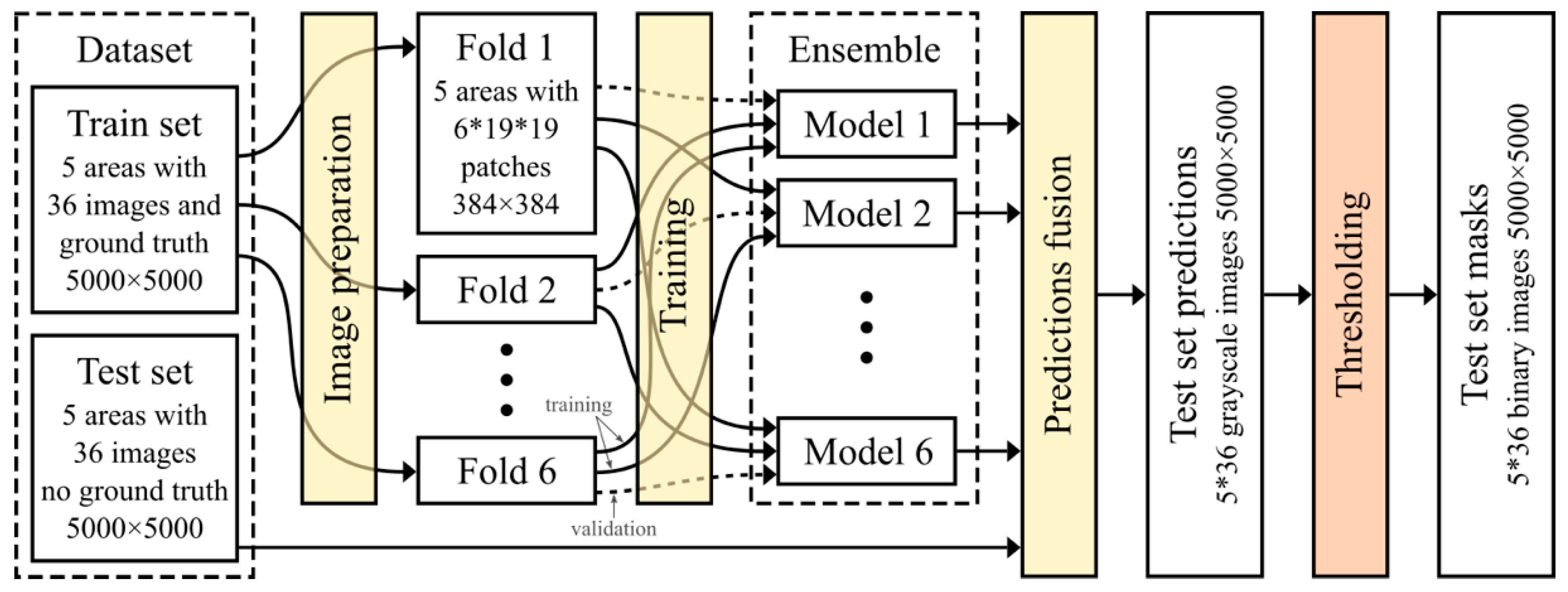
The method applied for processing of the Inria dataset involves image preparation, implementation and training of an ensemble of deep CNNs for semantic segmentation, and, finally, applying them to predict building masks for the test set image tiles (see Figure 2). Data split into 6 folds, which are used to train an ensemble of 6 models, was chosen, as each region has 36 images, so each fold used 6 of them for validation () and the remaining 30 for training (). The used data split into folds follows a suggestion by the dataset authors to use the first 5 images for each region for validation. A viable alternative to test would be to use 5 folds, one for each region, and train an ensemble of 5 models.
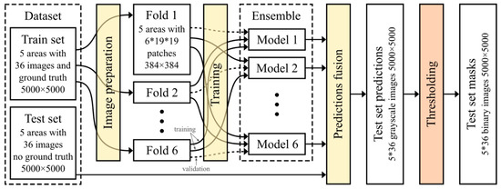
Figure 2.
Illustration of the proposed processing pipeline applied to the Inria dataset.
The following subsections explain how each of these subtasks is performed. It should be emphasized that the proposed pipeline is generic, and it can be applied to any similar problem related to the processing of remote sensing imagery.
4.1. Image Preparation
The first step in the pipeline for processing remote sensing imagery using deep semantic segmentation is to prepare input and ground truth images in a format applicable for training the appropriate models. This is achieved by extracting a series of patches, of the specified size, from original input and ground truth images. There are several ways the extraction could be achieved, but general rules are to allow overlapping of patches so that different parts of the image can be found in different locations in patches.
Our method for patches extraction relied on regular grid cutting with overlapping. Parameters that are specified to prepare patches are target patch size and percentage of minimal overlapping between nearby patches. Once the input image is loaded, based on these two parameters, a number of patches’ columns and rows are calculated, and patches are extracted using even distribution. For example, for Inria images that are 5000 × 5000 pixels, if target patch size of 384 × 384 pixels is selected and minimal overlapping of 30%, a total of 361, i.e., 19 × 19, image patches and exactly the same number of ground truth patches are extracted. Since the Inria training set contains 180 input images, that translates to a total of 64,980 input patches and the same number of ground truth patches.
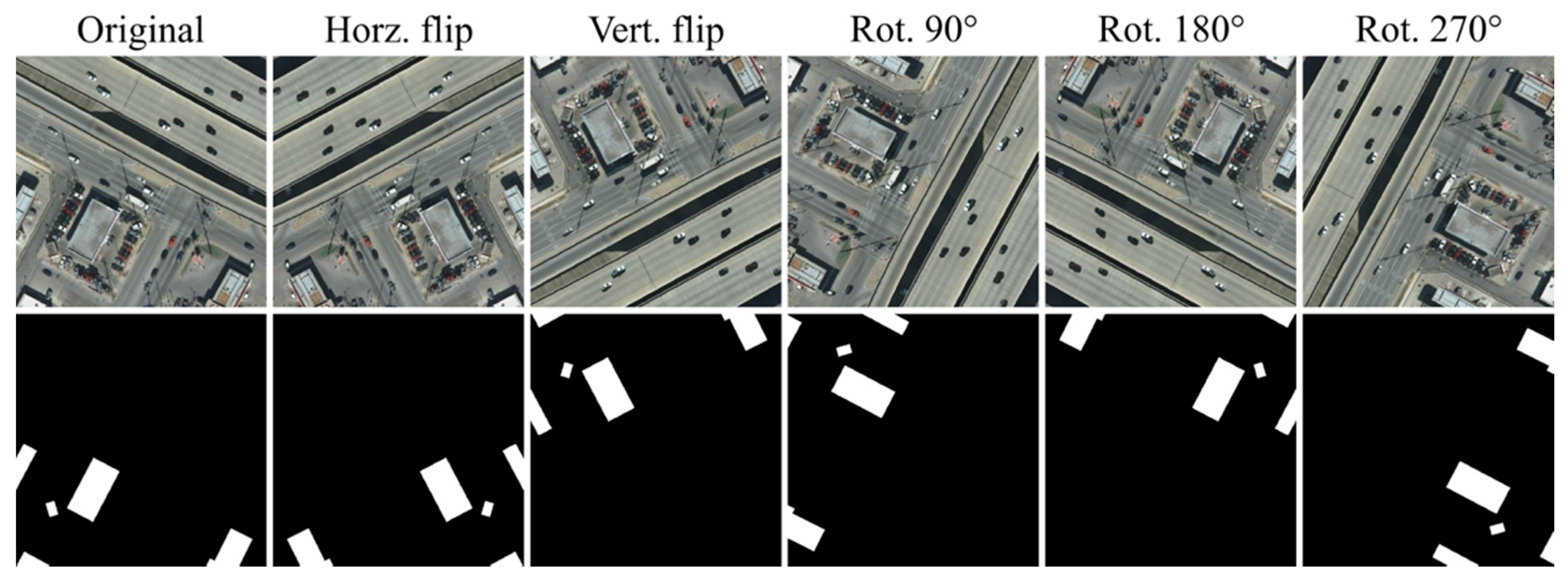
Besides overlapping, when processing aerial imagery, to further increase the diversity of the training dataset, a specific data augmentation technique is applied. This technique generates five variations of the original image by flipping the image horizontally and vertically, and rotating the image for 90°, 180°, and 270°. The illustration of the proposed data augmentation technique is shown in Figure 3. By applying this technique, an effective number of different patches used for training in the previous scenario is 6 × 64,980 = 389,880. Of course, to preserve the hard disk space needed for storing training patches, data augmentation is applied dynamically, by selecting and applying random transformation each time the patch is used for training.
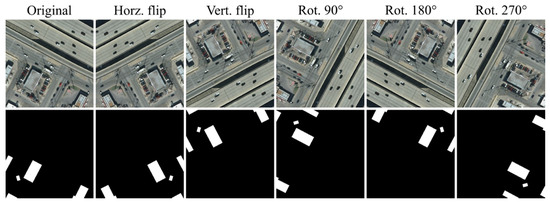
Figure 3.
Illustration of data augmentation technique that produces five variations of the original image and ground truth patches.
4.2. Predictions Fusion
In the previous subsection, we showed how to transform larger input images and ground truth masks to the format applicable for training deep semantic segmentation models. In this subsection, we are going to assume that we already have one or more trained models, and we will describe how they can be applied to obtain predictions and create output masks for the test images. The reason we are first jumping to the final step in the pipeline is due to the fact that it is, to some extent, the inverse of what we had in the image preparation step.
Since deep semantic segmentation models are trained using relatively small image patches, the predictions they are capable of producing are also relatively small. For that reason, again, we need to extract image patches from test images, use them to create appropriate predictions, and then somehow merge those partial predictions into a single output mask. In addition, it is possible that we trained not a single, but an ensemble of several models, so each of them can produce a different prediction for each input patch.
The term ‘prediction’ is used to depict a model output, that for the problem of binary segmentation, represent a matrix in which elements range between 0 and 1. Each element in the matrix corresponds to a pixel in the input image patch and can be interpreted as the probability that a certain pixel belongs to a building. If we deal with an ensemble of models, the integral prediction for an input patch is obtained by averaging predictions for each of the models in the ensemble.
The method of averaging can be further used to apply a technique called test-time augmentation (TTA). TTA is an application of data augmentation to the test data. In our case, it represents obtaining six predictions for each image patch and the five previously described transformations, then aligning them by applying appropriate inverse transformations, and again averaging them to produce a final prediction for the patch.
The third situation where prediction averaging is applied is when we merge separate patches’ predictions into an integral prediction for the whole image. The need for averaging comes from the fact that we applied the same patch extraction method as described in the previous subsection that involves overlapping. For this particular task, a weighted averaging is applied. The intuition behind it is that a deep semantic segmentation model, which is based on a CNN, will give better predictions in the central part of the image patch, due to more complete information, compared to the edges and corners. For that reason, when averaging predictions due to mergin, we decided to take the central part more into account than edges and, especially, corners. The way to do that is to multiply predictions with a 2-dimensional Gaussian kernel (see Figure 4).
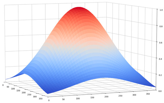
Figure 4.
The Gaussian kernel used for weighting segmentation model predictions.
Finally, the particular implementation of this step works as follows. For each input image, two zero-initialized matrices (prediction and impact) are created, dimensioned according to the input image size. For each extracted patch, TTA transformation, and model in the ensemble, a prediction is obtained. The obtained prediction is multiplied by the predefined Gaussian kernel and added to the prediction matrix, i.e., to the appropriate elements determined by the patch location. At the same time, the Gaussian kernel is added to the same elements of the impact matrix. After processing all patches, the final prediction for the input image is calculated by dividing the prediction matrix with the impact matrix. Figure 5 depicts an illustration of the weighted overlapping used to obtain integral predictions. To preserve detailed predictions, resulting elements are multiplied by 255, rounded and saved as a grayscale PNG image. The appropriate binary mask is created from the grayscale image by applying threshold operation at a certain level. The optimal threshold level is determined by evaluating IoU and accuracy metrics on the validation images and finding the maximum of the combined metrics, as shown in Figure 6.

Figure 5.
Illustration of the weighted overlapping used to obtain integral predictions.
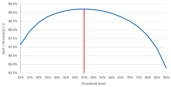
Figure 6.
Threshold level evaluation for converting grayscale predictions to binary masks.
4.3. Model Implementation and Training
The central part of the proposed method is the implementation and training of a deep semantic segmentation model capable of predicting where buildings are, given the input aerial image patch. The implementation was done using the Python programming language and Keras [30] library. Keras is a high-level library that defines a simplified interface for implementing deep neural networks, and in our case, it relies on TensorFlow [31] library as a backend engine. The source code for the project can be found at [32].
For the implementation of deep semantic segmentation models, we relied on Pavel Yakubovskiy’s Github library called Segmentation Models [33], a Keras-based Python library that implements four popular segmentation architectures and dozens of ImageNet pretrained backbones that can be easily combined into the segmentation model of choice. The library supports the following architectures: U-Net [20], FPN [22], LinkNet [34], and Pyramid Scene Parsing Network (PSPNet) [35]. To choose the architecture and backbone, we conducted a preliminary study where we trained and evaluated several available combinations, as depicted in Table 1. The depicted validation metrics are obtained directly from the training process of a single model for each combination of the segmentation architecture and backbone. We did not use evaluation based on predictions fusion at this stage because it had not been developed at that moment. This study was not exhaustive, especially when it comes to the available backbones (total of 24), and the reason for that is very long training time due to a large amount of data (training one model can take several days). For that reason, the idea was to test all four available architectures using relatively simple ResNet-34 [36] backbone and then run a couple more experiments with the winning architecture. In our study, FPN architecture performed best, so we ran two more experiments combining it with SEResNet-34 [37] and ResNeXt-50 [38] backbones. The reason for FPN performance can be found in its architectural property that involves multiple prediction layers, e.g., one for each upsampling layer. In our opinion, FPN’s multiple prediction layers play an important role in building footprint extraction due to the high diversity of sizes and types in which buildings are present, thus allowing the different prediction layers to detect different building types. In our experiments, we chose ResNet variations for the backbone for two reasons: the first is their relatively good performance on the ImageNet dataset, while the second is their ability to use a pretrained backbone with patches of various input sizes. The best results were achieved in combination with the ResNeXt-50 backbone, so for further experiments we stuck to that combination. A detailed illustration of the used segmentation model is depicted in Figure 7.

Table 1.
Results of the preliminary study applied to select the architecture and backbone.
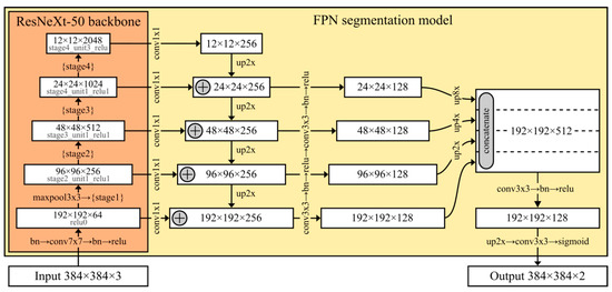
Figure 7.
A detailed illustration of the used segmentation model based on FPN and ResNeXt-50.
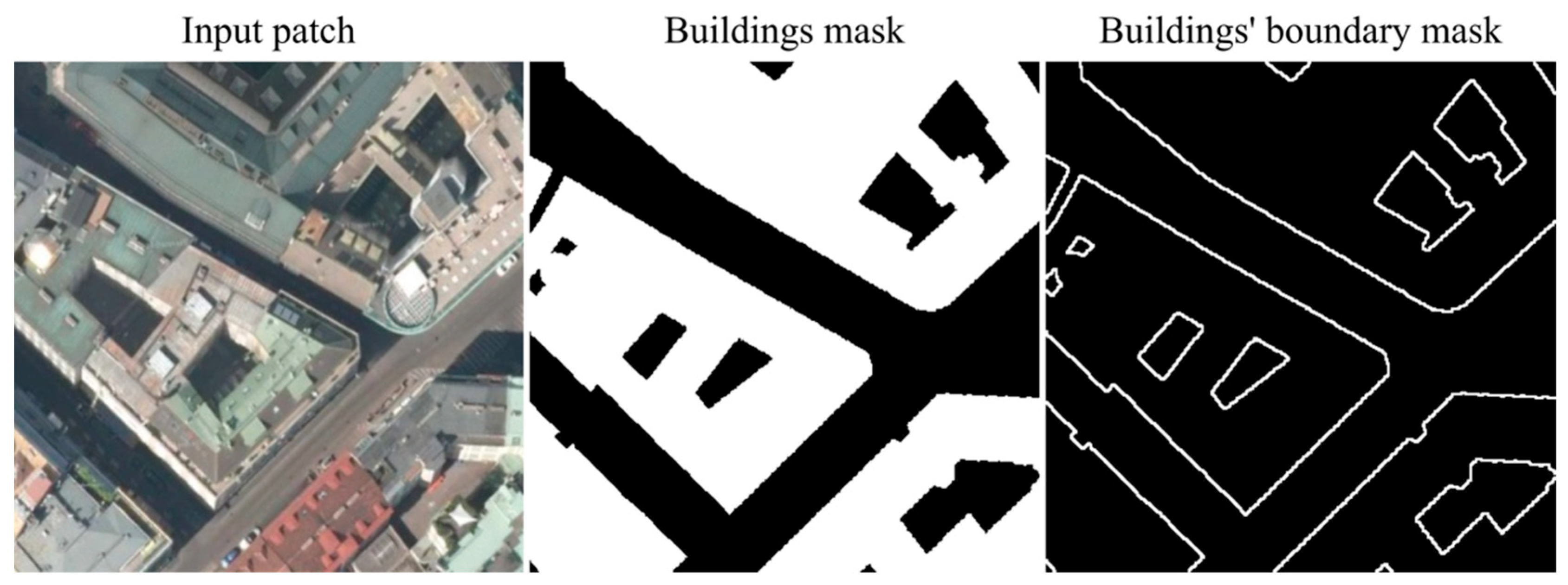
As can be seen in Figure 7, the segmentation model was trained using 384 × 384 patches. Input images have three channels for red, green, and blue color components, while the output prediction has two independent channels that are obtained using sigmoid activation. The first channel corresponds to a building/not building mask, and it represents an actual model output, while the second is only temporarily used during the training. The second channel corresponds to a buildings’ boundary mask, and it is introduced as a kind of ‘training helper’, so the model can learn features related to a boundary between buildings and their surroundings. This approach was introduced by Mou and Zhu [5] for the purpose of vehicle instance segmentation from aerial imagery. In our implementation, we stacked the original ground truth mask with a derived boundary mask that is produced by subtracting the eroded building mask from the dilated building mask (see Figure 8). The model is trained to learn both masks, but IoU and accuracy metrics are calculated only for the first channel. Similarly, when we need to apply such a model later, we simply discard the second channel and only use the first one as the prediction.
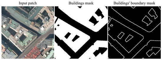
Figure 8.
An illustration of the derived buildings’ boundary mask channel that is used during the training of the segmentation model.
The training process was organized in two phases. In the first, i.e., the major training phase, the whole network was optimized using binary cross-entropy loss. After that, the network was fine-tuned in the second phase using the sum of binary cross-entropy loss and dice loss. Dice loss [39] corresponds to the IoU metric, so that is why it is introduced in combination with binary cross-entropy that corresponds to the accuracy metric. The term ‘fine’ is used to indicate that a smaller initial learning rate was used to preserve initial network parameters.
The created model was compiled using the ‘RMSprop’ [40] optimization algorithm (‘optimizers’ module), ‘binary_crossentropy’ loss (‘losses’ module), and three custom defined metric functions ‘acc_fc’, ‘iou_fc’, and ‘acc_iou_fc’. All three custom metrics extract the first output channel that corresponds to buildings mask and calculates ‘binary_accuracy’ (‘metrics’ module), batch level IoU (implemented in [33]), and mean of those two (combined metric), respectively. The optimization algorithm was chosen because of its fast convergence and relatively low memory footprint.
To support custom data augmentation and batch preparation, we the implemented ‘DataAugmentation’ class that inherits Keras’ ‘Sequence’ (‘utils’ module). The implemented class was also designed to support train and validation data split using 6 folds (see Figure 2). Since each region has 36 images, we use patches from 6 of them for validation and patches from the remaining 30 images for training. It is possible to select which fold is used for validation, so we were able to train a total of 6 different models that are used in the ensemble.
The training was initiated calling the model’s ‘fit_generator’ method. Additional control of the training process in Keras is possible using callback objects. The corresponding classes are located in the callbacks module and we applied the following ones: ‘LearningRateScheduler’, ‘EarlyStopping’, ‘ModelCheckpoint’, and ‘CSVLogger’.
‘LearningRateScheduler’ is used to specify an arbitrary function for calculating the learning rate depending on the current training epoch. We used this callback to implement the so-called cosine annealing [41]. In cosine annealing, the learning rate decreases following cosine function from some initial value to some minimum value during a certain number of epochs (period). In our implementation, with each new period, the initial learning rate was decreased by a factor of 0.7. We used the initial value of 10−4 for the first phase of the training and 10−5 for the fine-tuning. The minimum value was 0.01 times the initial value. The appropriate schedule, i.e., scaling of the initial learning rate, is shown in Figure 9.

Figure 9.
Cosine annealing schedule used for scaling the initial learning rate during the training.
‘EarlyStopping’ callback, as the name suggests, is used to stop the training process if there is no progress on a given parameter in some number of epochs. In our case, 10 epochs for initial training and 5 for fine-tuning were used and combined metrics (mean of accuracy and IoU) on the validation set was monitored. ‘CSVLogger’ callback is used to record loss and accuracy on the training and validation sets during the training process. Finally, ‘ModelCheckpoint’ was used to save the current best model in terms of accuracy achieved on the validation set.
The fine-tuning was done in an almost identical way, with a few minor modifications. After loading the model obtained from the first training phase, it was compiled, specifying a custom loss function ‘bce_dice_loss’, which is defined as the sum of previously used ‘binary_crossentropy’ (evaluated for both channels) and ‘dice_loss’ (implemented in [33]) that is evaluated on the first channel only. The second change affected the initial learning rate that was reduced to 10−5 to avoid significant weight changes in the network. The obtained results are presented in the next section.
5. Results and Discussion
For the evaluation of the proposed method, we trained and fine-tuned six models, changing the fold used for validation. The training was done on a single personal computer with an Intel i7-8700K processor, 32 GB of RAM, and a single Nvidia GeForce 1080 Ti with 11 GB of memory. Image patches of 384 × 384 pixels were used for both training and evaluation. The model has a total of 26,415,051 parameters, where 26,344,517 of them are trainable. Due to a significant memory footprint of the model, the batch size for the training was set to 8.
To train and fine-tune all six models it took more than three weeks. More precisely, the initial training phase took 19 days (~3 days per model), while the fine-tuning phase took 4.5 days (~1.5 days per model). As an illustration of the training process, in Figure 10 we depicted accuracy, IoU, and the combined metrics during the initial and fine-tuning training phases of the first model. The vertical red lines on the charts show the epochs where the biggest combined validation metrics are obtained, and the model is saved for later use.
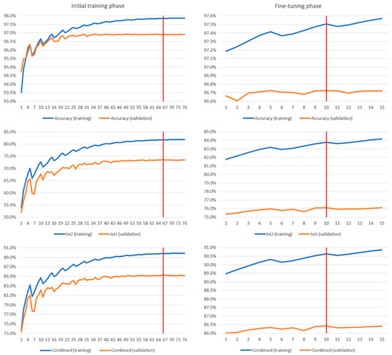
Figure 10.
Accuracy, IoU, and combined metrics charts during the initial and fine-tuning training phase of the first model.
Although the metrics obtained during the training process provide some information about expected model performance, to test it properly, along with the other proposed techniques for obtaining final predictions, the evaluation of each model is performed on the appropriate images that formed the validation set. In the case of the first trained model, validation images are 1 to 6 for each area of the training set. The time needed for the evaluation of a single trained model is 34 min. That involves creating predictions for 30 images of 5000 × 5000 pixels, so the average time for processing a single image is 68 s. Details for all five areas and all six images are shown in Table 2. The table also shows summary metrics for all six images per area and overall. Please notice that summary metrics are obtained for the image set as a whole, i.e., they are calculated tracking and summarizing the number of intersected, union, and total pixels in each of the images. This only affects IoU value, while the accuracy remains equal as if we averaged per image values.

Table 2.
Detailed evaluation results on the validation images (1–6) for the first model.
The summary evaluation results for all six models are shown in Table 3. This table has an identical structure as the previous one but, instead of per image metrics, it shows per model summaries for appropriate areas and overall. The values for model 1 in Table 3 correspond to the summary row (All) in Table 2. In addition, in Table 4 we have summary evaluation results using true positive (TP), true negative (TN), false positive (FP), and false negative (FN) metrics. The metrics are displayed in the number of pixels and percentual.

Table 3.
Summary evaluation results for all six models by area and overall.

Table 4.
Additional evaluation results using true positive (TP), true negative (TN), false positive (FP), and false negative (FN) metrics. Total number of pixels per area is 900,000,000, and overall, 4,500,000,000.
Until now, the results that were shown are only local evaluation based on the validation set. The idea of the Inria competition was to test how transferable models trained on one set of cities to another set of cities are. To do so, we applied the ensemble of trained models and generated predictions for the corresponding test images. The predictions were saved as grayscale images, which allowed us to easily test different threshold values and select the combination that provides the best overall result. To process all 180 test images using the ensemble of six models it took little more than 20 h. The average time to process a single image using the ensemble of six models is 402 s, which corresponds to 67 s for processing the image using a single model. Details regarding those tests are shown in Table 5. The combined result, which is published in the contest official leaderboard, was achieved by selecting masks for certain areas by the value of IoU metrics (underlined values). Overall accuracy and IoU values come from that result.

Table 5.
The official competition results.
Comparing overall evaluation and the competition results, it can be noticed that both accuracy and IoU metrics dropped when applying trained models on a set of different geographic areas. This is expected, since each city has some unique specifics, and the relative amount of decrease is not that big, e.g., 0.45% for accuracy and 7.25% for IoU.
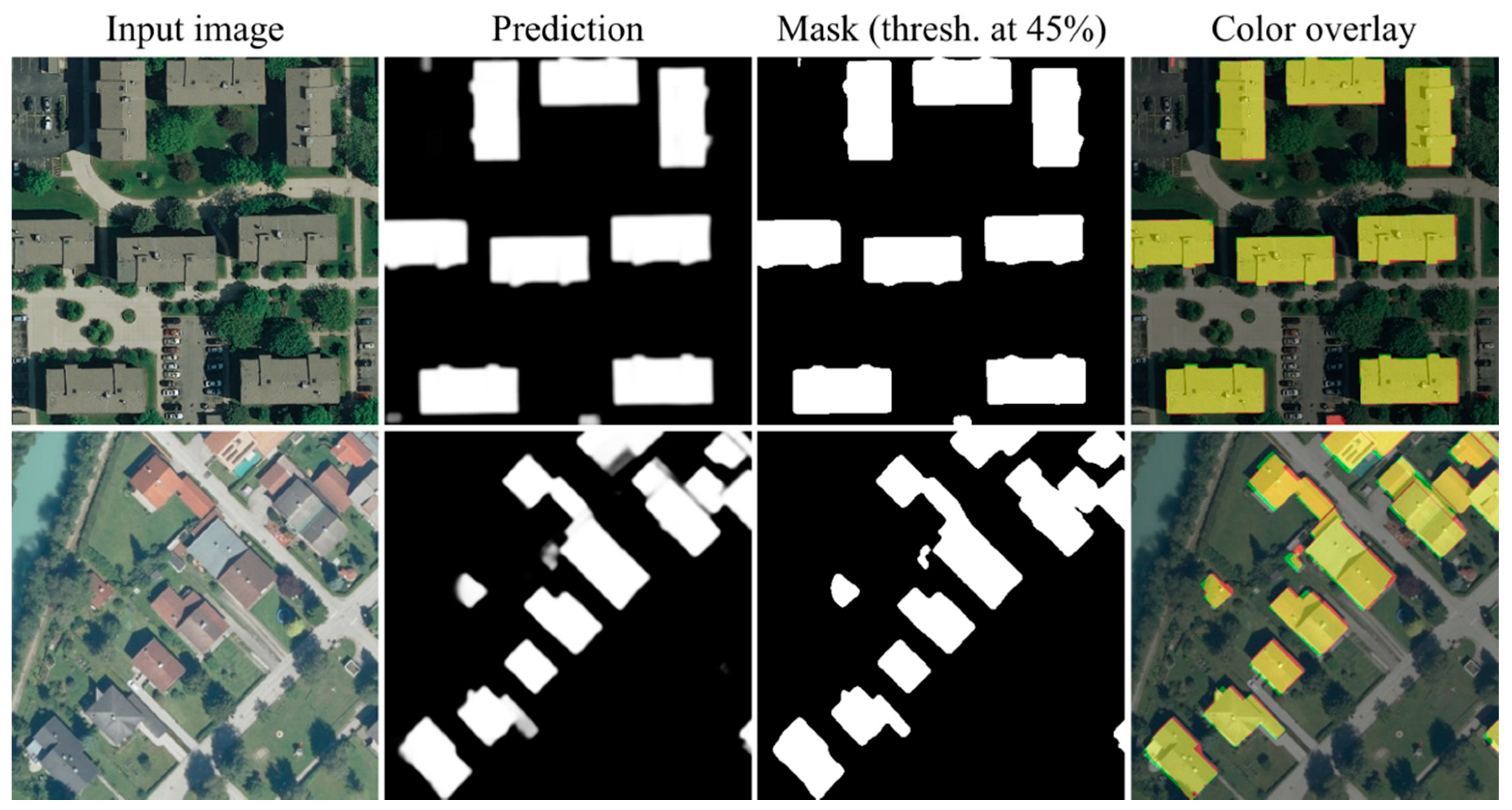
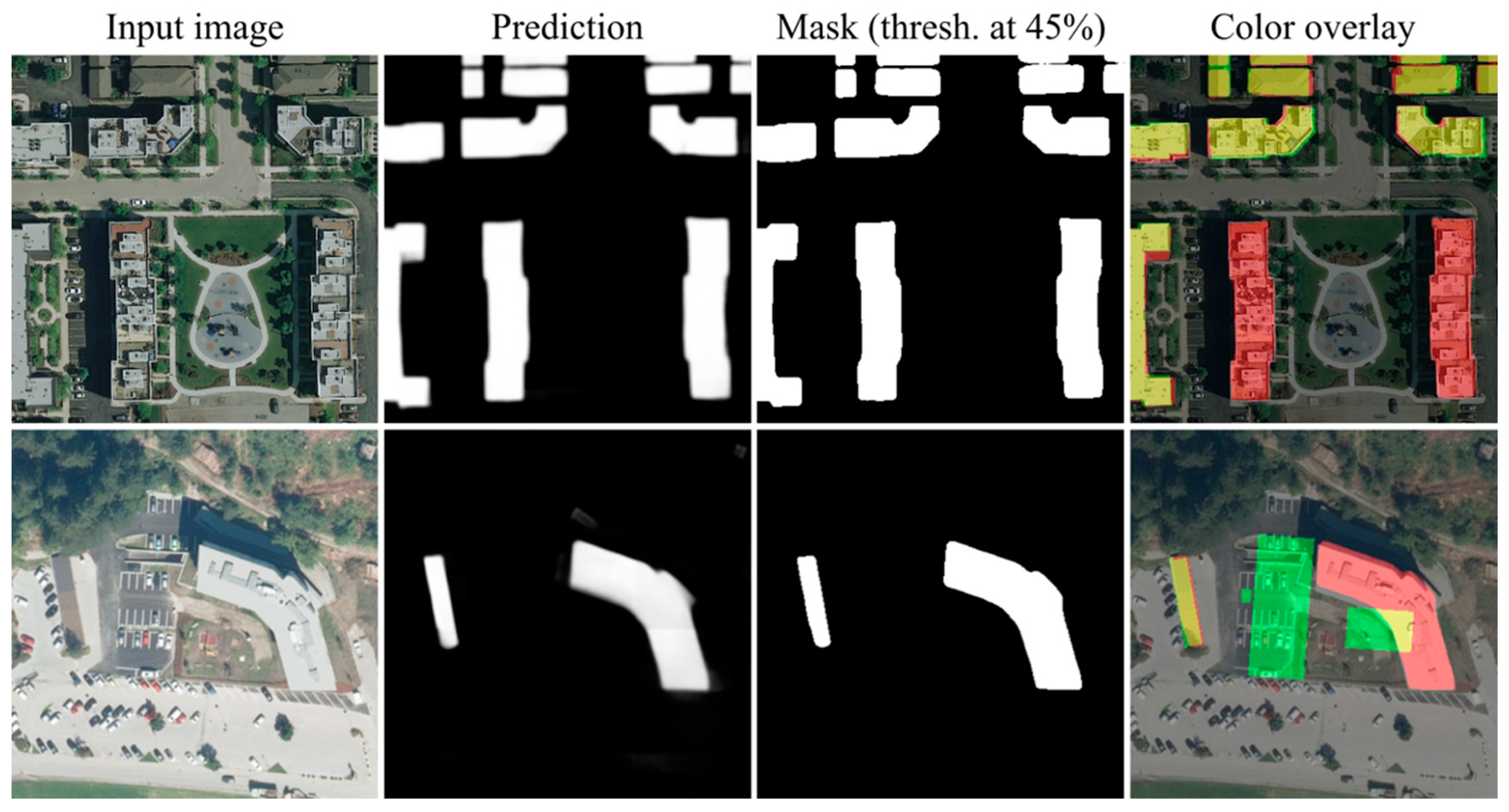
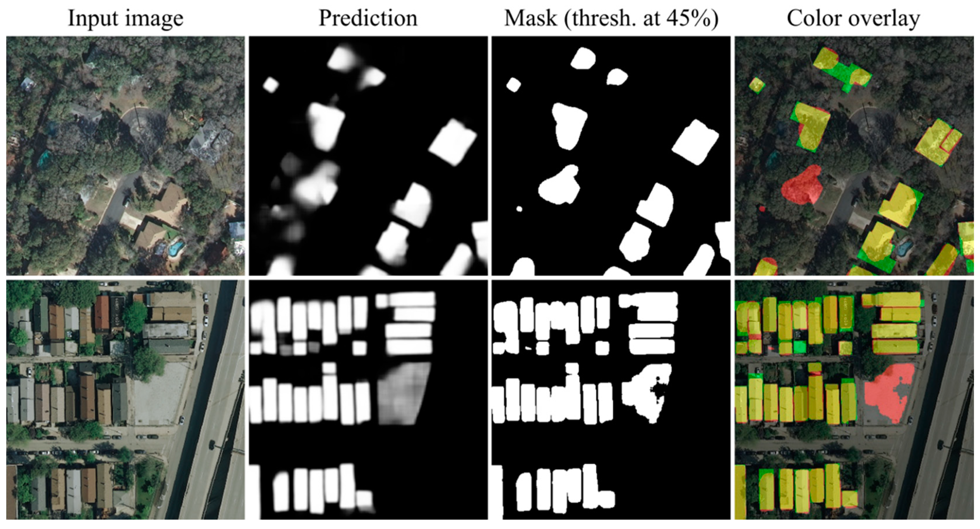
To gain more insight into the model behavior, for each image from the validation set that was used in the evaluation, we saved output predictions (grayscale images) and masks (threshold at 45%), so as the integral visualization that overlays output mask (in red) and ground truth mask (in green) over the input image. In locations where those two masks overlap, the resulting mask appears yellow. This visualization output allowed us to quickly detect areas where something went wrong by spotting red or green overlays in the image. In Figure 11, Figure 12 and Figure 13, we depicted several classes of examples found during overviewing previously explained visualizations. Each of these three figures shows a patch of the original input image, the obtained prediction, and mask, so as to show the appropriate visualization. The complete evaluation result can be found in ‘figshare.com’ [42].
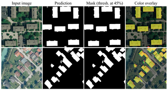
Figure 11.
Examples of correctly segmented buildings. The color overlay shows the obtained mask in red and the ground truth in green, resulting in a yellow overlay where those two overlaps.

Figure 12.
Examples of errors in the dataset that led to a mismatch between the output and the ground truth. The color overlay shows the obtained mask in red and the ground truth in green, resulting in a yellow overlay where those two overlaps.
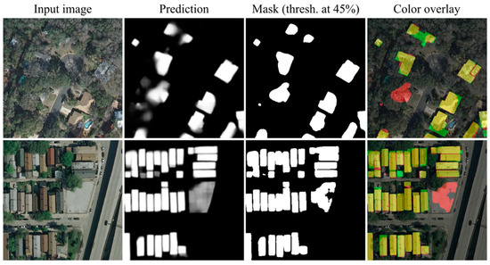
Figure 13.
Examples of segmentation errors. The color overlay shows the obtained mask in red and the ground truth in green, resulting in a yellow overlay where those two overlaps.
In Figure 11 we have the cleanest situation, i.e., it shows two examples where the output mask closely corresponds to the corresponding ground truth. Even in these two cases, the obtained segmentation mask is not pixel perfect, so some red and green pixels are present in the boundaries of the buildings.
The most interesting set of examples is shown in Figure 12. Here we have ‘segmentation errors’ that are actually due to invalid ground truth masks in the dataset. In the first example, we have two buildings that are correctly segmented, but the appropriate ground truth mask does not reflect the actual situation. In the second example, we have a case where two buildings are present in the ground truth mask (green rectangles), but the actual situation shows a completely different building that is also correctly segmented. Cases like these show us the potential application of the proposed method in validating ground truth information by automated processing of aerial imagery.
Finally, in Figure 13 we have two examples of real segmentation errors that come from the imperfection of the aerial images used for the given task, but also from the imperfection of the deep semantic segmentation model that is applied. In the first example, we have an area where most of the buildings are occluded with trees, so the model justifiably struggles to try to segment them. The uncertainty can be observed by looking at the prediction output. As a result, we have one significant false-positive example (red blob) while the rest of the buildings are segmented with high imprecision. The second example shows the model uncertainty about one possible building in the image (grayish area in the prediction) that resulted in some pixels slipping into the output mask (red blob) after thresholding.
Altogether, the conducted analysis shows the huge potential of the proposed approach. The question remains what could be achieved if we had a cleaner dataset, i.e., the dataset without mismatches between ground truth and the actual situation. This is important for both evaluation results, to provide more accurate metrics, but also for training so we do not mislead a model with false data and thus gain the better model.
6. Conclusions
In this paper, we proposed and evaluated an approach for building footprint extraction from aerial imagery using deep semantic segmentation. The building footprint extraction is considered as a special case, while the proposed approach can be used for many different tasks that require automated pixel-wise labeling of remote sensing imagery.
The method described in the paper can be conceived as a three-stage pipeline that consists of the following stages: image preparation, model implementation and training, and obtaining predictions. The image preparation stage deals with the problem of converting large input images to a format applicable for training. This stage also introduces the data augmentation technique appropriate for aerial images. The current model implementation relies on FPN segmentation architecture paired with ResNeXt-50 encoder, but as we already showed in the paper, other segmentation models are possible. Finally, the last stage deals with applying a trained ensemble of deep segmentation models to obtain predictions and final output masks. For that purpose, we used test-time augmentation (TTA) and weighted overlapping with the Gaussian kernel.
In the paper, we presented an evaluation of the proposed method, as well as the official contest results. The visual analysis of the evaluation results showed the particularly good ability of the model to accurately segment building footprints from the aerial imagery. It also showed many errors in the underlying dataset that consist of misalignment between ground truth masks and the actual situation. It also proved to be an efficient tool to detect such anomalies.
The potential application of automated building extraction would be to check if there are mismatches between buildings registered in some geodatabase and the actual situation depicted by satellite imagery. For future work, we intend to develop an automated method for detecting such areas by calculating local IoU metrics using a sliding window technique. Thresholding such an output, areas with low local IoU values could be identified suggesting a possible mismatch between ground truth and predicted mask. The appropriate information could be further used to fix the dataset ground truth, retrain the models, and compare results.
Author Contributions
Conceptualization, methodology, validation, formal analysis, supervision, writing, review and editing, data curation, Aleksandar Milosavljević. All authors have read and agreed to the published version of the manuscript.
Funding
This research received no external funding.
Acknowledgments
This study was supported by the Ministry of Education, Science and Technological Development, Republic of Serbia, as part of the projects III-43007 and III-47003.
Conflicts of Interest
The authors declare no conflict of interest.
References
- Zhang, Y.; Gong, W.; Sun, J.; Li, W. Web-Net: A Novel Nest Networks with Ultra-Hierarchical Sampling for Building Extraction from Aerial Imageries. Remote Sens. 2019, 11, 1897. [Google Scholar] [CrossRef]
- Lippitt, C.D.; Zhang, S. The impact of small unmanned airborne platforms on passive optical remote sensing: A conceptual perspective. Int. J. Remote Sens. 2018, 39, 4852–4868. [Google Scholar] [CrossRef]
- Yi, Y.; Zhang, Z.; Zhang, W.; Zhang, C.; Li, W.; Zhao, T. Semantic Segmentation of Urban Buildings from VHR Remote Sensing Imagery Using a Deep Convolutional Neural Network. Remote Sens. 2019, 11, 1774. [Google Scholar] [CrossRef]
- Gao, L.; Shi, W.; Miao, Z.; Lv, Z. Method Based on Edge Constraint and Fast Marching for Road Centerline Extraction from Very High-Resolution Remote Sensing Images. Remote Sens. 2018, 10, 900. [Google Scholar] [CrossRef]
- Mou, L.; Zhu, X.X. Vehicle Instance Segmentation from Aerial Image and Video Using a Multitask Learning Residual Fully Convolutional Network. IEEE Trans. Geosci. Remote Sens. 2018, 56, 6699–6711. [Google Scholar] [CrossRef]
- Nie, X.; Duan, M.; Ding, H.; Hu, B.; Wong, E.K. Attention Mask R-CNN for Ship Detection and Segmentation from Remote Sensing Images. IEEE Access 2020, 8, 9325–9334. [Google Scholar] [CrossRef]
- Li, W.; Hsu, C.Y. Automated terrain feature identification from remote sensing imagery: A deep learning approach. Int. J. Geogr. Inf. Sci. 2020, 34, 637–660. [Google Scholar] [CrossRef]
- Ye, Z.; Fu, Y.; Gan, M.; Deng, J.; Comber, A.; Wang, K. Building Extraction from Very High Resolution Aerial Imagery Using Joint Attention Deep Neural Network. Remote Sens. 2019, 11, 2970. [Google Scholar] [CrossRef]
- LeCun, Y.; Boser, B.; Denker, J.; Henderson, D.; Howard, R.; Hubbard, W.; Jackel, L. Handwritten digit recognition with a back-propagation network. In Advances in Neural Information Processing Systems; Papers NIPS. CC; MIT Press: Cambridge, MA, USA, 1990; pp. 396–404. [Google Scholar]
- Simonyan, K.; Zisserman, A. Very deep convolutional networks for large-scale image recognition. In Proceedings of the 3rd International Conference on Learning Representations, ICLR 2015—Conference Track Proceedings, San Diego, CA, USA, 7–9 May 2015. [Google Scholar]
- Maggiori, E.; Tarabalka, Y.; Charpiat, G.; Alliez, P. Can Semantic Labeling Methods Generalize to Any City? The Inria Aerial Image Labeling Benchmark. In Proceedings of the IEEE International Geoscience and Remote Sensing Symposium (IGARSS), Fort Worth, TX, USA, 23–28 July 2017; pp. 3226–3229. [Google Scholar]
- Castelluccio, M.; Poggi, G.; Sansone, C.; Verdoliva, L. Land Use Classification in Remote Sensing Images by Convolutional Neural Networks. Available online: http://arxiv.org/abs/1508.00092 (accessed on 27 January 2020).
- Marmanis, D.; Datcu, M.; Esch, T.; Stilla, U. Deep learning earth observation classification using ImageNet pretrained networks. IEEE Geosci. Remote Sens. Lett. 2016, 13, 105–109. [Google Scholar] [CrossRef]
- Srivastava, S.; Vargas Muñoz, J.E.; Lobry, S.; Tuia, D. Fine-grained landuse characterization using ground-based pictures: A deep learning solution based on globally available data. Int. J. Geogr. Inf. Sci. 2020, 34, 1117–1136. [Google Scholar] [CrossRef]
- Wojek, C.; Dorkó, G.; Schulz, A.; Schiele, B. Sliding-windows for rapid object class localization: A parallel technique. In Proceedings of the Lecture Notes in Computer Science (Including Subseries Lecture Notes in Artificial Intelligence and Lecture Notes in Bioinformatics), Munich, Germany, 10–13 June 2008; Volume 5096, pp. 71–81. [Google Scholar]
- Long, J.; Shelhamer, E.; Darrell, T. Fully Convolutional Networks for Semantic Segmentation. In Proceedings of the IEEE Conference on Computer Vision and Pattern Recognition (CVPR), Boston, MA, USA, 7–12 June 2015; pp. 3431–3440. [Google Scholar]
- Hariharan, B.; Arbeláez, P.; Girshick, R.; Malik, J. Hypercolumns for Object Segmentation and Fine-grained Localization. In Proceedings of the IEEE Conference on Computer Vision and Pattern Recognition (CVPR), Boston, MA, USA, 7–12 June 2015; pp. 447–456. [Google Scholar]
- Chen, L.C.; Papandreou, G.; Kokkinos, I.; Murphy, K.; Yuille, A.L. DeepLab: Semantic Image Segmentation with Deep Convolutional Nets, Atrous Convolution, and Fully Connected CRFs. IEEE Trans. Pattern Anal. Mach. Intell. 2018, 40, 834–848. [Google Scholar] [CrossRef] [PubMed]
- Noh, H.; Hong, S.; Han, B. Learning Deconvolution Network for Semantic Segmentation. In Proceedings of the IEEE International Conference on Computer Vision (ICCV), Santiago, Chile, 7–13 December 2015; pp. 1520–1528. [Google Scholar]
- Ronneberger, O.; Fischer, P.; Brox, T. U-Net: Convolutional Networks for Biomedical Image Segmentation. In Proceedings of the Lecture Notes in Computer Science (Including Subseries Lecture Notes in Artificial Intelligence and Lecture Notes in Bioinformatics); Springer: Cham, Switzerland, 2015; Volume 9351, pp. 234–241. [Google Scholar]
- Badrinarayanan, V.; Kendall, A.; Cipolla, R. SegNet: A Deep Convolutional Encoder-Decoder Architecture for Image Segmentation. IEEE Trans. Pattern Anal. Mach. Intell. 2017, 39, 2481–2495. [Google Scholar] [CrossRef] [PubMed]
- Kirillov, A.; He, K.; Girshick, R.; Dollár, P. A Unified Architecture for Instance and Semantic Segmentation. Available online: http://presentations.cocodataset.org/COCO17-Stuff-FAIR.pdf (accessed on 24 January 2020).
- Sun, G.; Huang, H.; Zhang, A.; Li, F.; Zhao, H.; Fu, H. Fusion of Multiscale Convolutional Neural Networks for Building Extraction in Very High-Resolution Images. Remote Sens. 2019, 11, 227. [Google Scholar] [CrossRef]
- Feng, Y.; Thiemann, F.; Sester, M. Learning Cartographic Building Generalization with Deep Convolutional Neural Networks. ISPRS Int. J. Geo-Inf. 2019, 8, 258. [Google Scholar] [CrossRef]
- Schuegraf, P.; Bittner, K. Automatic Building Footprint Extraction from Multi-Resolution Remote Sensing Images Using a Hybrid FCN. ISPRS Int. J. Geo-Inf. 2019, 8, 191. [Google Scholar] [CrossRef]
- Xu, Y.; Wu, L.; Xie, Z.; Chen, Z. Building Extraction in Very High Resolution Remote Sensing Imagery Using Deep Learning and Guided Filters. Remote Sens. 2018, 10, 144. [Google Scholar] [CrossRef]
- Guo, R.; Liu, J.; Li, N.; Liu, S.; Chen, F.; Cheng, B.; Duan, J.; Li, X.; Ma, C. Pixel-Wise Classification Method for High Resolution Remote Sensing Imagery Using Deep Neural Networks. ISPRS Int. J. Geo-Inf. 2018, 7, 110. [Google Scholar] [CrossRef]
- Xie, Y.; Cai, J.; Bhojwani, R.; Shekhar, S.; Knight, J. A locally-constrained YOLO framework for detecting small and densely-distributed building footprints. Int. J. Geogr. Inf. Sci. 2020, 34, 777–801. [Google Scholar] [CrossRef]
- Inria Aerial Image Labeling Dataset. Available online: https://project.inria.fr/aerialimagelabeling/ (accessed on 11 August 2020).
- Keras: The Python Deep Learning Library. Available online: https://keras.io (accessed on 24 January 2020).
- TensorFlow: An End-To-End Open Source Machine Learning Platform. Available online: https://www.tensorflow.org/ (accessed on 24 January 2020).
- Milosavljević, A. Inria Aerial Image Labeling—Building Footprint Extraction Using Deep Semantic Segmentation. Available online: https://github.com/a-milosavljevic/inria-aerial-image-labeling (accessed on 11 August 2020).
- Yakubovskiy, P. Segmentation Models, Github Library. Available online: https://github.com/qubvel/segmentation_models (accessed on 24 January 2020).
- Chaurasia, A.; Culurciello, E. LinkNet: Exploiting encoder representations for efficient semantic segmentation. In Proceedings of the 2017 IEEE Visual Communications and Image Processing, VCIP 2017, St. Petersburg, FL, USA, 10–13 December 2017; pp. 1–4. [Google Scholar]
- Zhao, H.; Shi, J.; Qi, X.; Wang, X.; Jia, J. Pyramid Scene Parsing Network. In Proceedings of the IEEE Conference on Computer Vision and Pattern Recognition (CVPR), Honolulu, HI, USA, 21–26 July 2017; pp. 2881–2890. [Google Scholar]
- He, K.; Zhang, X.; Ren, S.; Sun, J. Deep residual learning for image recognition. In Proceedings of the IEEE Conference on Computer Vision and Pattern Recognition, Las Vegas, NV, USA, 27–30 June 2016; pp. 770–778. [Google Scholar]
- Hu, J.; Shen, L.; Sun, G. Squeeze-and-Excitation Networks. In Proceedings of the IEEE Conference on Computer Vision and Pattern Recognition (CVPR), Salt Lake City, UT, USA, 18–23 June 2018; pp. 7132–7141. [Google Scholar]
- Xie, S.; Girshick, R.; Dollár, P.; Tu, Z.; He, K.; San Diego, U. Aggregated Residual Transformations for Deep Neural Networks. In Proceedings of the IEEE Conference on Computer Vision and Pattern Recognition (CVPR), Honolulu, HI, USA, 21–26 July 2017; pp. 1492–1500. [Google Scholar]
- Sudre, C.H.; Li, W.; Vercauteren, T.; Ourselin, S.; Jorge Cardoso, M. Generalised dice overlap as a deep learning loss function for highly unbalanced segmentations. In Proceedings of the Lecture Notes in Computer Science (Including Subseries Lecture Notes in Artificial Intelligence and Lecture Notes in Bioinformatics); Springer: Cham, Switzerland, 2017; Volume 10553, pp. 240–248. [Google Scholar]
- Hinton, G.; Srivastava, N.; Swersky, K. Neural Networks for Machine Learning, Lecture 6a Overview of Mini-Batch Gradient Descent. Available online: http://www.cs.toronto.edu/~hinton/coursera/lecture6/lec6.pdf (accessed on 24 January 2020).
- Jordan, J. Setting the Learning Rate of Your Neural Network. Available online: https://www.jeremyjordan.me/nn-learning-rate/ (accessed on 24 January 2020).
- Milosavljević, A. Building Footprint Extraction Using Deep Semantic Segmentation. Figshare. Figure. Available online: https://doi.org/10.6084/m9.figshare.11816616.v1 (accessed on 11 August 2020).
© 2020 by the author. Licensee MDPI, Basel, Switzerland. This article is an open access article distributed under the terms and conditions of the Creative Commons Attribution (CC BY) license (http://creativecommons.org/licenses/by/4.0/).

