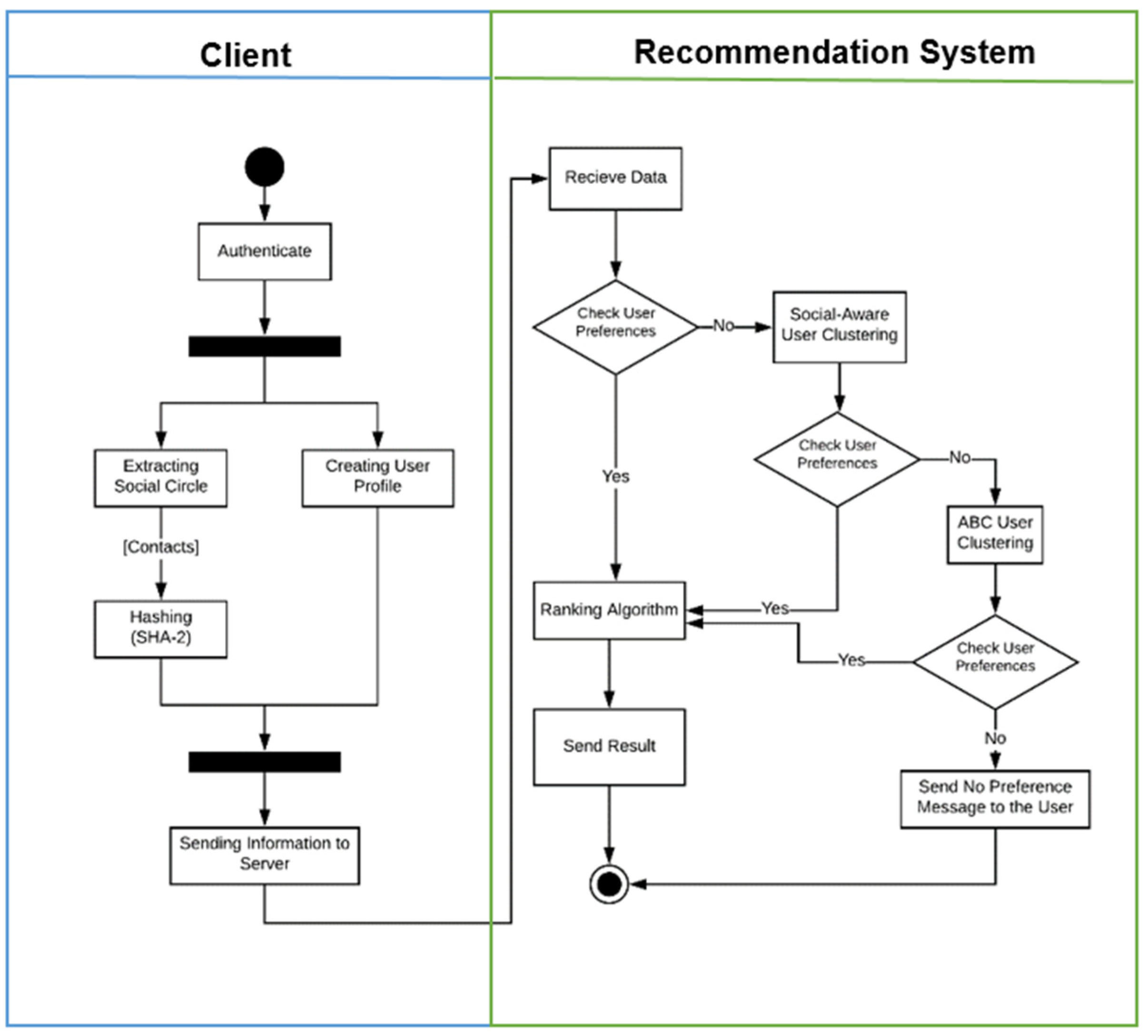
Another challenge here is how to use a USDE while protecting user’s privacy. Although detailed user privacy research needs to be conducted especially on resource-restrained devices such as cellphones, in this paper we used user profile anonymization to support user’s privacy. The user’s ID and profile are shared using a secure hash algorithms (SHA)-512 approach for the user’s social circle. USDE utilizes a list of user profiles (with a constantly updated list) with hashed user IDs in the process of making recommendations. Using an anonymization technique, the user profiles and their social circles are delivered without users’ real identity information in the case of user similarity clustering. In this way, their identity remains anonymous on the server while similar user profiles can be used in the proposed RS.
4.1. Social Interaction Classification
The similarity between users can be identified by analyzing their social interactions such as emails, call logs, and bidirectional social relationships extracted from SNs. Inspired by Elsesser and Peplau [
48], social interactions between users can be categorized into two different categories due to the strength of bonds existing in their social interactions. The first category is called primary social interactions (PSIs), that includes real-world relationships between users such as making a call and sending or receiving messages and emails. The number of members placed in the group of similar users with PSIs is usually small and characterized by extensive and real-world interactions between group members on a regular basis. The second category is called secondary social interactions (SSIs) includes interactions made in the virtual world such as relationships between users on social networking sites such as Facebook. Similar users with SSIs can be characterized by almost larger numbers of members and more impersonal and virtual interactions.
Using this classification, users placed in the social circle of the target user can be seen as a group of similar users with PSIs or SSIs. The social circle of the target user is created from the contact list of the user’s smartphone, list of the user’s friends in SNs, senders and receivers of emails and text messages. The frequency and number of times that a user contacts the target user can define the strength of bonds existing in their social interactions. Although the social interaction can be further expanded in future research, in this paper, we considered only two categories (i.e., PSI and SSI) based on the frequent contact concept. If a person in the social circle of the target user contacts him/her more than once a week; then, the RS considers this person as a user with PSIs with the target user. After the labeling of target user’s PSIs, the rest of the target user’s social circle are classified as users with SSIs. As an example, consider the situation that {u1, u2, u3, u4} is extracted as the social circle of the target user X. If u2 has made a phone call to the user X three times a week, and u3 frequently sent an email to the user X last week, then, u2 and u3 are classified as the target user X’s PSIs. While u1 and u4 are labeled as users with SSIs.
It is assumed in this paper that the similarity between the target user and users with PSIs is greater than the similarity of users with SSIs. It appears obvious that the recommendations made by people who are in the group of similar users with PSIs would be considered more reliable than those made by the group of similar users with SSIs. Based on this assumption, we consider the trust in the recommendations made by the group of similar users with PSIs as being twice as much as those from the group of similar users with SSIs. However, if we don’t have a significant number (i.e., 30 [
49]) of people in the social circle, the user clustering method is used and the trust weight is considered 1 again. Hence, the trust weights are considered as follows:
This trust weight can be used in computing the average rating for the new user based on the other similar users. The trust weight of the group of similar users with PSIs is set to twice as much as those from the group of similar users with SSIs for this paper, however, this value can be modified by users if they want to trust their social contacts more than their group of similar users. If the target user has two users and in his/her social circle of similar users with SSIs and PSIs respectively, the effect of the trust weight on their recommendation can be measured. Consider the case that user and gave ratings 4 and 5 to item and the trust weight is set to 3 instead of 2 for users with PSIs, here the user . In this situation, the final recommendation will be 9% closer to the rating given by user compared to that given in the situation that the trust weight has been set to 2 for users with PSIs. This value is 6% more than the rating from user in situation that the trust weight is set to 1.5 instead of 2 for users with PSIs.
4.2. User Profile Clustering
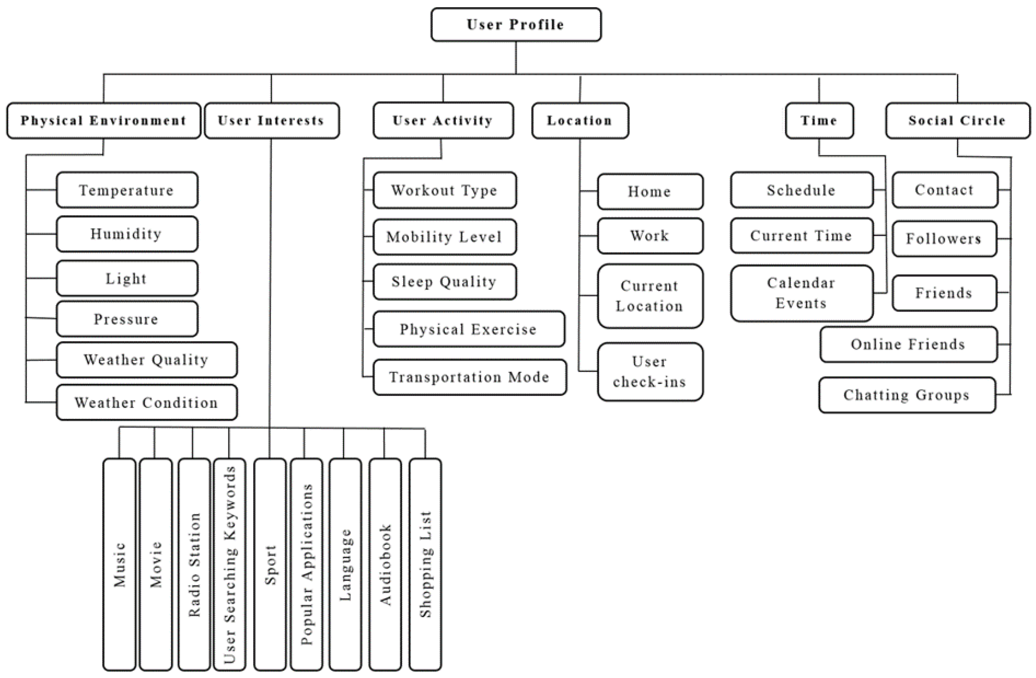
A variety of attributes can be included in the user profile to describe a user as context information. The greater the number of profile attributes, the better the understanding of the user. When the CSP occurs, finding implicit similarities between users addresses profile matching and user clustering. User profile clustering is an analytic process designed to explore users by discovering consistent patterns and/or systematic relationships between contexts, and then validate the findings by applying the detected patterns to new subsets of users. Generally, clustering algorithms can be categorized into partitioning methods, hierarchical methods, density-based methods, grid-based methods, and model-based methods. An excellent survey of clustering techniques can be found in a study done by Kameshwaran et al. [
50].
Given a data set where is a pattern in the –dimensional feature space, and is the number of patterns in , then the clustering of is the partitioning of into clusters that satisfies the following conditions:
Each pattern should be assigned to a user cluster, i.e., .
Each user cluster has at least one context pattern assigned to it, i.e., .
Each context pattern is assigned to one and only one user cluster, i.e., .
Clustering is the process of identifying clusters of users within multidimensional user profile data (contexts) based on feature space (i.e., user profile items) through similarity measure. The most popular way to evaluate a similarity measure is through the use of distance measures [
51]. The most widely used distance measure is the Euclidean distance, defined as:
Recently, a huge increase in the use of Swarm-based optimization techniques for clustering has been observed [
52]. Swarm Intelligence is an innovative distributed intelligent paradigm for solving optimization problems that were originally inspired by the biological examples of the swarming, flocking, and herding phenomena in vertebrates [
53]. These techniques incorporate swarming behaviors observed in flocks of birds, schools of fish, swarms of bees, or even human social behavior, from which the idea emerged [
54,
55,
56]. They can also be used especially when other methods are too expensive or difficult to implement [
57]. For clustering of massive user profile data, we used artificial bee colony (ABC) algorithm because of its potential in solving complex optimization problems, flexibility, simplicity, self-organizing and extensibility [
53,
58]. To evaluate the performance of ABC, its performance is compared with K-means as a popular clustering algorithm in data mining [
51].
A colony of honey bees can spread itself out over long distances to exploit a large number of food sources [
53]. The foraging process begins in a colony by scout bees sent to search for promising flower patches. Flower patches with large amounts of nectar or pollen that can be collected with less effort tend to be visited by more bees, whereas patches with less nectar or pollen receive fewer visits from bees [
57]. The artificial swarm bee colony clustering method exploits the search capability of the bee algorithm to overcome the local optimum problem of the
–means algorithm. More specifically, its task is to search for the appropriate cluster centers (
,
,…,
) so that the clustering metric
(2) is minimized. The basic steps of this clustering operation are listed in the
Table 4.
In the initialization stage (Step 1 in
Table 4), a set of scout bee population (
) is randomly selected to define the
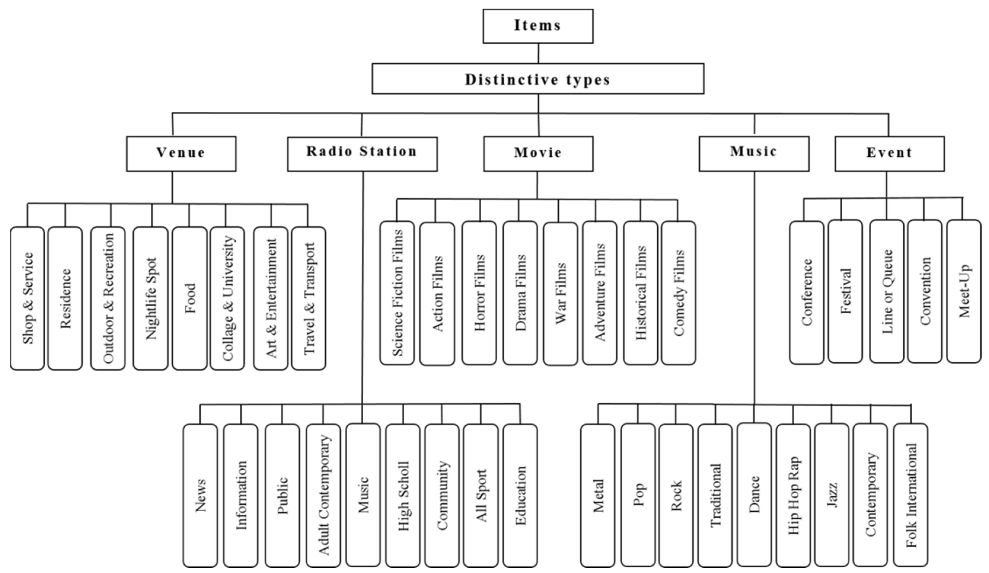
clusters. The Euclidean distances between each user profile data pattern and all centers are calculated to determine the assigned cluster to each user profile. For example, in the case of the movie RS, user profile items such as movie genres and social circles are considered for the clustering. This way, initial clusters can be constructed. After the clusters have been formed, the original cluster centers are replaced by the actual centroids of the clusters to define a particular clustering solution
i.e., a bee). This initialization process is applied each time new bees are created.
In Step 2 of
Table 4, the fitness computation process is carried out for each site visited by a bee by calculating the clustering metric
(2), which is inversely related to fitness.
Step 3 is the main step of bee colony optimization, which starts by forming a new population (Step 3a). In Step 3b, sites with the highest fitness are designated as “selected sites” and chosen for the neighborhood search. In Steps 3c and 3d, the algorithm conducts searches around the selected sites, assigning more bees to search in the area of the best sites. Selection of the best sites can be made directly according to their associated fitness. Alternatively, the fitness values are used to determine the probability of the sites being selected. Searches in the neighborhood of the best sites—those that represent the most promising solutions—are carried out in greater detail. As mentioned previously, this is done by recruiting more bees for the best sites than for the other selected sites. Together with scouting, this differential recruitment is a key operation of the bee algorithm. In Step 3d, only the bee that has found the site with the highest fitness (i.e., the “fittest” bee) will be selected to form part of the next bee population. In nature, there is no such restriction. The restriction is introduced here to reduce the number of points to be explored. In Step 3e, the remaining bees in the population are randomly assigned to the search space to scout for new potential solutions.
At the end of each loop, the colony will have two parts to its new population: representatives from the selected sites, and scout bees assigned to conduct random searches. These steps are repeated until the stopping criterion is met.
Each bee represents a potential user similarity clustering solution as a set of
cluster centers, and each site represents the patterns or user profile data objects. The algorithm requires some parameters to be set, namely: number of scout bees (
), number of sites selected for neighborhood searching (
), number of top-rated (
) sites among
selected sites (
), number of bees recruited for the best
sites (
), number of bees recruited for the other (
) selected sites (
), and the stopping criterion for the loop. In the
Table 5, the list of initial values for the parameters are presented.
For the presented user dataset (
Section 6), each of the ABC and
-means algorithm is applied 30 times individually to a random initial solution. The parameters of all the algorithms are set as per
Table 5. The sum of the intra-cluster distances, i.e., the distances between the data vectors within a cluster and the centroid of this cluster, as defined in (2), are used to measure the quality of a clustering. Clearly, the smaller the sum of the distances, the higher the quality of clustering. The effectiveness of stochastic algorithms is greatly dependent on the generation of the initial solutions. For every dataset, algorithms performed their own effectiveness tests 30 times individually, each time with randomly generated initial solutions. The values reported are the averages of the sums of intra-cluster distances and the fitness values of the worst and best solutions which can indicate the range of values that the algorithms span.
Table 6 summarizes the intra-cluster distances and performance time on the server obtained from all the algorithms for the data sets above.
From the values in
Table 6, we can conclude that the results obtained by ABC outperforms a
-means clustering algorithm in both accuracy and the average time (number of iteration steps). A sample distribution in user clustering by the ABC algorithm is shown in
Figure 3 in which the social circle cluster graphs are represented by lines. As seen from the
Figure 3, cluster heads are uniformly selected by the ABC algorithm provided that clusters have regions that are approximately equal in size.


