Abstract
In this paper, we examine a buffer with active management that rejects packets basing on the buffer occupancy. Specifically, we derive several metrics characterizing how effectively the algorithm can prevent the queue of packets from becoming too long and how well it assists in flushing the buffer quickly when necessary. First, we compute the probability that the size of the queue is kept below a predefined level L. Second, we calculate the distribution of the amount of time needed to cross level L, the buffer overflow probability, and the average time to buffer overflow. Third, we derive the distribution of the amount of time required to flush the buffer and its average value. A general modeling framework is used in derivations, with a general service time distribution, general rejection function, and a powerful model of the arrival process. The obtained formulas enable, among other things, the solving of many design problems, e.g., those connected with the design of wireless sensor nodes using the N-policy. Several numerical results are provided, including examples of design problems and other calculations.
1. Introduction
Active queue management (AQM) in a packet buffer is a policy which assumes that an arriving packet may be deleted upon arrival instead of being deposited in the buffer, even if there is an unoccupied space in the buffer. There are several good reasons why AQM may be recommended in packet networking. Its main purpose, however, is always to reduce queue sizes in buffers and thus reduce the latencies induced by buffering mechanisms.
Obviously, the packet delivery time is of importance in all sorts of networks. Therefore, AQM is recommended by researchers and engineers for wired networks [1,2], wireless sensor networks [3,4,5], LTE and 5G networks [6,7], mobile ad hoc networks [8,9], satellite networks [10,11], and others.
The primary purpose of this paper is to examine the effectiveness of the AQM mechanism in maintaining a short queue.
In this paper, we adopt a popular type of AQM in which packets are deleted randomly based on the buffer occupancy.
This type of AQM is depicted in Figure 1. In detail, upon the arrival of a packet at the buffer, a random decision is made (using an RNG) as to whether this packet should be deposited in the buffer or deleted. Specifically, with probability , the packet is deleted, where i denotes the current queue size (see Figure 1).
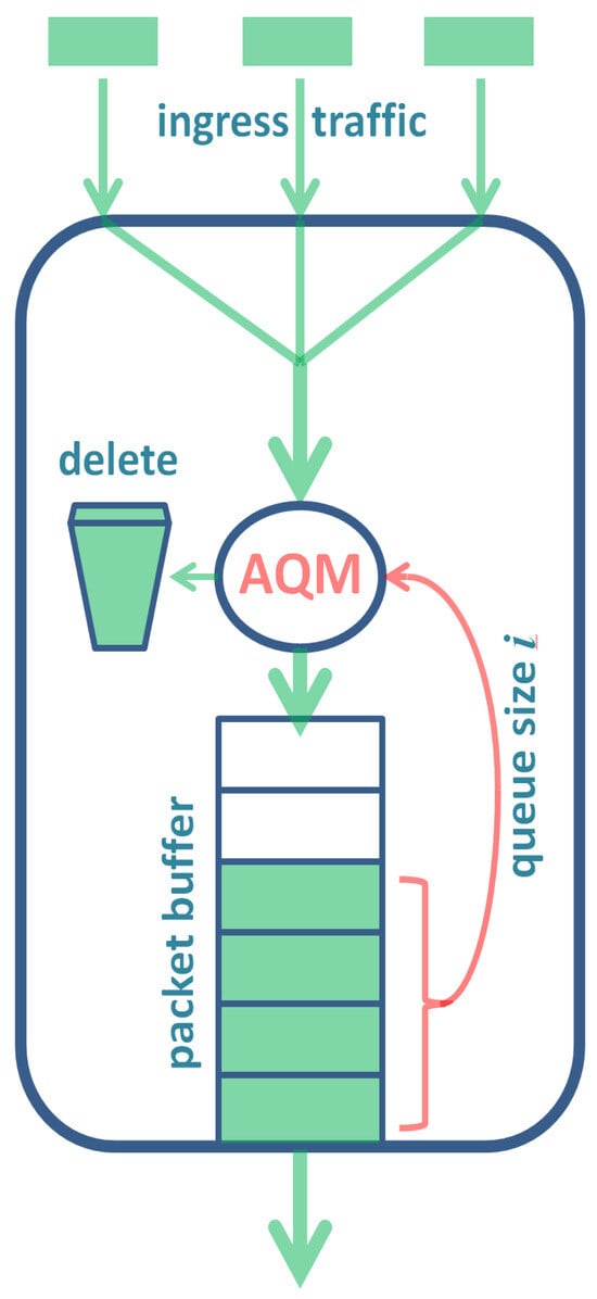
Figure 1.
Buffer with AQM based on the queue size.
In the literature, many types of function are used in AQM, e.g., linear [12], quadratic [13], sinusoidal [14], cubic [15,16], exponential [17], beta [18], and Gaussian functions [9]. Additionally, some researchers propose in a combined form, consisting of two linear functions [19], linear and quadratic functions [20], linear and cubic functions [21], linear and exponential functions [22], or quadratic and exponential functions [23]. Herein, we adopt function in a general form. Therefore, all of the results will be applicable to all particular forms of listed in the previous paragraph, and any others.
It should be mentioned that AQM, based solely on the function , is not the only possible approach. For instance, in [24], the packet sojourn time through the buffer is used for calculating the rejection probability. In [25], a compensated proportional–integral–derivative (PID) controller, based on queuing latency, is exploited, while [25] uses different update times than the -based method. Specifically, the rejection probability is updated at regular time intervals, rather than upon the arrival of packets, as is the case in the method. In the algorithm from [26], a virtual queue is maintained with a capacity smaller than the capacity of the actual link. The actual and virtual queues are both updated upon the arrival of a packet, but the packet is rejected when the virtual, rather than actual, buffer overflows. In [27], a proportional–derivative (PD) controller, accompanied by a Smith predictor and disturbance observer mechanism, is used. Finally, in [28,29], neural networks and fuzzy logic are exploited in the design of the AQM algorithm, respectively.
The popularity of the -based method in AQM studies is connected with the fact that it provides a good trade-off between the performance of the algorithm and the difficulty of implementation in a real networking device. Specifically, the -based method usually offers a substantial improvement when compared with no AQM at all while remaining relatively easy to implement. This was confirmed by the experimental study in [30], where such an algorithm was implemented in a real device and tested in a real network.
In this paper, we will check how well an AQM algorithm based on the function can maintain a short queue of packets.
To achieve this, we will first derive the probability that the size of the queue is kept below some level L (see Figure 2), using a queuing model of the buffer with AQM. Naturally, the longer we wait, the higher the probability of hitting L. Therefore, we derive the probability of not hitting L within a concrete time interval , as illustrated in Figure 2.
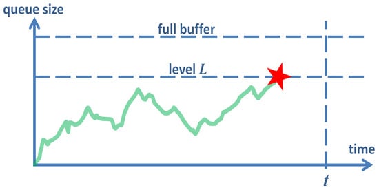
Figure 2.
Queue size evolution and the event of hitting level L.
Then, we will derive several other characteristics connected with level crossing. These include the distribution of the duration of time before which the size of the queue reaches level L (i.e., the time to the red event in Figure 2) and its average value. Naturally, the longer the average amount of time needed to hit L, the better AQM is performing in terms of keeping the queue short.
In the characteristics mentioned so far, L is not specified, i.e., an arbitrary L can be used depending on particular needs. Therefore, we can also use , where B is the size of the buffer. For such L, we will obtain buffer overflow characteristics, i.e., the probability of no buffer overflows in a given interval, the distribution of the time to overflow, and the average time to buffer overflow.
Obviously, all of the level-crossing characteristics depend on three components of the queuing model: the statistical properties of traffic arriving at the buffer, the capacity of the output link, and the type and parameterization of AQM. All three of these components are highly general in the model studied here, which translates into broad applicability of the results to many different scenarios.
First, a powerful model of the arrival process is adopted, one which can mimic an arbitrary distribution of time between consecutive packets and features an autocorrelated structure of traffic, batch arrivals of packets, and several other statistical features. Second, a general type of distribution of the transmission time is used. It may model various packet transmission times (attributed to various packets), a dynamically changing link capacity (e.g., due to the wireless environment), or both.
In addition to the characteristics described above reflecting the tendency of the queue size to grow, we will derive characteristics reflecting the tendency of the queue size to decrease when the transmission rate is high. Namely, we will find formulas for the distribution of the amount of time required to flush the buffer and the average amount of required time to flush the buffer, as illustrated in Figure 3.

Figure 3.
Time to flush the buffer.
1.1. Application Scenarios
The aforementioned level-crossing characteristics have many potential applications.
For instance, several application scenarios are associated with the design of wireless sensor networks (WSNs) incorporating an energy-saving mechanism based on the N-policy. This policy has been recommended for WSNs, for example, in [31,32,33,34,35,36].
Specifically, a wireless sensor node that utilizes the N-policy has its radio output interface switched off part of the time to conserve energy in the battery. This interface is activated only when the number of packets in the buffer reaches a critical level. The node then transmits packets until the buffer becomes empty, after which the output interface is deactivated again, and the process repeats. In Figure 4, the model of a sensor node using the N-policy, as considered here, is depicted. It differs from the original proposition of the N-policy (see Figure 1 in [31]) due to the inclusion of the AQM mechanism, which is an additional component here.
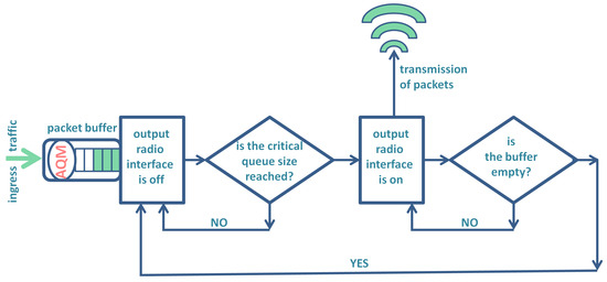
Figure 4.
Model of a sensor node incorporating the N-policy and AQM.
When designing a sensor node with the N-policy, we may encounter several problems. For instance, we may need to calculate how much energy is consumed by the output radio in one buffer flush cycle, as depicted in Figure 3. This energy is obviously proportional to the buffer flush time, which is one of the characteristics derived here.
Next, we may need to calculate the average energy consumption of the output radio over an extended period, considering alternating active and idle periods along with their respective proportions. The active period corresponds to the buffer flush time discussed above. The idle period represents the time during which the queue size increases from 0 to the critical level L, as depicted in Figure 2. This is another level-crossing characteristic derived here.
Finally, instead of computing the buffer flush time for given system parameters, we may search for system parameters (e.g., AQM parameters, transmission rate) that yield an assumed a priori flush time.
Examples of solutions for such problems are presented in Section 4.1.
1.2. Contribution
In summary, the contribution of the paper consists of several new formulas, specifically formulas for
- the probability that the size of the queue is below L in , Formula (26);
- the probability that the buffer is not overflowed during , Formula (38);
- the distribution of the amount of time needed to flush the buffer, Formula (52);
- the average amount of time needed to flush the buffer, Formula (57);
These formulas were obtained for a model of the AQM buffer with high generality, a powerful traffic model, general duration of the transmission time, and an AQM mechanism with the function in the general form.
Furthermore, several numerical examples are provided, illustrating all of the aforementioned level-crossing characteristics and their dependence on system parameters, as well as examples of solutions to design problems. A few such solutions are shown in Section 4.
As far as the author knows, the results of this paper are new.
Active queue management, which rejects packets basing on the buffer occupancy, was recommended in [9,12,13,14,15,16,17,18,19,20,21,22,23]. However, all of these studies are based on simulations rather than on queuing theory. They focus mostly on the influence of the particular form of the rejection function (linear, cubic, exponential, etc.) on the buffering mechanism. Typically, the queue size and packet loss were studied, while the level-crossing characteristics were not determined. Herein, we study the level-crossing characteristics using a queuing model which encompasses all of the mentioned particular rejection functions.
On the other hand, the level-crossing characteristics were investigated in several other papers using methods of queuing theory, [37,38,39,40,41,42,43]. Unfortunately, all of the models from [37,38,39,40,41,42,43] lack the active management component, which is central here. The AQM component is also absent in all the studies conducted so far on models of a sensor node with the N-policy, [31,32,33,34,35,36].
Next, there are many published papers in which a model incorporating active management is studied mathematically, e.g., [44,45,46,47,48,49,50]. However, in none of these papers are the level-crossing characteristics analyzed.
Some level-crossing characteristics in a model of an actively managed buffer were studied in [51]. Unfortunately, the analysis in [51] was based on a very simple model of the arrival process, i.e., without autocorrelation, batch arrivals, and other advanced features. The model considered herein incorporates autocorrelation and group (batch) arrivals. As shown in the numerical results, autocorrelation exerts a tremendous effect on the level-crossing characteristics. Furthermore, it is known that networking traffic is very often autocorrelated, [52], so this feature of the model is of great practical importance. It also complicates the analysis.
Finally, in [24,25,26,27,28,29], we can find examples of AQM algorithms which are based on factors other than buffer occupancy.
The rest of the paper is organized as follows. In Section 2, the queuing model is defined, including the input traffic model and AQM mechanism. Moreover, the notation of model parameters is introduced. In Section 3, the level-crossing characteristics are derived. This section is divided into Section 3.1, Section 3.2, Section 3.3 and Section 3.4, in which the probability that the size of the queue is below L, distribution of the duration of time to hit level L, buffer overflow characteristics, and buffer flush characteristics are obtained, respectively. Numerical results are shown in Section 4. They are based on two traffic parameterizations, several target levels L, variable service rates, and variable AQM parameters. Closing remarks are gathered in Section 5.
2. Modeling Framework
We deal with the model of a FIFO buffer equipped with active queue management basing on the function, as shown in Figure 1.
Specifically, packets arrive at the buffer according to a complex arrival process, which will be described below. They line up in the buffer in the same order they arrived. The capacity of this buffer is B packets, which includes the head position for the packet currently being transmitted.
If the buffer is saturated, every new packet is deleted upon arrival. Moreover, every other packet may be deleted upon arrival, even if there is still some space in the buffer. Such deletion is performed by the active management mechanism randomly, based on an RNG. Specifically, each arriving packet is deleted with probability or put into the buffer with probability , where i is the buffer occupancy upon its arrival.
Simultaneously, the queue of packets is drained from the buffer by the output transmission link. The transmission of a packet takes a random amount time, which has the distribution function . In such a model, the changeability of the transmission time can be attributed to the changeability of the packet size or the changeability of the physical link capacity, or both.
Functions and are not specified and may have any form provided they fulfill the obvious assumptions, i.e., for every i and for .
The average service time will be denoted by .
The packet arrival process is modeled by the batch Markovian arrival process, [53]. This process has a very rich statistical structure and possesses powerful modeling possibilities. In particular, it was shown that it can simultaneously model an arbitrary interarrival period and arbitrary autocorrelation structure, [54]. It enables modeling of the batch structure of traffic, which is induced by some networking protocols, as discussed in [55]. It is also able to model many other subtle properties of packet traffic.
The most popular parameterization of the batch Markovian process has the form of the sequence , where each is an matrix. This sequence can be infinite if the length of an arriving batch can be arbitrarily large. In practice, very often this sequence is finite, i.e., has the form , where N is the maximum possible batch size in the process of interest. Herein, we assume the most general case, with an unlimited batch size.
Sequence must fulfill the following requirements:
- is non-negative for , is non-negative except for the diagonal;
- must have all rows summing to zero;
- .
In this notation, D is the rate matrix of the modulating Markov chain, with state space . The evolution of this modulating chain (of continuous type) controls arrivals of packets, perhaps in batches. In particular, if the modulating chain assumes state i at some moment in time, then for an exponentially distributed epoch with rate , nothing happens. After that time, either the modulating state changes, a batch arrives, or both. The rate is equal to the modulus of the i-th diagonal entry of matrix .
The total rate of such arrival process, , is equal to
where
and denotes the stationary distribution of the Markov chain, which can be calculated by solving the system
The rate of arrivals of groups (batches) is then
The variance of interarrival times equals
while the k-lag autocovariance of interarrival times, C, is
where
and distribution can be obtained from the linear system
Now, having (6) and (7), we can calculate the k-lag autocorrelation of interarrival times, , which equals
has a tremendous effect of various buffering characteristics. Herein, in Section 4, we will see its profound impact on the level-crossing characteristics. Importantly, in the batch Markovian arrival process, can be modeled arbitrarily (see, e.g., [54]).
Other important properties and characteristics of the batch Markovian arrival process may be found by the reader in [56].
Basic characteristics of queues with the batch Markovian arrival process (but no AQM) can be found in [56,57].
In the analysis, we will need two special characteristics of the model, and .
In particular, denotes the probability that v packets are deposited in the buffer before time t and that the modulating state at t is j; assuming that no packet transmission is finished by t, the initial buffer occupancy (i.e., at ) was k, whereas the initial modulating state was i. Hence, this characteristic describes the raw effect of the AQM mechanism on the arrival process in interval , excluding the impact of the service process.
The second characteristic, , denotes the probability that if u packets arrive as a batch, v of them are deposited in the buffer, whereas the rest are deleted, assuming the buffer occupancy was k upon this arrival. Therefore, this characteristic describes the instant impact of the AQM mechanism on the batch of arriving packets, if the packets arrive in a batch.
It will be revealed in the next section how and can be computed.
3. Level-Crossing Characteristics
3.1. Probability That the Queue Is Below L
Let denote the probability that in interval the size of the queue is under L, given that initially the queue was of size k and that the initial modulating state was i, where and .
If , then the following equation holds:
Equation (11) is acquired by conditioning upon the first transmission completion time, y, which is distributed according to F.
The first segment of (11) is devoted to the event . In this event, v new packets are deposited in the buffer by the time y and the new modulating state at time y is j. To assure that level L is not hit, it must hold . Taking into account the transmission completed at y, the new buffer occupancy at y is . Thus at y, the conditional probability of no hitting L by t is .
The second segment of (11) is devoted to the event . In this event, which comes about with probability , the queue cannot decrease by t. Therefore, it suffices to assure that no more than new packets are deposited in the buffer by t, which has the probability .
For , we have to build an equation different from (11) because there is no transmission when the buffer is empty. Specifically, we have:
where is the probability that an arrival of a batch of u packets is accompanied by the transition of the modulating state from i to j. It is known that for , for , and (see [53]).
Equation (20) is derived by conditioning upon the first event in the arrival process, which comes about at y and is exponentially distributed with rate , defined in the previous section.
The first segment of (20) is devoted to the event . In this event, the batch of packets arriving at y must have the size u, where . Out of these u packets, v are deposited in the buffer with probability after the execution of the AQM mechanism. Thus, at y, the conditional probability of not hitting L by t is .
The second segment of (20) is devoted to the event . This event comes about with probability . In this event, it is certain that the level L will not be hit by t. In fact, in this event, nothing at all happens by t, so the buffer is empty at t.
Applying the convolution theorem to (20) we obtain:
Introducing square matrices:
where is the operator creating a diagonal matrix from vector x, we get from (21):
Now, note that (19) and (21) establish a system of linear equations with unknowns: . Therefore, introducing the subsequent vector of size :
we can obtain the standard algebraic solution of system (19) and (21). This solution is presented in the following theorem.
Theorem 1.
The transform of the probability that the length of the queue is under L in is:
where
and is the square zero matrix.
3.2. Distribution of the Hit Time
Let denote the first time the queue size hits level L, given that initially the queue was of size k and that the initial modulating state was i. It is straightforward to acquire the distribution and average value of based on previous results.
Let , , and denote the distribution function, the probability density function, and the average value of the hit time, respectively. Furthermore, let and be transforms of the first two, i.e.,
From the definition of , it follows immediately that
which yields:
Now, from (33) and (34) and the derivative theorem on the Laplace transform (see [58], p. 54), we obtain the following conclusion:
Corollary 1.
The transform of the distribution function of the time required to hit level L is
transform of its density is
while the average time to hit L is
where is given in Theorem 1.
3.3. Overflow Characteristics
In all of the previous considerations, level L was an arbitrary level. Hence, all the proven formulas are also valid for . Therefore, we can easily obtain several overflow characteristics by substituting into the previous results.
Namely, the transform of the probability that in there is no buffer overflow is
the transform of the distribution function of the time to overflow is
the transform of its density is
and the average time to buffer overflow is
where is given in Theorem 1.
3.4. Buffer Flush Time
Let denote the first time when the buffer becomes empty given that initially the queue was of size and that the initial modulating state was i. Let be the tail of the distribution of , i.e.,
Apparently, when constructing equations for , we have to separately treat the cases and .
We begin with the former case. For , we have
Equation (43) is derived by conditioning upon the first transmission completion time, y. Its first segment is devoted to the event . In this event, v new packets are deposited in the buffer by the time y, and it must hold . No matter how many packets are deposited in the buffer by y, its is not possible that the buffer will be empty at y. Therefore, at y, the conditional probability that the buffer will be empty later than t is .
The second segment of (43) is devoted to the event , which comes about with probability . In this event, the queue size at t will for sure be greater than or equal to 2. Therefore, the buffer cannot be flushed by t in this event.
In the case , we have
Equation (48) is acquired in the same way as (43) and is almost identical. The only difference is the summation over v, which in (43) begins from , whereas in (48) it begins from . Indeed, the summation cannot begin from when . If the initial buffer occupancy is 1 and no new packets are deposited in the buffer by y, then the buffer gets flushed at y, before t.
By using the convolution theorem on (48) we get
Applying matrices to (49) yields
In this way, we obtain a system of linear Equations (47) and (50). Introducing a vector of unknowns of size
we may obtain the standard algebraic solution of this system, which is presented in the subsequent theorem.
Theorem 2.
The transform of the distribution of the amount of time needed to flush the buffer is:
where
Let denote the average time taken to flush the buffer, given that initially the queue was of size and that the initial modulating state was i. We have
which leads to the following corollary:
Corollary 2.
The average time needed to flush the buffer starting from a queue of size k is
where is given in Theorem 2. Specifically, the average time needed to flush the buffer starting from the full buffer is .
Before the numerical values can be obtained from the proven formulas, we need two final components.
First, several of the obtained results are given in the form of the Laplace transform. Therefore, they have to be inverted back to the time domain. There are a variety of algorithms that can be employed for this task. In all of the numerical results in the next section, the Zakian algorithm [59], is utilized.
Second, several of the obtained formulas are based on the characteristics and defined in the previous section. They are easy to obtain using the method developed in [60]. Specifically, we have
and
where
4. Examples
In the numeric examples, we utilize the subsequent parameters of the arrival process:
These parameters were chosen to mimic strong correlation of packet traffic, with the 1-lag autcorrelation . Moreover, they were normalized to provide an arrival rate of 1. The mean size of a batch is 4.66.
The buffer size is packets. If not declared, the following active management is administered:
Therefore, it is a square-type rejection function.
The packet transmission time has the following probability density:
This distribution is also normalized so that the average transmission time is . The standard deviation of the transmission time is 1.5.
In Figure 5, the probability that buffer occupancy is under L until t is depicted for a few values of the critical level L. As we can see, this probability decreases quickly in time and goes below 0.5 for a relatively small t, even if L is high. This effect can be explained by the strong, positive autocorrelation of the packet arrival process.
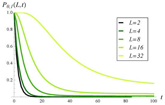
Figure 5.
Probability that the size of the queue is under L in interval , for different values of L.
At the end of this section, we will see a different picture in the case of a negative correlation.
In Figure 6, the distributions (densities) of the time to reach the critical level L are shown for a few values of L. The average values for these distributions are 2.4, 3.4, 8.9, 29.7, and 107.5 for , , , , and , respectively. As could be expected, for small L, the probability mass in Figure 6 is strongly concentrated around 0, and the average value is very small. However, even for the full buffer (), the average time to hit, 107.5, is considerably small. This again is a result of the very strong, positive autocorrelation of the arrival process.
Figure 6.
Density function of the time to cross level L, for different values of L.
Now, we will check how the level-crossing characteristics depend on the service speed and parameterization of AQM (i.e., ).
To achieve this, we will apply a scaled version of the transmission time, , where is a scaling parameter while is a random variable distributed according to (72). Naturally, we have . Therefore, scaling a from 0 to 1.5 will automatically scale the average transmission time from 0 to 1.5.
Furthermore, we will use a parameter-dependent AQM mechanism in the form
where is a parameter, whereas function is defined in (71). The larger the value of C, the more aggressive the active management is—it deletes more packets and for lower queue sizes.
In Figure 7, the probability of not hitting level 25 by the time 100 s is depicted as a function of and C. As can be expected, the probability increases with C and decreases with . Furthermore, the dependence on is gradual, while the dependence on C has a sharp step. Indeed, for a sufficiently aggressive deletion policy, there is a high probability of keeping the queue low.
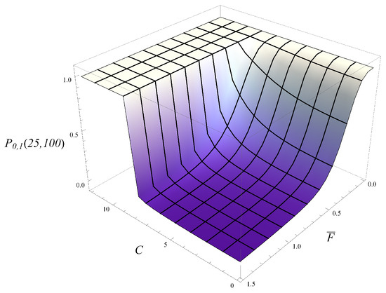
Figure 7.
Probability that the size of the queue is below in interval depending on the average transmission time, , and the active management parameter, C.
In Figure 8, the average time to flush the buffer is shown as a function of and C. As anticipated, this average time decreases with C and increases with . No sharp steps like the one seen in Figure 7 are present. This is easy to explain. Namely, when obtaining Figure 8, it was assumed that the buffer was initially full, so every packet inside had already passed the AQM mechanisms. Of course, this mechanism will still be applied to newly arriving packets, but when the transmission process is fast, the average time to flush is more affected by the packets already deposited in the buffer.
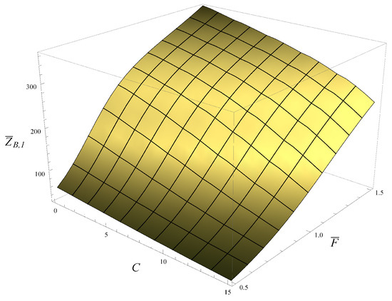
Figure 8.
Average time needed to flush the buffer, depending on the average transmission time, , and the active management parameter, C.
4.1. Application Scenarios—Sample Solutions
Consider now a wireless sensor node utilizing the N-policy, as described in Section 1, where the output radio interface is activated when the size of the queue reaches 30 packets.
From formula (57), we can directly obtain the average buffer flush time for given values of and C. For instance, if and , then the average buffer flush time is . The energy consumption of the output radio interface in one flush cycle is obviously proportional to this time. Therefore, we can easily compute this energy if we know the energy consumption of an active radio per second.
Next, we may ask how long the idle period is, i.e., the period when the size of the queue grows from 0 to 30. This can be computed from formula (37) using , because transmission is suspended during the idle period. For , the duration of the idle period is .
Then, we can reverse the first problem mentioned and ask: what is the minimum transmission rate during the active period that guarantees the average buffer flush time (active period) to be no more than 100 s?
The solution to such a problem with can be obtained by taking a vertical slice of Figure 8 for . This slice is depicted in Figure 9. As is visible in Figure 9, the maximum transmission time that provides is , which translates to a minimum transmission rate of 1.65 packets/s.
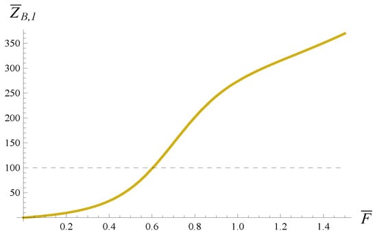
Figure 9.
Average time needed to flush the buffer depending on the average packet transmission time. .
In the previous problem, we optimized only the transmission rate to achieve a specific goal. Obviously, we can simultaneously optimize C as well.
Namely, we can ask: which combinations of parameters provide an average flush time of no more than 100 s?
To solve such a problem, we horizontally cut Figure 8 at the level of 100.
The result is depicted in Figure 10. The grey area in Figure 10 represents the set of all combinations of parameters that provide an average buffer flush time below 100 s.
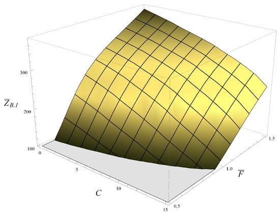
Figure 10.
Combinations of parameters C and which provide an average time required to flush the buffer below 100 s (grey area).
4.2. Negative Autocorrelation
All of the previous calculations were carried out for the positively correlated traffic, parameterized in (67)–(70). In the remaining calculations, we will use the following traffic parameters:
For these parameters, the arrival rate is 1 again, the mean batch size is 4.66 again, but the 1-lag autcorrelation is . Therefore, we now have a strong negative autocorrelation.
All the remaining parameters of the system are unaltered. Therefore, comparing the new results with the previous ones, we will see the raw effect of autocorrelation.
In Figure 11, the probability that the size of the queue is under L until t is depicted for a few values of L. This figure is to be compared with Figure 5 procured for the positive autocorrelation.
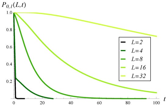
Figure 11.
Probability that the size of the queue is under L in interval for different values of L. Negative autocorrelation.
First of all, we see significant influence from autocorrelation; the figures differ substantially from each other. For high and moderate critical levels L, the probability of not hitting L decreases much slower in Figure 11 than in Figure 5. However, for a low value of L, this probability decreases much faster in Figure 11 than in Figure 5.
In Figure 12, distributions (densities) of the time to hit L are shown for a few values of L. The average values for distributions shown in Figure 12 are 0.3, 2.8, 13.1, 40.0, and 247.1 for , , , , and respectively.
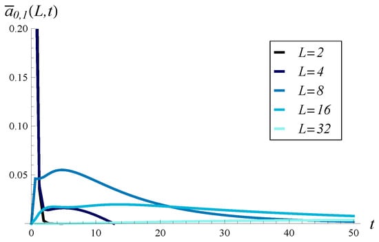
Figure 12.
Density function of the time to cross level L for different values of L. Negative autocorrelation.
For small L, the probability mass in Figure 12 is more concentrated around 0 than in Figure 6, while for high L, a reverse effect is seen. We see this effect also when comparing the average hitting times. We have average hitting times of 0.3 vs. 2.4 (); 2.8 vs. 3.4 (); 13.1 vs. 8.9 (); 40.0 vs. 29.7 (); and 247.1 vs. 107.5 (). In each pair, the first value is calculated for the negative autocorrelation, while the second is calculated for the positive autocorrelation.
These results clearly indicate that neither positive nor negative autocorrelation result in all the level-crossing characteristics being uniformly worse. In some cases, the positive autocorrelation produces worse results (i.e., higher hitting probabilities, shorter hitting times), while in other cases, the negative autocorrelation produces worse results. This observation is rather surprising.
So far, we have seen the effect of autocorrelation for different values of the critical level L.
In Figure 13, we can see the effect of autocorrelation for different values of t. Namely, in this figure, the probability that the size of the queue is kept below 4 in interval is depicted for both positive and negative autocorrelation.
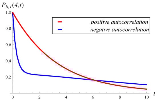
Figure 13.
Probability that the buffer occupancy is under 4 in for positive and negative autocorrelation.
We see again that neither positive nor negative autocorrelation prevails. For a small t, positive autocorrelation induces a higher no-hit probability, while for a large t, the opposite is true.
In the next two figures, the dependence of the level-crossing characteristics on the transmission speed and the active management parameterization is depicted for the negative autocorrelation.
In Figure 14, the probability that the size of the queue is kept below level 25 until is shown as a function of and C. This figure is to be compared with Figure 7, which was obtained for the positive autocorrelation. We see that the no-hit probability decreases more slowly with when the autocorrelation is negative. On the flip side, the no-hit probability increases more quickly with C when the autocorrelation is negative.
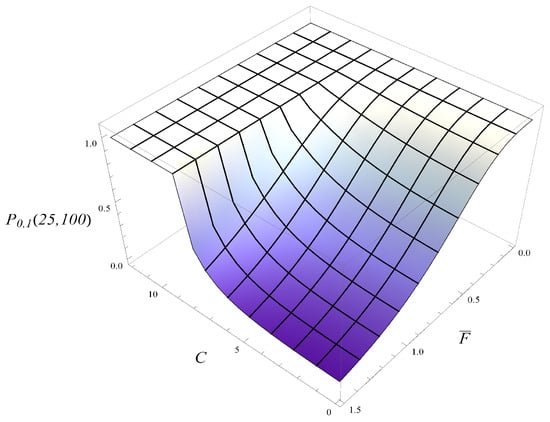
Figure 14.
Probability that the size of the queue is under 25 in interval depending on the average transmission time, , and the active management parameter, C. Negative autocorrelation.
Finally, the average buffer flush time as a function of and C is depicted in Figure 15, which can be compared with Figure 8, obtained for the positive autocorrelation.
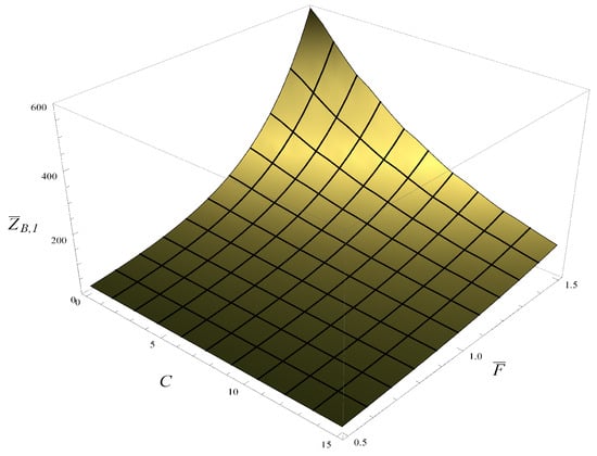
Figure 15.
Average time needed to flush the buffer, depending on the average transmission time, , and the active management parameter, C. Negative autocorrelation.
5. Conclusions
We derived several level-crossing metrics for a buffer with an AQM mechanism. These metrics include the probability of keeping the queue size below a predefined level L, the distribution of the time needed to hit level L, the buffer overflow probability, the average time until overflow, the distribution of the buffer flush time, and its mean value.
Among other things, these metrics characterize the performance of the AQM mechanism by assessing how effectively it prevents the queue of packets from growing too long and how it assists in flushing the buffer quickly, if necessary.
A general modeling framework was used in derivations, with a general service time distribution, general rejection function, and a powerful model of the arrival process.
Through numerical examples, we explored the influence of various model parameters on different level-crossing metrics and demonstrated the utility of the obtained formulas.
A special emphasis was placed on the investigation of traffic autocorrelation impact on the level-crossing characteristics. It was shown that autocorrelation significantly affects these characteristics, with neither positive nor negative autocorrelation uniformly worsening all metrics. In some cases, positive autocorrelation results in higher hitting probabilities and shorter hitting times, while in others, negative autocorrelation produces worse results. This is a rather unexpected finding.
The obtained results are especially useful in the analysis of the energy efficiency of a wireless sensor node equipped with the N-policy and AQM. Under such a policy, the output radio is switched off until the queue of packets reaches a critical size.
As demonstrated in Section 4.1, the obtained formulas allow for computing the average duration of the idle period and the average duration of the active period. Combining the two, we can obtain the long-run fraction of time when the output ratio is on. Therefore, we can compute its average energy consumption over time.
There are other possible directions for future work on the performance of a wireless sensor node with the N-policy and AQM. The active and idle periods of this mechanism are not the only two characteristics of interest. Equally important are, for instance, the queuing delay and the packet loss ratio. These characteristics have not yet been found for a buffer with the N-policy and AQM.
Other future work could be devoted to level-crossing characteristics for an AQM of a different type. Here, we consider the popular type of AQM, which rejects packets based on buffer occupancy. However, this is not the only possible type. In other AQMs, packets can be rejected based on queuing latency, virtual queues, empty buffer events, and other factors. Moreover, the rejection probability in some AQMs is updated at regular time intervals rather than upon new packet arrivals.
Funding
This research received no external funding.
Data Availability Statement
Data is contained within the article.
Conflicts of Interest
The author declare no conflicts of interest.
References
- Internet Engineering Task Force. Request for Comments 7567: ETF Recommendations Regarding Active Queue Management; Baker, F., Fairhurst, G., Eds.; Internet Engineering Task Force: Fremont, CA, USA, 2015. [Google Scholar]
- Internet Engineering Task Force. Request for Comments 7928: Characterization Guidelines for Active Queue Management (AQM); Kuhn, N., Natarajan, P., Khademi, N., Eds.; Internet Engineering Task Force: Fremont, CA, USA, 2016. [Google Scholar]
- Ghaffari, A. Congestion control mechanisms in Wireless Sensor Networks: A survey. J. Netw. Comput. Appl. 2015, 52, 101–115. [Google Scholar] [CrossRef]
- Asonye, E.A.; Musa, S.M. Analysis of Personal Area Networks for ZigBee Environment Using Random Early Detection-Active Queue Management Model. In Proceedings of the International Conference on Industrial Engineering and Operations Management, Toronto, ON, Canada, 23–25 October 2019; pp. 1441–1455. [Google Scholar]
- Kumar, H.; Kumar, S.M.D.; Nagarjun, E. Congestion Estimation and Mitigation Using Fuzzy System in Wireless Sensor Network. Lect. Notes Netw. Syst. 2022, 329, 655–667. [Google Scholar]
- Paul, A.K.; Kawakami, H.; Tachibana, A.; Hasegawa, T. An AQM based congestion control for eNB RLC in 4G/LTE network. In Proceedings of the IEEE Canadian Conference on Electrical and Computer Engineering (CCECE), Vancouver, BC, Canada, 15–18 May 2016; pp. 1–5. [Google Scholar]
- Jafri, S.T.A.; Ahmed, I.; Ali, S. Queue-Buffer Optimization Based on Aggressive Random Early Detection in Massive NB-IoT MANET for 5G Applications. Electronics 2022, 11, 2955. [Google Scholar] [CrossRef]
- Kumar, K.; Ramya, I.; Masillamani, M. Queue management in mobile adhoc networks (MANETS). In Proceedings of the IEEE/ACM International Conference on Green Computing and Communications, Hangzhou, China, 17–21 December 2010; pp. 943–946. [Google Scholar]
- Mahajan, M.; Singh, T.P. The Modified Gaussian Function based RED (MGF-RED) Algorithm for Congestion Avoidance in Mobile Ad Hoc Networks. Int. J. Comput. Appl. 2014, 91, 39–44. [Google Scholar] [CrossRef]
- Bie, Y.; Li, Z.; Hu, Z.; Chen, J. Queue Management Algorithm for Satellite Networks Based on Traffic Prediction. IEEE Access 2022, 10, 54313–54324. [Google Scholar] [CrossRef]
- Hou, K.; Yang, J.; Liu, F.; Zhang, C. An Active Queue Management Algorithm to Guarantee the QoS of LEO Satellite Network. In Proceedings of the International Symposium on Computer Technology and Information Science (ISCTIS), Chengdu, China, 16–18 June 2023. [Google Scholar]
- Floyd, S.; Jacobson, V. Random early detection gateways for congestion avoidance. IEEE/ACM Trans. Netw. 1993, 1, 397–413. [Google Scholar] [CrossRef]
- Zhou, K.; Yeung, K.L.; Li, V. Nonlinear RED: Asimple yet efficient active queue management scheme. Comput. Netw. 2006, 50, 3784–3794. [Google Scholar] [CrossRef]
- Zhang, S.; Sa, J.; Liu, J.; Wu, S. An improved RED algorithm with sinusoidal packet-marking probability and dynamic weight. In Proceedings of the International Conference on Electric Information and Control Engineering, Wuhan, China, 15–17 April 2011; pp. 1160–1163. [Google Scholar]
- Augustyn, D.R.; Domanski, A.; Domanska, J. A choice of optimal packet dropping function for active queue management. Commun. Comput. Inf. Sci. 2010, 79, 199–206. [Google Scholar]
- Domanska, J.; Augustyn, D.; Domanski, A. The choice of optimal 3-rd order polynomial packet dropping function for NLRED in the presence of self-similar traffic. Bull. Pol. Acad. Sci. Tech. Sci. 2012, 60, 779–786. [Google Scholar] [CrossRef]
- Hussein, A.-J. An Exponential Active Queue Management Method Based on Random Early Detection. J. Comput. Netw. Commun. 2020, 2020, 8090468. [Google Scholar]
- Gimenez, A.; Murcia, M.A.; Amigo, J.M.; Martínez-Bonastre, O.; Valero, J. New RED-Type TCP-AQM Algorithms Based on Beta Distribution Drop Functions. Appl. Sci. 2022, 12, 11176. [Google Scholar] [CrossRef]
- Hassan, S.O.; Rufai, A.; Ajaegbu, C.; Ayankoya, F.Y. DL-RED: A RED-based algorithm for routers. Int. J. Comput. Appl. Technol. 2022, 70, 244–253. [Google Scholar] [CrossRef]
- Hassan, S.O.; Nwaocha, V.O.; Rufai, A.U.; Odule, T.J.; Enem, T.A.; Ogundele, L.A.; Usman, S.A. Random early detection-quadratic linear: An enhanced active queue management algorithm. Bull. Electr. Eng. Inform. 2022, 11, 2262–2272. [Google Scholar] [CrossRef]
- Feng, C.; Huang, L.; Xu, C.; Chang, Y. Congestion Control Scheme Performance Analysis Based on Nonlinear RED. IEEE Syst. J. 2017, 11, 2247–2254. [Google Scholar] [CrossRef]
- Hassan, S.O.; Rufai, A. Modified dropping-random early detection (MD-RED): A modified algorithm for controlling network congestion. Int. J. Inf. Technol. 2023, 15, 1499–1508. [Google Scholar] [CrossRef]
- Hassan, S.O.; Rufai, A.U.; Nwaocha, V.O.; Ogunlere, S.O.; Adegbenjo, A.A.; Agbaje, M.O.; Enem, T.A. Quadratic exponential random early detection: A new enhanced random early detection-oriented congestion control algorithm for routers. Int. J. Electr. Comput. Eng. 2023, 13, 669–679. [Google Scholar] [CrossRef]
- Nichols, K.; Jacobson, V. Controlling Queue Delay. Queue 2012, 55, 42–50. [Google Scholar]
- Kahe, G.; Jahangir, A.H. A self-tuning controller for queuing delay regulation in TCP/AQM networks. Telecommun. Syst. 2019, 71, 215–229. [Google Scholar] [CrossRef]
- Wang, H. Trade-off queuing delay and link utilization for solving bufferbloaTrade-off queuing delay and link utilization for solving bufferbloat. ICT Express 2020, 6, 269–272. [Google Scholar] [CrossRef]
- Hotchi, R.; Chibana, H.; Iwai, T.; Kubo, R. Active queue management supporting TCP flows using disturbance observer and Smith predictor. IEEE Access 2020, 8, 173401–173413. [Google Scholar] [CrossRef]
- Wang, C.; Chen, X.; Cao, J.; Qiu, J.; Liu, Y.; Luo, Y. Neural Network-Based Distributed Adaptive Pre-Assigned Finite-Time Consensus of Multiple TCP/AQM Networks. IEEE Trans. Circuits Syst. 2021, 68, 387–395. [Google Scholar] [CrossRef]
- Shen, J.; Jing, Y.; Ren, T. Adaptive finite time congestion tracking control for TCP/AQM system with input saturation. Int. J. Syst. Sci. 2022, 53, 253–264. [Google Scholar] [CrossRef]
- Barczyk, M.; Chydzinski, A. AQM based on the queue length: A real-network study. PLoS ONE 2022, 17, e0263407. [Google Scholar] [CrossRef] [PubMed]
- Jiang, F.C.; Huang, D.C.; Wang, K.H. Design approaches for optimizing power consumption of sensor node with N-policy M/G/1 queuing model. In Proceedings of the International Conference on Queueing Theory and Network Applications, ACM, Singapore, 29–31 July 2009; pp. 1–8. [Google Scholar]
- Maheswar, R.; Jayaparvathy, R. Power control algorithm for wireless sensor networks using N-policy M/M/1 queueing model. Power 2010, 2, 2378–2382. [Google Scholar]
- Jiang, F.C.; Huang, D.C.; Yang, C.T.; Leu, F.Y. Lifetime elongation for wireless sensor network using queue-based approaches. J. Supercomput. 2012, 59, 1312–1335. [Google Scholar] [CrossRef]
- Ma, Z.; Yu, X.; Guo, S.; Zhang, Y. Analysis of wireless sensor networks with sleep mode and threshold activation. Wirel. Netw. 2021, 27, 1431–1443. [Google Scholar] [CrossRef]
- Kempa, W.M.; Kurzyk, D. On Transient Queue-Size Distribution in a Model of WSN Node with Threshold-Type Power-Saving Algorithm. Sensors 2022, 22, 9285. [Google Scholar] [CrossRef]
- Arumugam, S.K.; Mohammed, A.S.; Nagarajan, K.; Ramasubramanian, K.; Goyal, S.B.; Verma, C.; Mihaltan, T.C.; Safirescu, C.O. A Novel Energy Efficient Threshold Based Algorithm for Wireless Body Sensor Network. Energies 2022, 15, 6095. [Google Scholar] [CrossRef]
- Chaudhry, M.L.; Zhao, Y.Q. First-passage time and busy period distributions of discrete-time Markovian queues: Geom(n)/Geom(n)/1/N. Queueing Syst. 1994, 18, 5–26. [Google Scholar] [CrossRef]
- Ross, S.M.; Seshadri, S. Hitting time in an M/G/1 queue. J. Appl. Probababilty 1999, 36, 934–940. [Google Scholar] [CrossRef]
- Asmussen, S.; Jobmann, M.; Schwefel, H.P. Exact buffer overflow calculations for queues via Martingales. Queueing Syst. 2002, 42, 63–90. [Google Scholar] [CrossRef]
- Chydzinski, A. Time to reach buffer capacity in a BMAP queue. Stoch. Model. 2007, 23, 195–209. [Google Scholar] [CrossRef]
- Kempa, W.M. On time-to-buffer overflow distribution in a single-machine discrete-time system with finite capacity. Math. Model. Anal. 2020, 25, 289–302. [Google Scholar] [CrossRef]
- Kempa, W.M.; Marjasz, R. Distribution of the time to buffer overflow in the M/G/1/N-type queueing model with batch arrivals and multiple vacation policy. J. Oper. Res. Soc. 2020, 71, 447–455. [Google Scholar] [CrossRef]
- Kobielnik, M.; Kempa, W. On the Time to Buffer Overflow in a Queueing Model with a General Independent Input Stream and Power-Saving Mechanism Based on Working Vacations. Sensors 2021, 21, 5507. [Google Scholar] [CrossRef] [PubMed]
- Bonald, T.; May, M.; Bolot, J.-C. Analytic evaluation of RED performance. In Proceedings of the IEEE INFOCOM 2000 Conference on Computer Communications, 19th Annual Joint Conference of the IEEE Computer and Communications Societies, Hong Kong, China, 7–11 March 2000; pp. 1415–1424. [Google Scholar]
- Hao, W.; Wei, Y. An Extended GIX/M/1/N Queueing Model for Evaluating the Performance of AQM Algorithms with Aggregate Traffic. Lect. Notes Comput. Sci. 2005, 3619, 395–414. [Google Scholar]
- Kempa, W.M. A direct approach to transient queue-size distribution in a finite-buffer queue with AQM. Appl. Math. Inf. Sci. 2013, 7, 909–915. [Google Scholar] [CrossRef]
- Tikhonenko, O.; Kempa, W.M. Performance evaluation of an M/G/N-type queue with bounded capacity and packet dropping. Appl. Math. Comput. Sci. 2016, 26, 841–854. [Google Scholar] [CrossRef]
- Tikhonenko, O.; Kempa, W.M. Erlang service system with limited memory space under control of AQM mechanizm. Commun. Comput. Inf. Sci. 2017, 718, 366–379. [Google Scholar]
- Chydzinski, A. Non-Stationary Characteristics of AQM Based on the Queue Length. Sensors 2023, 23, 485. [Google Scholar] [CrossRef]
- Chydzinski, A. Loss Process at an AQM Buffer. J. Sens. Actuator Netw. 2023, 12, 55. [Google Scholar] [CrossRef]
- Chydzinski, A. On the Transient Queue with the Dropping Function. Entropy 2020, 22, 825. [Google Scholar] [CrossRef] [PubMed]
- Lel, W.; Taqqu, M.; Willinger, W.; Wilson, D. On the self-similar nature of ethernet traffic (extended version). IEEE/ACM Trans. Netw. 1994, 2, 1–15. [Google Scholar]
- Lucantoni, D.M. New results on the single server queue with a batch Markovian arrival process. Commun. Stat. Stoch. Model. 1991, 7, 1–46. [Google Scholar] [CrossRef]
- Salvador, P.; Pacheco, A.; Valadas, R. Modeling IP traffic: Joint characterization of packet arrivals and packet sizes using BMAPs. Comput. Netw. 2004, 44, 335–352. [Google Scholar] [CrossRef]
- Garetto, M.; Towsley, D. An efficient technique to analyze the impact of bursty TCP traffic in wide-area networks. Perform. Eval. 2008, 65, 181–202. [Google Scholar] [CrossRef]
- Dudin, A.N.; Klimenok, V.I.; Vishnevsky, V.M. The Theory of Queuing Systems with Correlated Flows; Springer: Cham, Switzerland, 2020. [Google Scholar]
- Chydzinski, A. Queue Size in a BMAP Queue with Finite Buffer. Lect. Notes Comput. Sci. 2006, 4003, 200–210. [Google Scholar]
- Schiff, J.L. The Laplace Transform: Theory and Applications; Springer: New York, NY, USA, 1999. [Google Scholar]
- Zakian, V. Numerical inversion of Laplace transform. Electron. Lett. 1969, 5, 120–121. [Google Scholar] [CrossRef]
- Chydzinski, A.; Mrozowski, P. Queues with dropping functions and general arrival processes. PLoS ONE 2016, 11, e0150702. [Google Scholar] [CrossRef]
Disclaimer/Publisher’s Note: The statements, opinions and data contained in all publications are solely those of the individual author(s) and contributor(s) and not of MDPI and/or the editor(s). MDPI and/or the editor(s) disclaim responsibility for any injury to people or property resulting from any ideas, methods, instructions or products referred to in the content. |
© 2024 by the author. Licensee MDPI, Basel, Switzerland. This article is an open access article distributed under the terms and conditions of the Creative Commons Attribution (CC BY) license (https://creativecommons.org/licenses/by/4.0/).