Optimal Signal Wavelengths for Underwater Optical Wireless Communication under Sunlight in Stratified Waters

Abstract

Underwater optical wireless communication (UOWC) is a field of research that has gained popularity with the development of unmanned underwater vehicle (UUV) technologies. Its utilization is crucial in offshore industries engaging in sustainable alternatives for food production and energy security. Although UOWC can meet the high data rate and low latency requirements of underwater video transmission for UUV operations, the links that enable such communication are affected by the inhomogeneous light attenuation and the presence of sunlight. Here, we present how the underwater spectral distribution of the light field can be modeled along the depths of eight stratified oceanic water types. We considered other established models, such as SPCTRL2, Haltrin’s single parameter model for inherent optical properties, and a model for the estimation of the depth distribution of chlorophyll-a, and present insights based on transmission wavelength for the maximum signal-to-noise ratio (SNR) under different optical link parameter combinations such as beam divergence and transmit power under “daytime” and “nighttime” conditions. The results seem to challenge the common notion that the blue-green spectrum is the most suitable for underwater optical communication. We highlight a unique relationship between the transmission wavelength for the optimal SNR and the link parameters and distance, which varies with depth depending on the type of oceanic water stratification. Our analyses further highlighted potential implications for solar discriminatory approaches and strategies for routing in cooperative optical wireless networks in the photic region.

1. Introduction

With the growing demand for food and energy resources and exacerbating climate conditions, many authorities across the globe are exploring ways to venture into the oceans for sustainable aquacultural and industrial alternatives. Collectively termed as the “Blue Economy”, offshore ventures such as aquaculture farms, carbon-capture facilities, and the provision of renewable energy (wind, wave, and solar) are some examples of ocean-based economic activities that are expected to reach 3 trillion USD per annum by the year 2030 [1]. Other supplementary activities, such as maritime safety and surveillance, and maritime and coastal tourism, are expected to develop around these ventures, involving resources from the fields of environmental science, oceanography, marine robotics, national security, transportation, and even consumer electronics [1]. Partners of these blue economy activities have recognized the importance of automating offshore underwater tasks, such as monitoring fish health and biofouling inside aquaculture enclosures, conducting seabed surveys, or inspecting and repairing underwater pipelines and cables, using remotely operated or autonomous underwater vehicles (ROVs or AUVs) that would otherwise require divers, offering better efficiency, accuracy, and safety for a better economic outcome [2,3,4,5,6,7,8]. These operations may require coordination between networks of remote vehicles and other submerged devices. For example, this may consist of a series of miniature biomimetic robots or a swarm of AUVs coordinating with solar-powered buoys and seabed-moored sensors to accomplish a mission [9,10,11,12]. Tethers are the most common approach of communication between human operators and these underwater vehicles, termed collectively as unmanned underwater vehicles (UUVs). However, tethers limit UUV maneuverability and range due to drag, tension, and finite length, respectively, and are prone to entanglement and breakage, thus limiting the potential for swarmed operations [4,8,13,14,15,16]. Tethers are also subject to biofouling during long-term deployments.

The alternative is to establish wireless forms of communication using acoustic, radiofrequency, optical, or electromagnetic links. Acoustic underwater communication, the most developed form, dates back to the late 1980s. Acoustic transmissions of image and control information over vast distances have been demonstrated since the late 1980s [17,18]. However, they operate in the audible-ultrasound range (around 20 kHz), resulting in low bandwidths and data rates in the tens of kbps [19,20]. Furthermore, although sound spreads outward as a mechanical wave with low directionality, it introduces challenges like reflections, multipaths, and channel saturation. The slow speed of sound in water of about 1500 m s⁻¹ is influenced by temperature, pressure, and salinity variations in the vertical channels (where link direction is vertical), and are further susceptible to ocean currents and Doppler effects causing delay spread and intersymbol interference (ISI) [21,22]. Acoustic modems, though robust, are also cumbersome and costly, thus prompting the development of alternative solutions for wireless multimedia transmission for mobile underwater systems. Radiofrequencies (RF) may be more favorable candidates for underwater communication because these can achieve higher data rates, bandwidths, throughputs, and lower latencies. The use of RF, however, is limited to extremely low-frequency ranges due to severe spectrum attenuation, and this requires large antennas and transmission power, posing challenges for compact UUVs [19,23,24]. Shallow-water strategies such as propagating the signal over the water–air barrier may reduce attenuation [25], but this might not be suitable for all applications. Magnetic induction (MI) for underwater communication, on the other hand, a novel research area, is based on inducing signals between coils of wire. The technology is relatively new, with a limited transmission range and challenges with the alignment of coils, complicating mobile scenarios [26]. Recent work explores sound-driven triboelectric nanogenerators (TENGs) as an alternative [27]. While promising, TENG’s fundamental frequency currently limits data rates, requiring extensive research before high-bandwidth information transmission becomes feasible.

In contrast, underwater optical wireless communication (UOWC) employs light frequencies within the visible range of the electromagnetic spectrum (EM), taking advantage of wavelengths that show the least attenuation. Such communication enables the transmission of >1 Gbps over few hundred meters in point-to-point (P2P) configurations. For example, Li et al. and Wu et al. have showcased data transmission rates of 16.4 Gbps (488 nm, up to 10 m range) and 12.4 Gbps (450 nm, up to 1.7 m range), respectively, using lasers [28,29]. They have also achieved a 205 Mbps connection over a 10 m distance using blue light-emitting diodes (460 nm LED array with 70 W total output) [30].

UOWC faces challenges such as directionality, where light obstructed by objects like fish or debris may cause signal loss. The inclusion of multipath propagations could address this, but with limitations in shallow water. In shallow water, the length of the alternative signal path may exceed transmission distances, leading to greater attenuation and also absorption of reflected multipaths by the seafloor [19,24]. In addition to this, environmental conditions such as ambient light, scattering from suspended particles, and refraction with varying refractive indices along the propagation pathway deteriorate signal quality. Nevertheless, these drawbacks may be overcome if the system’s adaptability is improved, given that UOWC’s potential is underscored by the channel’s high capacity, low latency, and low cost per bit compared to other wireless alternatives. For example, off-the-shelf components such as lasers, LEDs, and photodiodes (PD) can be used to build high-frequency emitters and receivers and thus employ modulation and diversity schemes that enhance bandwidth and range, which is an advantage over acoustic or RF systems that require costly, complex transducers [31]. Furthermore, even though optical link ranges are of moderate length compared to acoustic options, this could be beneficial toward the cellularization of networks with better security advantages and improved sharing of bandwidth, similar to wi-fi, while multihopping could be a sound solution if long distance communication is needed [32]. This way, by adopting strategies like those used in existing terrestrial mobile wireless networks, UOWC networks could be established as both localized and widespread (cooperative) connections between UUVs and other static or mobile devices, as shown in Figure 1.

The spectra favorable for UOWC span a bandwidth that is within the solar spectrum. Sunlight may therefore affect link quality. In addition to this, UOWC SNR studies often ignore that ocean bodies are inhomogeneous. The effects of sunlight and medium inhomogeneity on transmission wavelengths and beam characteristics are underexplored. Therefore, to address this research gap, we have

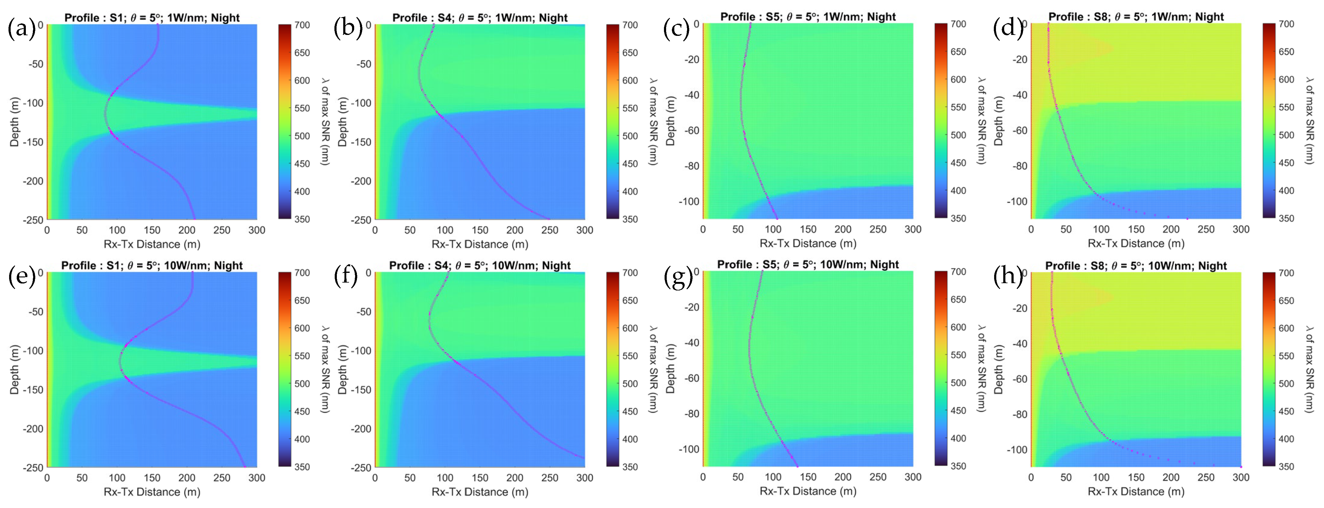
• Investigated the effect of attenuation on the end-to-end diffused line-of-sight and point-to-point line-of-sight UOWC systems under eight realistic ocean stratification scenarios in order of increasing turbidity, under a “night condition”.
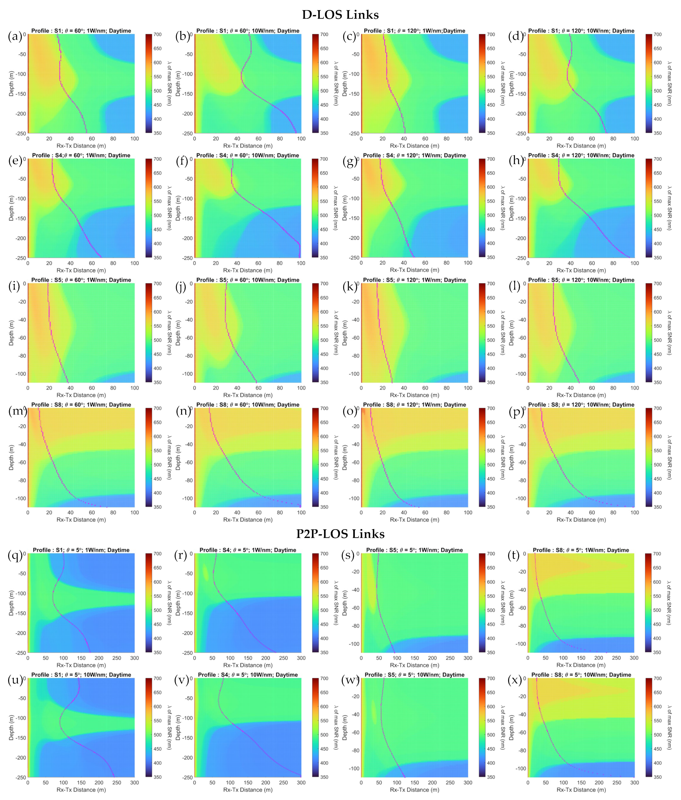
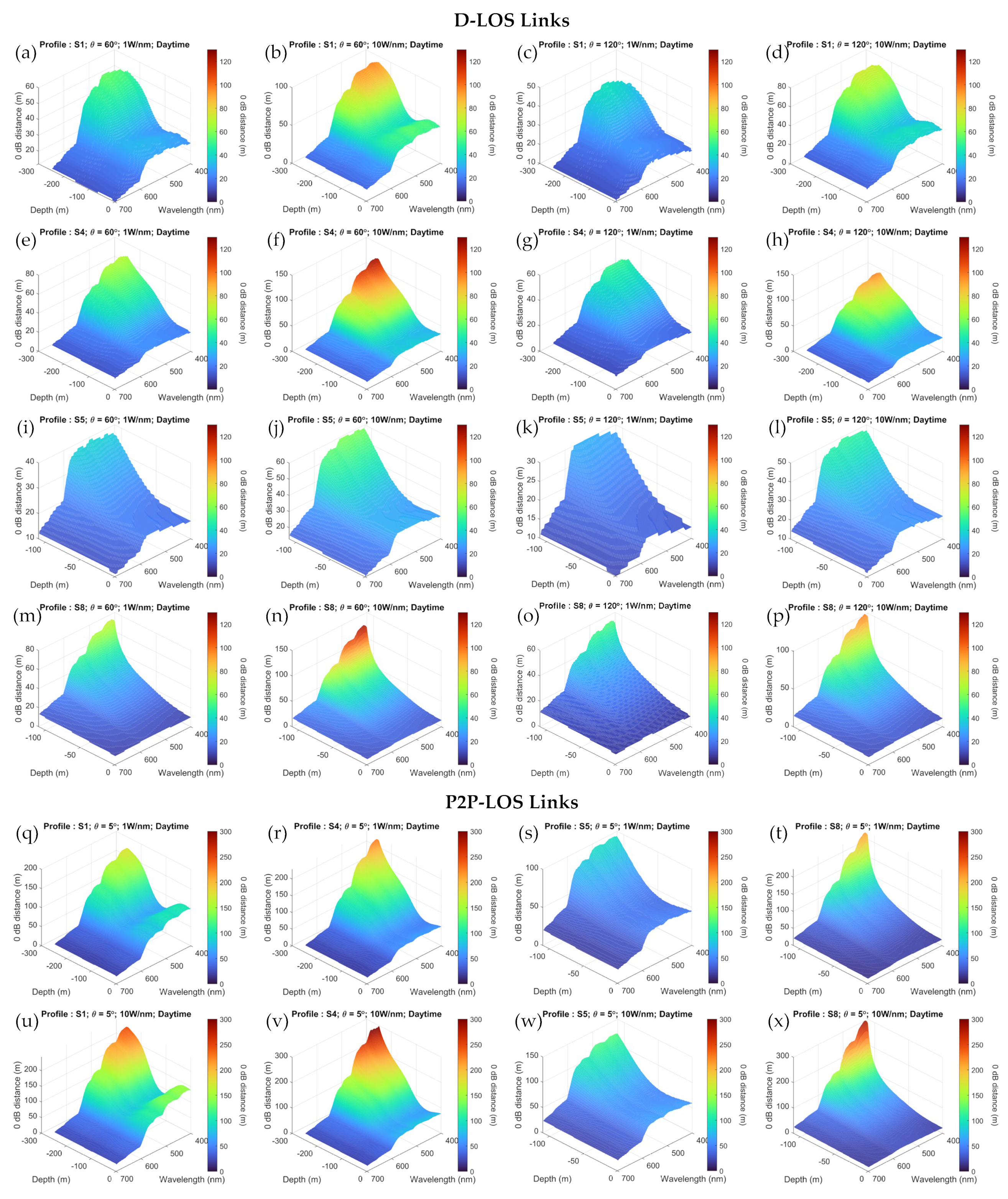
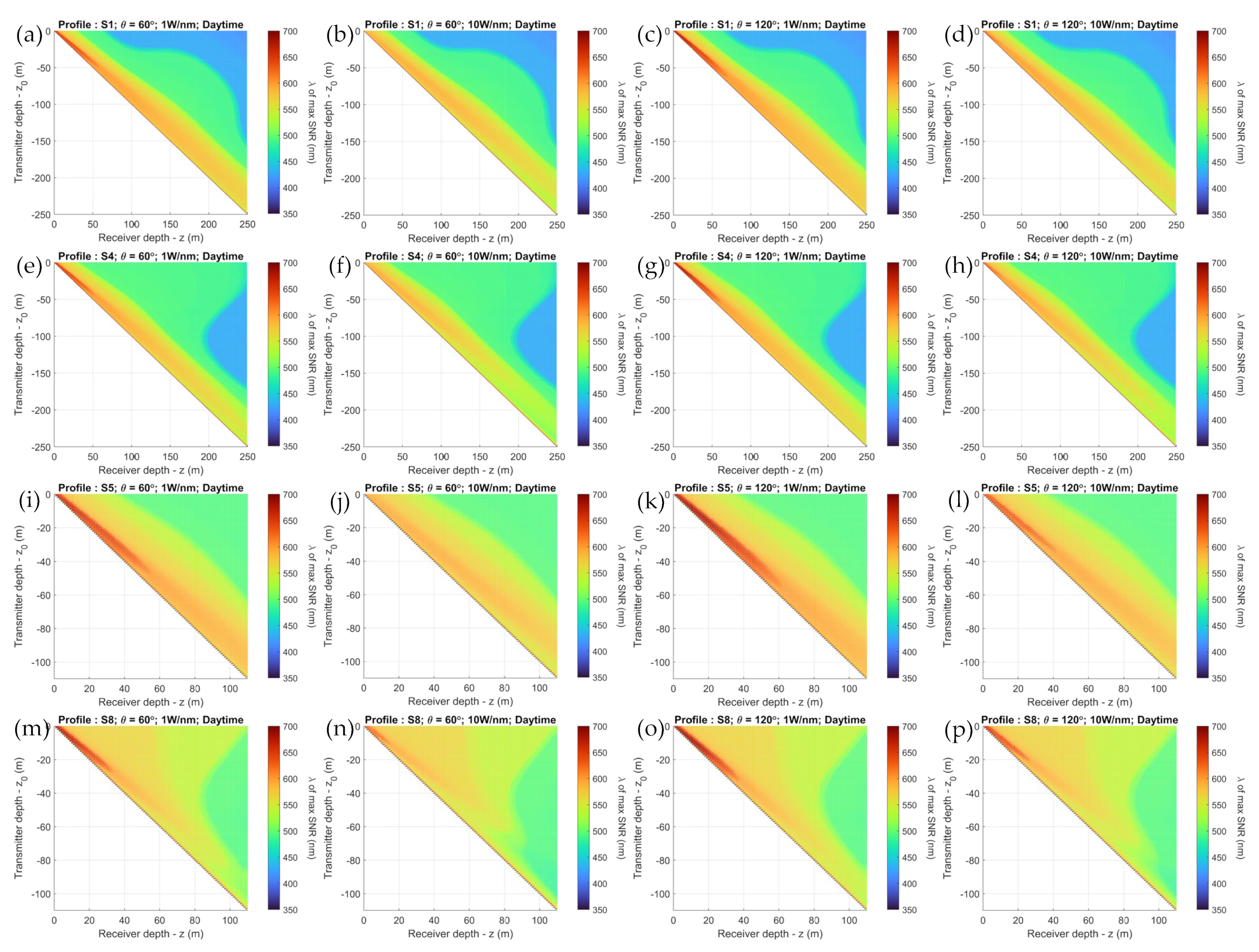
• Investigated the combined effect of signal attenuation and ambient solar radiation on end-to-end diffused line-of-sight and point-to-point line-of-sight UOWC systems under the eight stratification scenarios. This was evaluated for horizontal links and downlinks (transmitter is vertically above the receiver, with the receiver directly facing up in direct view of sunlight) by varying depth and distance.
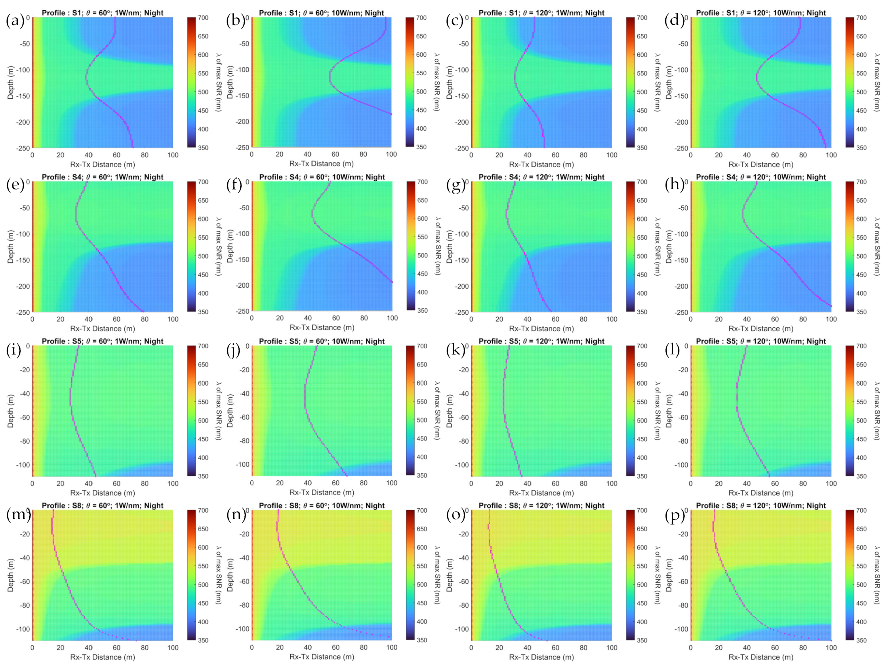
• Shared novel insights on the wavelength preferences for the signal (400–700 nm) for the optimum optical signal-to-noise ratio (O-SNR) under the conditions described above, that seems to be connected to the transmitter and receiver parameters such as transmit power, beam divergence, and the receiver (photodetector) wavelength responsivity curve. The results have been shown with trends discussed for four selected profiles for brevity, in order of increasing turbidity.
• Demonstrated the variability of the maximum achievable link distance with depth based on the O-SNR (0 dB distance) correlated to the signal wavelength that achieves it.
• Shared insights on how these findings may be used to establish cooperative UOWC links for the optimal SNR, based on water profile, depth relative to the deep chlorophyll maximum, link orientation, and distance between the nodes. These findings may be useful for establishing UOWC within individual sites, such as aquaculture farms, or renewable energy sites if the site-specific water quality parameters are known and where the region of the UUV mission or connectivity of the UOWC network would span depths of the euphotic and disphotic zones.
• Provided re-evaluated coefficients to ensure the attenuation model detailed in Johnson et al. [33] is consistent with Uitz et al. [34].

2. Preliminaries

A generic UOWC involves a transmitter generating photons that traverse through water and convert into electrical signals at the receiver. The data generated by a UUV are modulated onto an optical carrier of a specific wavelength, amplified, beam-shaped, and transmitted. At the receiver, the photons from the transmitted light are collected by lenses into a photodetector that converts them into electrical signals, which are then amplified, noise-filtered, and demodulated to recover the data (Figure 2) [19].

Photon transmission underwater depends on the inherent and apparent optical properties (IOP and AOP) of water [20]. While IOPs relate to the absorption and scattering of light by solutes and particulates, AOPs relate to physical parameters defining the optical beam’s structure. AOPs are tied to engineering choices like beam divergence angle and those defined by medium composition, such as the reflectance. The combined effects of absorption and scattering give rise to signal attenuation in which a portion of signal energy is either converted to another energy form (chemical or heat) or is redirected away from the intended path. The overall wavelength-dependent signal attenuation c(λ), as expressed in (1), is the sum of absorption a(λ) and scattering b(λ) coefficients at a vacuum wavelength of light λ in nm.

$$c\left(\lambda \right)=a\left(\lambda \right)+b\left(\lambda \right)$$

(1)

The nominal values for $c$: 0.056, 0.15, 0.305, and 2.17 m⁻¹ are used for modeling pure seawater, clear ocean water, coastal ocean water, and turbid water in harbors, respectively [19,35]. The classification by Jerlov [36], which has been widely used in parametric simulations of UOWC, identifies ten types of seawater. Types I, IA, IB, II, and III are clear-oceanic waters, and types 1C, 3C, 5C, 7C, and 9C are coastal waters of increasing turbidity [36]. Nevertheless, Jerlov types are only accurate up to about 10–20 m in water depth, also assuming homogeneity in this layer [37,38]. However, this could be an issue for studying mobile UOWC scenarios where the parameters that influence the signal could change, should the link traverse through depths where the water quality has changed. This is evident in the derivation of absorption and scattering coefficients given in (2) and (3), which are the linear sum of its subcomponents, where $w$, $CDOM$, $phy$, and $det$ denote absorption and scattering by pure seawater; colored dissolved organic matter (such as that released from decaying organisms); phytoplankton (photosynthetic organisms); and detritus (organic and inorganic suspended particulates), respectively. The weightage of each is determined by its concentration in seawater. It is generally accepted that blue-green light is optimal for transmission in clear ocean water with a shift toward green-amber wavelengths in more turbid waters, as seen in Figure 3.

$$a\left(\lambda \right)=a_w\left(\lambda \right)+a_{CDOM}\left(\lambda \right)+a_{phy}\left(\lambda \right)+a_{det}\left(\lambda \right)$$

(2)

$$b\left(\lambda \right)=b_w\left(\lambda \right)+b_{phy}\left(\lambda \right)+b_{det}\left(\lambda \right)$$

(3)

Beer–Lambert’s law may then be used to model the loss of signal propagation for a distance $d$, given as Equation (4), where $I_t$ is the irradiance at the location of interest and $I_0$is the initial irradiance at the point of emission.

$$I_t=I_0{e}^{-c\left(\lambda \right)d}$$

(4)

However, the concentrations of these subcomponents in (2) and (3) are subject to variation if the UUV moves from one water body to another or if the quality of the seawater around a stationary UUV changes because of a change in the direction of currents (e.g., tidal currents) or diel and/or seasonal changes in physical seawater properties or biological activity.

To predict UOWC performance in such time-varying environments, we need to (i) estimate the downwelling sunlight; (ii) identify the vertical variation in attenuation parameters arising from ocean stratification; (iii) model the interactions between (i) and (ii) with depth; and (iv) apply UOWC propagative models in this environment.

In this article, we propose and analyze the outcomes of an extended model for underwater ambient light distribution that performs tasks (i)−(iii), which in turn will build the stage for applying the propagative models for task (iv).

3. Related Works

In this article, we explore in depth the influence of four main determinants for UOWC link quality: vertical chlorophyll distributions, the resultant effect on inherent optical properties, the underwater radiance fields, and UOWC hardware parameters. Even though there have been separate studies into each of these factors, there are none that have combined them into a single model under realistic ocean conditions. For example, the interactions between sunlight and the environment cannot be isolated in UOWC scenarios when the solar spectrum also fully encompasses the visible light spectrum that is used for UOWC.

Sticklus et al. [39] show how a well-selected thin-film (narrowband) filter may help to exclude sunlight better than colored glass ones, but under limits of certain orientations. This is due to thin-film filters being angle-of-incidence (AOI)-sensitive, where non-orthogonal AOIs shift the center frequency of the passband and lower the transmissivity of the spectra. A similar strategy has been explored by Giuliano et al., where they suggest establishing narrowband UOWC links using lasers with wavelengths within a Fraunhofer line (narrow, dark lines in the solar spectrum) at the transmitter, and birefringent and interference filters at the receiver to discriminate other bands. Their results show significant improvement in link distance [40]. However, these are both non-ideal for mobile UOWC, where freedom of movement is a necessity, which demands the use of LEDs as emitters, where the emission’s power spectral density could span a bandwidth of few tens of nanometers. Their investigations further applied the Jerlov water classifications [36], which for mobile UOWC do not capture the full scope for vertical UOWC channels due to the environment being inhomogeneous in composition in the vertical direction. Instead, for example, Johnson et al. [33] provide insight into how the attenuation may vary in a vertical channel based on the vertical chlorophyll concentration profile. Subsequently, investigations by Yap et al. [41] and Jain et al. [42] have provided insights into how transmitter parameters such as wavelength, beam divergence, and output power in such stratified environments may affect the path loss and range of a horizontal link at various depths. Hudcova and Kovalova [43] have attempted to model vertical sunlight attenuation using a basic downwelling solar intensity distribution profile for stratified environments. However, these studies provide separate insights, whereas modeling for realistic UOWC performance during the daytime would require the amalgamation of both. In addition to this, we have recognized some doubts in them due to the reproduced vertical Chl-a concentration profiles showing narrow, sharp peaks that do not correspond to those presented in the original study by Uitz et al. [34], which we have attempted to rectify in our investigation in Section 4.2 (to ease further investigation for the reader, we have also provided these re-parameterized, dimensioned coefficients in Appendix A). Nevertheless, there has been growing interest recently in estimating performance characteristics for vertical and oblique channels in environments of stratified water columns. Elamassie and Uysal [44] modeled for the performance of oblique links under varying salinity and temperature gradients, also deriving close form expressions for the bit error rate (BER) of such channels. Ji et al. [45] later expanded the investigation by estimating the performance of a 532 nm end-to-end link with real data and Lou et al. [46] further included turbulence induced by air bubbles. Another example is a study on parameter optimization to mitigate link misalignments conducted for LED-based vertical links by Ijeh et al. [47]. In their analysis, solar noise was neglected with the assumption that placement of the receiver beneath the shadow of the transmitting buoy would negate the solar noise. However, since the earliest studies on underwater light fields show that sunlight penetrating water takes on a diffused characteristic, even affecting receivers pointed vertically down (at nadir), it cannot be ignored [48].

The relevance of the presented model for underwater optical wireless sensor networks is established by considering that the nodes may be spaced apart vertically and horizontally in water, with some being mobile and others being relatively stationary. However, if the medium is inhomogeneous with depth, the level of attenuation that one node experiences may not be the same as at another depth. Similarly, a node closer to the surface may experience a greater level of ambient sunlight than further below. Also, due to the diffused nature of sunlight, the link quality may change based on the receiver orientation, even at the same depth. Furthermore, although an optical link may undergo geometric spreading, the relative consistency of the downwelling solar intensity within a local geographic region means that although the signal may degrade along a horizontal path at a fixed depth, the sunlight may not. However, if the link was vertical, both the signal and sunlight will have attenuated along the path. This illustrates that using a single signaling strategy uniformly across the network may not be an optimal approach. To our knowledge, there haven’t been any studies that have comprehensively estimated these channel performances under solar influences for vertically inhomogeneous environments, or on subsequent solar discrimination strategies, which this study aims to build a foundation for. We further refer the readers to a comprehensive survey on UOWC networks and localization by Saeed et al. [24] for additional reading, in the hopes that it will emphasize the necessity of this work.

Table 1. Comparison of the findings of this work to existing works.

Literature	Stratified Ocean	Ambient Light	Sensor Network and Mobile UOWC Friendly	Vertical and Horizontal Links	Consider Optical Beam Parameters	SNR Insights for Transmission Wavelength	Realistic Model Assumptions
Sticklus et al. [39]	No	Yes	No	No	Yes	Yes	No
Giuliano et al. [40]	No	Yes	No	Yes	Yes	Yes	No
Johnson et al. [33]	Yes	No	Yes	No	No	No	Yes
Yap et al. [41]	Yes	No	Yes	Yes	Yes	No	No
Jain et al. [42]	Yes	No	Yes	Yes	Yes	No	No
Hudcova and Kovalova [43]	Yes	Yes	Yes	No	No	No	Yes
Elamassie and Uysal [44]	Yes	No	Yes	No	Yes	No	Yes
Ji et al. [45]	Yes	No	Yes	Yes	Yes	No	Yes
Lou et al. [46]	Yes	No	Yes	No	Yes	No	Yes
Ijeh et al. [47]	No	No	Yes	Yes	Yes	No	Yes
This work	Yes	Yes	Yes	Yes	Yes	Yes	Yes

compares the contributions of this work against the existing literature.

4. Time-Varying Environmental Influences

As discussed above, the quality of the wireless optical signal can deteriorate for two reasons: ambient light (from solar or lunar radiation) that increases optical noise and changing light attenuation due to changes in the concentrations of dissolved and suspended matter.

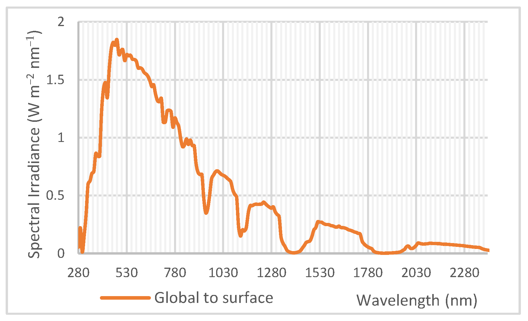
4.1. Downwelling Ambient Light

The level of radiance reaching the sea surface changes throughout the day, as well as throughout the seasons. The spectrum can be further impacted by cloud cover. The Sun’s azimuth and zenith angle at the location of interest changes due to the Earth’s rotation, axial tilt, and elliptical orbit around the Sun, causing the penetrating light rays to be refracted at an angle at the air–water boundary. This effect of the incidence angle is evident even in some of the earliest investigations of the underwater light field by Tyler [49] and later, Hoejerslev [50], where at a constant depth, the amount of light received was greatest when the receiver was directed toward the azimuth and zenith angles that corresponded to the refracted rays as per Snell’s law. However, these directional characteristics are lost with increasing depth as the light field transforms progressively from the “sunny condition” near the surface to a more diffuse distribution where ultimately, the peak radiance occurs at a receiver zenith angle of zero degrees, where it has reached its “asymptotic” form [48].

Furthermore, accurate site-specific downwelling spectral distribution is best obtained through in situ measurements, which can be resource intensive. Alternatively, historical data may be used, but would require rigorous analysis to forecast the spectra accounting for cloud cover and weather conditions for a given date. Instead, the SPCTRL2 model developed by Bird and Riordan [51] may be a good alternative to estimate the spectra based on date, time, location (latitude and longitude), and atmospheric data available in the public domain. Figure 4 shows that the global spectral distribution (including both direct and diffused sunlight incident at Earth’s surface) peaks in the blue-green region that also corresponds to the spectrum with the most penetrative ability underwater [39], thus raising questions of how significant this could contribute as optical noise.

The influence of lunar spectral radiance, on the other hand, may be considered less significant due to a smaller irradiation peak at about 5 mW m^™2, shifting toward the more attenuated amber-red spectrum for a full moon [53]. However, despite the lunar spectral variation being a less investigated topic, given that its spectrum also spans a bandwidth like the solar spectrum, it can be assumed that strategies that discriminate solar noise can also apply to lunar noise.

4.2. Stratified Oceans

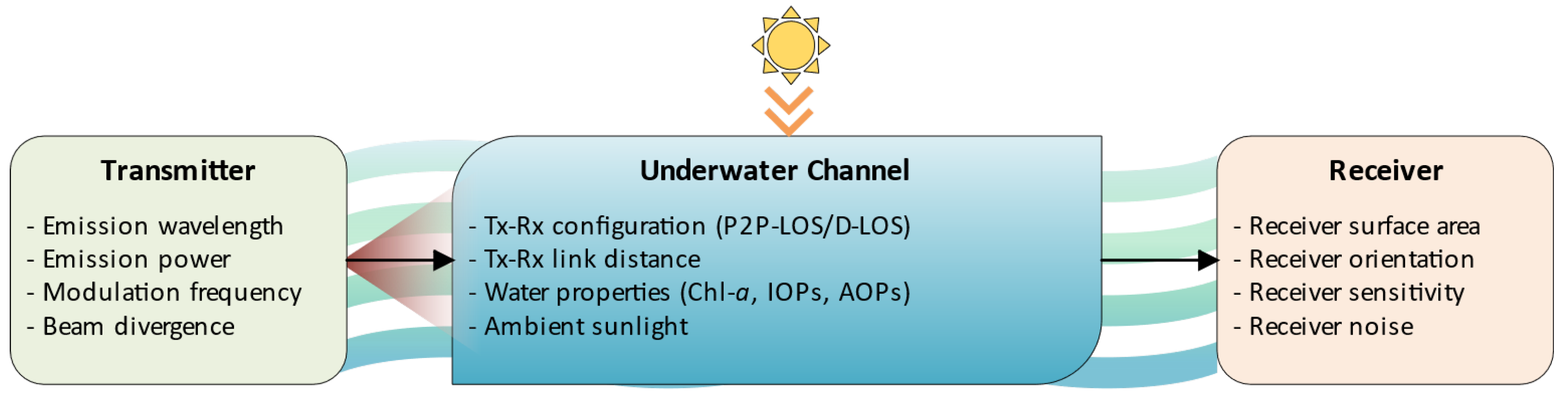
With respect to the availability of sunlight underwater, the ocean is divided into three zones. The euphotic zone is the uppermost section with an abundance of light and usually reaches a depth of about 200 m in clear waters. Beneath it is the disphotic zone, in which much of the yellow and red spectra have already been absorbed but blue-green spectra remain. This is typically 1 km deep. Beyond this is the aphotic zone, in which all downwelling light has diminished [54].

Due to the assumptions made in the determination of Jerlov types, modeling mobile UOWC performance using the coefficients reported by Jerlov would be unrealistic beyond a depth of about 10 m. Instead, the flexibility of modeling optical characteristics at a given ocean location or depth would be an ideal scenario.

Ocean color sensors on Earth observation satellites, such as the Sea-viewing Wide Field-of-view Sensor (Sea WiFS) and the Ocean Color and Temperature Scanner, have been used for a long time to monitor the distribution of chlorophyll-a (Chl-a) concentration at the sea surface, the principal pigment in chlorophyll [55]. Using these data, the vertical distribution of Chl-a concentration may be modeled [33,34,55].

Given the abundance of sunlight closer to the surface, chlorophyll concentration is primarily influenced by nutrient availability. However, with increasing depth and a lesser penetration of sunlight, photosynthesis is constrained, leading to a decrease in chlorophyll concentration. Within the transitional zone between sunlit, nutrient-poor waters and dark, nutrient-rich waters, a peak in chlorophyll concentration (deep chlorophyll maximum or DCM) is observed. The depth of this DCM typically falls within the range of 20 to 120 m, contingent on the surface concentration of chlorophyll [32,52]. The consistency of this phenomenon, described as a relative Gaussian distribution, has led to the development of models correlated with empirical data for the Chl-a concentration along a vertical column of water [55]. Furthermore, these models are consistent for oceans that are stratified, a very common occurrence, where the depth layers do not mix, thus enabling parameterization [34].

Uitz et al. have further extended this knowledge by classifying observations at 1821 stations across the globe into nine different ocean types: S1–S9, by order of surface Chl-a concentration (Figure 5) [34]. Their dimensionless parameterized Equation (5) and respective parameters are shown below and in

Table 2. Dimensionless normalized coefficients for vertical Chl-a concentration distribution [34].

Class	Cb	s	Cmax	ζmax	Δζ	${\stackrel{-}{\mathbf{C}\mathbf{h}\mathbf{l}\text{-}\mathit{a}}}_{{\mathbf{Z}}_{\mathbf{e}\mathbf{u}}}$	Zeu
S1	0.471	0.135	1.572	0.969	0.393	0.0910	119.1
S2	0.533	0.172	1.194	0.921	0.435	0.151	99.9
S3	0.428	0.138	1.015	0.905	0.630	0.185	91.0
S4	0.57	0.173	0.766	0.814	0.586	0.250	80.2
S5	0.611	0.214	0.676	0.663	0.539	0.338	70.3
S6	0.390	0.109	0.788	0.521	0.681	0.410	63.4
S7	0.569	0.183	0.608	0.452	0.744	0.578	54.4
S8	0.835	0.298	0.382	0.512	0.625	1.206	39.8
S9	0.188	0	0.885	0.378	1.081	2.950	26.1

, respectively, where $C_b$ is the surface chlorophyll concentration; $s$ is the vertical gradient of chlorophyll concentration; $\zeta$ is the dimensionless depth normalized for the euphotic depth $Z_{eu}$ in meters; $C_{max}$ is the Chl-a concentration at the depth ${\zeta }_{max}$ of the subsurface maximum; and ${\stackrel{-}{Chl\text{-}a}}_{Z_{eu}}$ is the average Chl-a concentration (mg m^™3) within the euphotic layer. This can be reconstructed into a dimensioned form $C_c(S,z)$ by using (6) and (7). S5–S8 are only plotted for a maximum depth of 110 m due to the Chl-a concentration approaching zero. It should also be noted that the characteristics of S9 cannot be modeled beyond shallow depths due to the fact that the value of ‘s’ given is 0 [34].

$$C_{DL}\left(\zeta \right)=C_b-s\zeta +C_{max}{e}^{-{\left[{\displaystyle \frac{\zeta -{\zeta }_{max}}{\mathsf{\Delta }\zeta }}\right]}^2}$$

(5)

$$C_c\left(\zeta \right)=C_{DL}\left(\zeta \right)\times {\stackrel{-}{Chl\text{-}a}}_{Z_{eu}}$$

(6)

$$z=\zeta \times Z_{eu}$$

(7)

Another parameterized version of these data, for Kameda and Matsumura’s equation, is presented by Johnson et al. [33], who have applied Haltrin’s single-parameter model based on Chl-a concentrations [56] for the derivation of attenuation subcomponents along the stratified column. This may be a more appropriate approach for estimating IOPs for practical situations, where georeferenced satellite information of surface Chl-a content could help to define the properties of the given water column. However, in this article, we have instead evaluated Chl-a concentrations using (5)–(7) and Table 1 from Uitz et al. [34] before applying Haltrin’s equations. For the re-parameterized coefficients, we refer the reader to Appendix A.

5. System Model

Seeking insights into enhancing the O-SNR requires investigating the performance of the UOWC by combining the existing UOWC signal propagative models with the distribution of downwelling light and vertical attenuation distribution, as presented in the previous section. Although there could be a relationship between the geographical location and the sunlight to the surface water Chl-a content [34], these have not been explored in this article. Instead, we apply the downwelling conditions to each of the ocean classifications S1–S8, along with UOWC propagative models, modeling for a worst-case scenario (daytime) for insights, as shown in Figure 6. The corresponding system modeling is presented here.

5.1. Haltrin’s Single-Parameter IOP Model Based on Concentration of Chlorophyll-a

Haltrin’s model is widely adopted for UOWC performance analyses, being derived from in situ measurements, which link the IOPs of seawater to the Chl-a concentration. It has been verified for Chl-a concentrations ranging between 0–12 mg m⁻³, within which are the concentrations of the profiles of stratified water bodies presented in Uitz et al. [56]. Prior to this model’s application, the depth $\left(z\right)$-dependent variation of Chl-a, $C_c(S,z)$, for each classification profile $S$, needs to be evaluated, as given in Section 4.2. The absorption coefficient $a\left(S,\lambda ,z\right)$ may be derived with (8), where $a_w\left(\lambda \right)$ is the pure water absorption coefficient adopted from Prieur et al. [57]; $a_c^0\left(S,\lambda ,z\right)$ is the specific absorption coefficient of Chl-a determined by (9) and the values for empirical constants A and B are available in Pope and Fry [58]; $C_c^0$ is the total reference concentration of Chl-a (1 mg m⁻³); $a_f^0$ is the specific absorption coefficient of fulvic acid at 35.959 m² mg⁻¹; $k_f$ = 0.0189 nm⁻¹; $a_h^0$ is the specific absorption coefficient of humic acid at 18.828 m² mg⁻¹; $k_h$ = 0.01105 nm⁻¹; and $C_f$ and $C_h$ are the concentrations of fulvic and humic acids in mg m⁻³, calculated using (10) and (11), respectively.

$$a\left(S,\lambda ,z\right)=a_w\left(\lambda \right)+a_c^0\left(S,\lambda ,z\right){\left({\displaystyle \frac{C_c\left(S,z\right)}{C_c^0}}\right)}^{0.602}+a_f^0{C}_f\left(S,z\right)e^{-k_f\lambda }+a_h^0{C}_h\left(S,z\right)e^{-k_h\lambda }$$

(8)

$$a_c^0\left(S,\lambda ,z\right)=A\left(\lambda \right){C_c\left(S,z\right)}^{-B\left(\lambda \right)}$$

(9)

$$C_f\left(S,z\right)=1.74098C_c\left(S,z\right)e^{0.12327\left({\displaystyle \frac{C_c\left(S,z\right)}{C_c^0}}\right)}$$

(10)

$$C_h\left(S,z\right)=0.76284C_c\left(S,z\right)e^{0.03092\left({\displaystyle \frac{C_c\left(S,z\right)}{C_c^0}}\right)}$$

(11)

Note that the above models and the following are computable only for the 400–700 nm range limited by the coefficient availability in the reference studies. However, this is sufficient as this bandwidth covers a full span of the visible spectrum used in UOWC due to limitations posed by attenuation (wavelengths less than 400 nm or greater than 700 nm are highly attenuated in seawater) and hardware (semiconductor photodetectors are much less sensitive to wavelengths less than 400 nm).

The scattering coefficient $b\left(S,\lambda ,z\right)$ is derived from (12), where $b_w\left(\lambda \right)$ is the scattering coefficient of pure water calculated with (13); $b_s^0\left(\lambda \right)$ and $b_l^0\left(\lambda \right)$ are the specific scattering coefficients of small and large suspended particles, respectively, in m² g⁻¹; and $C_s\left(S,z\right)$ and $C_l\left(S,z\right)$ are the concentrations of small and large particles in g m⁻³, calculated using (16) and (17), respectively.

$$b\left(S,\lambda ,z\right)=b_w\left(\lambda \right)+b_s^0\left(\lambda \right)C_s\left(S,z\right)+b_l^0\left(\lambda \right)C_l\left(S,z\right)$$

(12)

$$b_w\left(\lambda \right)=0.005826{\left({\displaystyle \frac{400}{\lambda }}\right)}^{4.322}$$

(13)

$$b_s^0\left(\lambda \right)=1.151302{\left({\displaystyle \frac{400}{\lambda }}\right)}^{1.7}$$

(14)

$$b_l^0\left(\lambda \right)=0.341074{\left({\displaystyle \frac{400}{\lambda }}\right)}^{0.3}$$

(15)

$$C_s\left(S,z\right)=0.01739C_c\left(S,z\right)e^{0.11631\left({\displaystyle \frac{C_c\left(S,z\right)}{C_c^0}}\right)}$$

(16)

$$C_l\left(S,z\right)=0.76284C_c\left(S,z\right)e^{0.03092\left({\displaystyle \frac{C_c\left(S,z\right)}{C_c^0}}\right)}$$

(17)

Backscattering may be determined using (18), where $B_s$ (0.039) and $B_l$ (0.00064) are the probabilities of scattering by small and large particles, respectively. It is needed for the evaluation of underwater reflectance; an AOP used in modeling ambient light.

$$b_B\left(S,\lambda ,z\right)={0.5b}_w\left(\lambda \right)+{B_{s}b}_s^0\left(\lambda \right)C_s\left(S,z\right)+{B_{l}b}_l^0\left(\lambda \right)C_l\left(S,z\right)$$

(18)

The linear sum of $a\left(S,\lambda ,z\right)$ and $b\left(S,\lambda ,z\right)$, as in (1), is used to determine the spectral attenuation $c\left(S,\lambda ,z\right)$ for each profile. Figure 7 shows the depth–spectral distribution of attenuation for profiles S2 and S8.

5.2. Ambient Noise

The downwelling irradiance ($E_t$) is the integral of all spectral irradiances in W m⁻² (radiometric), expressed in (19). The background power experienced by a receiver of surface area $A_r$ is derived using (20).

$$E_t=\int E\left(\lambda \right) d\lambda$$

(19)

$$P_{BG}\left(S,\lambda ,z\right)={\displaystyle \frac{\pi A_r{\Omega }^2{T}_f{\int }_{\mathsf{\Delta }}\left(L_{sol}\left(S,\lambda ,z\right)+L_{bb}\left(S,\lambda ,z\right)\right) d\lambda }{4}}$$

(20)

where $\Omega$ is the plane angle of the field-of-view (FOV) of the receiver in radians, $T_f$ and $\mathsf{\Delta }$ are the optical filter transmissivity and bandwidth, respectively, $L_{sol}$ is the upwelling solar spectral radiance, and $L_{bb}$ is the blackbody radiation of the water body. $c_d$ is the diffuse attenuation coefficient, an AOP that describes how a background light field may attenuate in water expressed from IOP using (21) [31]. Equation (4), which corresponds to the light intensity at a location, may be thereafter adapted for the attenuation of downwelling irradiance in a stratified environment using (22), where $n$ is a layer of unit depth in meters and $z$ is the receiver depth. Therefore, $L_{sol}$ may be derived for each profile with (23), where $R_f$ is the underwater reflectance that expresses a ratio between downwelling and upwelling irradiances correlated to the backscattering coefficient with (24) [59]. $L_f$ is the radiance factor, expressed as the ratio between the radiance observed at an angle of interest (receiver orientation) with respect to the nadir, or looking vertically down. The corresponding values for a horizontal link and downlink (receiver looking up) were extracted from the sources for oceanic (S1–S4) and coastal (S5–S8) waters from Duntley [48], Hoejerlev and Aas [50], and Aas and Hoejerslev [60].

$$c_d\left(S,\lambda ,z\right)\approx {\displaystyle \frac{c(S,\lambda ,z)}{3}}$$

(21)

$$E_t={\int }_{\mathsf{\Delta }}{E}_0(\lambda )\prod _{n=1}^z{e}^{-c_d\left(S,\lambda ,z_n\right)} d\lambda$$

(22)

$$L_{sol}\left(S,\lambda ,z\right)={\displaystyle \frac{{E_0\left(\lambda \right)R}_f\left(S,\lambda ,z\right)L_f\prod _{n=1}^z{e}^{-c_d\left(S,\lambda ,z_n\right)}}{\pi }}$$

(23)

$$R_f\left(S,\lambda ,z\right)\approx {\displaystyle \frac{b_B\left(S,\lambda ,z\right)}{3a\left(S,\lambda ,z\right)}}$$

(24)

Blackbody radiation is described as the EM radiation emitted by an object at a particular temperature on the Kelvin scale, idealized for a perfect black object. It is expressed by (25), where $h$ is Planck’s constant (6.626 × 10⁻³⁴ J s), $v$ is the speed of light in water (2.253 × 10⁸ m s⁻¹), $k_B$ is the Boltzmann constant (1.381 × 10⁻²³ J K⁻¹), $T$ is the temperature of the body in Kelvin, and $\alpha$ is the radiance absorption factor (0.5) [19]. Given that the underwater environments are about 300 K or lower, much of this radiation available is in the infrared spectrum.

$$L_{bb}\left(S,\lambda ,z\right)={\displaystyle \frac{2h{v}^2\alpha }{{\lambda }^5 \left(e^{\left(\frac{hv}{k_{B}T\left(S,z\right)}\right)}-1\right)}}$$

(25)

5.3. Geometric Propagation Models Common for UOWC

In addition to the models for attenuation distribution and downwelling light, the geometric models that describe the optical signal propagation underwater need to be determined. This is dependent on the type of transmitter (Tx)–receiver (Rx) link configuration: a point-to-point line-of-sight (P2P-LOS) or diffused line-of-sight (D-LOS). In P2P-LOS connections, the Tx emits a focused beam at small beam divergence angles ($\theta$ rad). However, despite such links achieving greater link distances, they are prone to misalignments due to the small beam area and require complex optical systems to maintain connectivity. In D-LOS links, on the other hand, the transmission beam covers a wide region, as for example, from a LED array. They are more suitable for mobile links due to less demanding alignment needs, but they suffer more losses due to geometric spread. The expressions for beam coverage ($A_s$ m²) for P2P-LOS and D-LOS are given in Equation (26), where $d$ is the distance of the link.

$$A_s=\left\{\begin{array}{c}\pi {\left(d\tan \mathsf{\theta }\right)}^2 \left(\mathsf{\theta }\ll {\displaystyle \frac{\pi }{20}}\right)\\ 2\pi d^2\left(1-\cos \mathsf{\theta }\right) \left(\mathsf{\theta }>{\displaystyle \frac{\pi }{20}}\right)\end{array}\right.$$

(26)

For horizontal links, the attenuation factor may be adopted directly from Equation (4). For downlinks experiencing stratification, the vertical link distance $d$ becomes the difference in depth between the depth position of the Tx ($z_0$) and Rx ($z$), assuming the Tx is directly above the Rx to allow for a worst-case noise scenario at the Rx, expressed in Equation (27). The optical power received at the receiver $P_r\left(S,\lambda ,z\right)$ can then be determined for horizontal and vertical links with Equation (28), where $P_t\left(\lambda \right)$ is the spectral emission power in watts and $\phi$ is the sum of the angles of inclination ($\alpha$) and rotation ($\beta$) of the receiver with respect to the emitter’s axis (29).

$$d=\left\{\begin{array}{c} d \left(\mathrm{h}\mathrm{o}\mathrm{r}.\right)\\ z-z_0 \left(\mathrm{v}\mathrm{e}\mathrm{r}.\right)\end{array}\right.$$

(27)

$$P_r\left(S,\lambda ,z\right)=\left\{\begin{array}{c}{\displaystyle \frac{P_t\left(\lambda \right)A_r\cos \phi e^{-c\left(S,\lambda ,z\right)d}}{A_s}} \left(\mathrm{h}\mathrm{o}\mathrm{r}.\right)\\ {\displaystyle \frac{P_t\left(\lambda \right)A_r\cos \phi \prod _{{n=z}_0}^z{e}^{-c\left(S,\lambda ,z_n\right)}}{A_s}}\left(\mathrm{v}\mathrm{e}\mathrm{r}.\right)\end{array}\right.$$

(28)

$$\phi =\alpha +\beta$$

(29)

5.4. Optical SNR

The SNR for a communication system is a key indicator for how well the link will perform—the higher the SNR, the better. The SNR for UOWC is generally estimated as the ratio of signal power to the sum of noise power by ambient light, dark current (the leakage current in the PD), shot noise (a portion of signal that contributed to noise), and thermal noise (from passive electronic devices such as the preamplifier circuits). Given that the objective of this study is to shed light on the considerations from a physical layer perspective for maximizing the SNR of UOWC, the inclusion of noise by the preamplifier circuitry was not included and the resulting SNR was determined as an O-SNR. This is due to the preamplifier effects being significantly determined by an engineer’s design choices, which is difficult to standardize for such a model.

The noise due to ambient light (${\sigma }_{BG}^2$) may be expressed with Equation (30), where $q$ is the electronic charge (1.602 × 10⁻¹⁹ C), $S_r\left(\lambda \right)$ is the spectral variation in the responsivity of the PD in A/W, and $B$ is the signaling bandwidth in Hz. The effect of dark current (${\sigma }_{DC}^2$) is expressed in Equation (31), where $I_{DC}$ is the dark current, retrievable from the datasheet of the PD, in amperes. The shot noise (${\sigma }_{SS}^2$) is given in Equation (32). The signal bandwidth will be limited to a 3 dB frequency bandwidth of the PD, as it suggests the upper limit possible for any modulation signal, either by a LED or a laser, and is given by Equation (33), where $t_R$ is the rise time of the PD as available from the datasheet.

$${\sigma }_{BG}^2\left(S,\lambda ,z\right)=2q{S}_r\left(\lambda \right)P_{BG}\left(S,\lambda ,z\right)B$$

(30)

$${\sigma }_{DC}^2=2q{I}_{DC}B$$

(31)

$${\sigma }_{SS}^2\left(S,\lambda ,z\right)=2q{S}_r\left(\lambda \right)P_r\left(S,\lambda ,z\right)B$$

(32)

$$B\approx {\displaystyle \frac{0.35}{t_R}}$$

(33)

Therefore, the overall optical noise $\left({\sigma }_{Opt}^2\right)$ can be expressed with Equation (34), and the final O-SNR with Equations (35) and (36).

$${\sigma }_{Opt}^2={\sigma }_{BG}^2+{\sigma }_{DC}^2+{\sigma }_{SS}^2$$

(34)

$$O\text{-}SNR={\displaystyle \frac{{\left(S_r\left(\lambda \right)P_r\left(S,\lambda ,z\right)\right)}^2}{{\sigma }_{Opt}^2\left(S,\lambda ,z\right)}}$$

(35)

$$O\text{-}SNR={\displaystyle \frac{{S_r\left(\lambda \right)}^2{P}_r^2\left(S,\lambda ,z\right)}{2qB\left(I_{DC}+S_r\left(\lambda \right)P_r\left(S,\lambda ,z\right)+S_r\left(\lambda \right)P_{BG}\left(S,\lambda ,z\right)\right)}}$$

(36)

6. Simulation and Parameters

6.1. Transmitter and Receiver Parameters

The transmitter parameters were designed to be arbitrary inputs for which the UOWC performance was simulated. The model determines the O-SNR outcome of a link at a given power and beam divergence angle (for D-LOS and P2P-LOS links) for all wavelengths in the 400–700 nm spectra (2.5 nm bandwidth resolution) for any correlations between the parameters and noise influences, while also varying the depths and link distances as detailed in Section 6.2. Section 7 discusses the UOWC performance for selected parameters of beam divergence angles of 120°, 60° (D-LOS), and 5° (P2P-LOS). The transmission powers were set to 1 W and 10 W, as made possible by off-the-shelf emitters.

The receiver photodiode was a blue-green wavelength enhanced First Sensor PIN-PD (Model: PS13-6b TO PD) with hardware parameters as given in

Table 3. List of physical parameters of the PIN photodiode used in the model [61].

Parametar	Typical Value	Unit
$\mathrm{Active} \mathrm{area} (A_r$)	13	mm2
$\mathrm{Dark} \mathrm{current} (I_{DC}$)	0.25	nA
$\mathrm{Rise} \mathrm{time} (t_R$)	70	ns
$\mathrm{FOV} (\Omega$)	tan−1 (6.1/4.84)	rad.

[61]. The spectral responsivity curves were extracted from the datasheet. This device was selected due to the high 3 dB frequency bandwidth of approximately 5 MHz, large active area, and broad spectral responsivity. Given that large active regions correlate to lower response times, this device seemed to provide a good trade-off between the received power while maintaining a frequency response that could still accommodate for multimedia transmissions.

6.2. Downlink and Depth-Variant Horizontal Link

Although mobile UOWC links are oblique in nature, results for a worst-case scenario (receiver looking directly above) and typical scenario (horizontal) can establish insights for the intermediate configurations.

In the vertical scenario, the transmitter depth $z_0$ is varied by distinct intervals of unit depths as seen in Figure 8a, and the corresponding O-SNR is modeled for vertical depth, wavelength, transmit power, and beam divergence. In the horizontal scenario, the transmitter depth $z$ is varied by distinct intervals as seen in Figure 8b, and the corresponding O-SNR is modeled for horizontal distance, wavelength, transmit power, and beam divergence.

6.3. Simulation

The simulation was conducted using MATLAB. First, the horizontal UOWC link configuration (Figure 8a) was simulated for a “night” condition, with no downwelling sunlight. This would show link behavior as such when only attenuation was the link determining factor. Possible lunar radiation was not applied due to reasons mentioned in Section 4.1. Thereafter, each water profile was simulated with sunlight for the configurations shown in Figure 8a,b. S1–S4 were modeled for a depth of 250 m, and S5–S8 up to 110 m, due to Chl-a concentrations reaching near zero. Given these depths are below the DCM, they are sufficient for observing the nuanced characteristics of the profiles. The horizontal link distance was simulated up to about 100 m for D-LOS links and about 300 m for P2P-LOS links, seen in the results to be the sufficient upper limit for link lengths. S9 was not modeled due to its lack of completeness in parameterization with its Chl-a concentration data from just 18 samples being limited to the near-surface water [34], but observations made for S8 as the next most coastal profile, may be extended for S9. Reflections at the air–water boundary were not included due to it being a non-line-of-sight path, which may contribute to both noise and gain depending on the delay spread, which is a consideration in modulation, not in the scope of this analysis. The sun was assumed to be at zenith, directly above the ocean surface. This negated the peaking of the underwater radiance at the solar azimuth at shallow depths, which would have caused the receiver to experience more light facing toward this direction and lesser light when turned away for the horizontal UOWC link configuration compared to the average value this model assumes. This was due to the lack of radiance data that corresponded to these water profiles to model otherwise. Despite it, this is a reasonable assumption, given that the underwater radiance reaches an “asymptotic form” with increasing depth, where the light field becomes increasingly diffuse and peaks at the zenith [48]. The 10 nm bandwidth resolution from SPCTRL2 was interpolated to a resolution of 2.5 nm, the minimum resolution to which coefficients in Section 5.1 were evaluated for. Results have been discussed for S1 (most clear ocean), S4 (least clear ocean), S5 (least coastal) and S8 (most coastal profile). Blackbody radiation was not included in this model because this radiation peaks in the IR spectrum for an ambient temperature of 300 K and spectral magnitudes less than 1% of the typical noise-equivalent power of the PD of 4 × 10⁻¹⁴ W/√Hz, suggesting an insignificant contribution as noise. We asked two questions. Firstly, how does changing emission parameters such as transmit power and beam divergence angle at each wavelength in the visible spectrum affect the overall O-SNR observed at the receiver under changing attenuation and sunlight conditions for horizontal and downlink orientations? Secondly, for a given set of transmission parameters, could altering the transmission wavelength help achieve longer link establishment distances in these environments, and if so, what is the observed trend?

7. Results and Discussion

The downwelling solar spectral irradiance modeled under the influence of the stratified water column (Figure 9a,d) shows a substantial availability of the blue-amber spectrum with depth, irrespective of the level of clarity of the water. As expected, the blue-green bandwidth is more prominent in the clear seawaters of S1 (approx. 25 mW m⁻² at 250 m depth), whereas in the highly coastal S8, the green-amber spectrum is more abundant (approx. 0.25 mW m⁻² at 100 m depth), both of which are significant intensities that could contribute as noise. However, in the determination of ambient noise power (Figure 9b,e), the power is significantly higher toward the shorter wavelengths in the clear waters than the coastal profiles in both vertical and horizontal orientations. The resulting effect of this influence can be explained effectively by separating the UOWC outcome into depths above the DCM and depths below it, as discussed in Section 7.2. In Section 7.1, we first investigate the “no light” condition for horizontal UOWC links, where depth-variant attenuation is the main contributor of varying channel conditions.

7.1. Simulation Results with No Sunlight

Considering the D-LOS results, in the clearest water profile S1 (Figure 10a–d), it is seen that the best wavelengths for links under 30 m seems to be in the blue-green region. This is most prominent in depths closer to the DCM. However, above and below the DCM, it is seen that even the deeper blue wavelengths are preferred for longer horizontal links. However, with decreasing profile clarity, the depths above the DCM seem to shift this preference also to the blue-green region as seen in all results of S4 (Figure 10e–h), and then to the yellower wavelengths as seen in the S8 profile (Figure 10m–p).

It is visible that for very short D-LOS links, yellow was preferable for all water profiles with increasing turbidity. Yellow is also preferable at slightly longer link distances within the same profile where the geometric loss of signal was greater. This could be attributed to the generally higher photodiode responsivity for longer wavelengths, until such distances where the higher attenuation of the yellow-amber spectrum in clearer waters would cause this spectrum reception to diminish compared to the blue-green wavelengths. The maximum achievable 0 dB distance (the magenta-colored line) seems to decline for all water profiles approaching the DCM. The maximum distance reached below the DCM seems to be greater than above it (S1–S8). This is due to the Chl-a concentrations reaching a near-zero value, which is much less than above the DCM. Furthermore, the reason why the more turbid profiles seem to achieve greater 0 dB distances at shallower depths could be explained also by the steeper decline of the Chl-a concentrations (Figure 5) and the dominant contributor to the attenuation is then eventually only seawater.

Observing the P2P-LOS results (Figure 11), we further see that a bluer spectrum is favored for the clear water profiles, which shifts to greener spectra with increasing turbidity. S8 (Figure 11d,h) is an exception due to its very high turbid conditions in the shallower depths causing very high scattering, and thus there is lesser attenuation of the yellow-amber spectrum there. As expected, the 0 dB link distances (Figure 11a–h) are much greater than they were for the D-LOS profile results. These overall observations could be due to the very low geometric losses caused due to the narrow beam divergence angle of the emitter.

7.2. Simulation Results with Sunlight

For D-LOS horizontal links approaching the DCM, there seems to be a surprising preference for the yellow-amber spectrum for O-SNR (Figure 12a–p) in short-range horizontal links at an average of 25 m or less, in all profiles S1–8, in the upper depth layers. The color preference then alters to green and then blue (with increasing depth) in accordance with the attenuation curves. In P2P-LOS horizontal links (Figure 12q–x), although this yellow preference exists for more coastal profiles, the link lengths are very short and mostly at the level of the DCM. However, for the P2P-LOS clear profiles S1–S4, it is seen that the green wavelengths are preferred more for the depths above the DCM for the sunlit condition than for the night condition. Note that, in the coastal S5, the profile with a 1 W emitter shows an increasing preference for yellow wavelengths closer to its DCM, but this is minimized to a small elliptical region in the 10 W profile, suggesting that the choice of transmission power has a role to play. This is justified when observing that all 120° D-LOS profiles have greater yellow-amber regions than their 60° counterparts. This is due to the high geometric losses which have highlighted the yellow-amber spectrum for short link lengths due to being at a higher energy than sunlight’s yellow-amber spectrum at these distances. However, due to experiencing higher attenuation, it is then succeeded by the green spectrum with increasing Tx–Rx distance. The greater penetration and availability of sunlight could be the possible reasoning behind why the clear profile S1 shows a greater yellow-amber region than S4: because even though the attenuation distributions for both are the lowest in the blue-green spectrum, the ambient blue-green spectrum in S1 experiences lesser degradation than S4 due to the deeper positioning of the DCM and the lower Chl-a concentration overall, and therefore is more abundant in the S1 profile.

The explicit behavior of the S8 horizontal profiles which consistently showed a yellow-amber layer above the DCM, but below it gradually shifted to green and blue wavelengths, could be explained by referring to its attenuation profile (Figure 7b) that shows a big dip in the attenuation distribution in the amber spectrum at shallower depths but shifting to the blue-green region progressively below the DCM. Due to this, although the transmission parameters may have had some causality, the observations have been overshadowed by the effect from the attenuation profile, and thus may not display a preference based on horizontal link distance. This characteristic is also visible in other coastal profiles, but to a lesser effect due to a less comparable dip in the attenuation coefficient in the yellow-amber spectrum compared with S8. However, as a general trend, the depth of the yellow-amber preferred region is shifted vertically up and extended horizontally for all profiles with an increasing level of turbidity. The lateral observations could be due to the compounded effects of the relatively lesser abundance of the yellow-amber spectrum in downwelling sunlight compared to the blue-green spectrum, the preference of the yellow-amber region in the attenuation curves with increasing turbidity in the shallower regions, and the greater responsivity of the photodetector to these wavelengths, thus achieving longer link lengths there.

The preference for shorter wavelengths overall with increasing depth can be explained by considering that the ambient sunlight gets attenuated and filtered in the upper layers, especially in the coastal profiles, where the DCM is closer to the ocean surface, thus promoting the blue-green spectrum for transmission in the lower layers for a higher O-SNR.

In addition to the wavelength of preference for the maximum O-SNR, it is also essential to estimate the wavelength of preference for link establishment. This is the wavelength at each layer in the stratified water column that achieves the greatest horizontal distance (0 dB distance), where the signal and noise are indistinguishable (the spectral distributions for D-LOS links are given in Figure 13a–p and for P2P-LOS in Figure 13q–x). This corroborates directly to the magenta-colored lines in Figure 12 which show the 0 dB distance at the given depth, where the color beneath is the carrier wavelength that achieves it. The determination of the best O-SNR wavelength helps to determine what wavelength is necessary to achieve the best signal quality at a given depth and distance, but determining the wavelength for maximum distance shows the condition for link establishment from a range perspective. These two considerations are distinct due to the link length (Figure 13) predominantly showing the finite limits possible, while the O-SNR (Figure 12) is determined by the ratio of signal power to noise present at any given location within this limit, where a different light wavelength may be favorable for communication due to experiencing lesser attenuation or having less downwelling light of that spectrum from sunlight. This can yield insights for modulation strategies, where for example, an OOK-based link that needs a SNR of 10–20 dB would prefer a much more drastic wavelength variation with depth.

It is clearly seen in the clear water profiles S1–S4 in Figure 12 that for the high-power systems ($\theta$= 120°, 10 W, Figure 12d,h,l,p), ($\theta$= 60°, 10 W, Figure 12b,f,j,n), and ($\theta$= 5°, 10 W, Figure 12u–x), at shallow depths before the DCM, the best wavelengths for link length shift from amber-green to green-blue with increasing transmission power. This is due to the signal overcoming the significance of solar influence. This is confirmed as we look at their low power counterparts: ($\theta$= 5°, 1 W, Figure 12q–t), ($\theta$= 60°, 1 W, Figure 12a,e,i,m), and ($\theta$= 120°, 1 W, Figure 12c,g,k,o); in order of decreasing power, the wavelength for peak distance shifts from blue-green to amber. Therefore, a general suggestion is that using emissions of approximately 10 W with narrow beam divergences in the blue-green wavelengths may be optimal for clear water profiles. However, this is specifically under the sunlight profile shown in Figure 4. Nevertheless, the coastal profiles S5–8 seem to show a greater preference for the green-amber spectrum across all transmission powers at depths above the DCM. Also, as a general trend, the range limit at depths approaching the DCM decreases with increasing turbidity.

All horizontal link profiles for S1–8 seem to prefer the yellow-amber spectrum at the DCM depth under sunlight, with the clearer waters achieving the greatest link lengths above it (at those spectra previously mentioned), steeply declining toward the DCM before increasing again. Furthermore, the level of this decline reduces with increasing turbidity from profiles S1–8, respectively. Below the DCM, the favorable spectra for S1–8 shifts toward blue with increasing depth and achieves greater link lengths than above the DCM. The more coastal profiles seem to achieve greater link lengths at shallower depths from the depth position of the DCM.

In the downlink for D-LOS (Figure 14) and P2P-LOS (Figure 15) links, the preferred wavelength at close-range links has shifted to the yellow-orange spectrum, and even to red in low-power D-LOS (1 W at $\theta$= 60°, Figure 14a,e,i,m and $\theta$= 120° at both power settings, Figure 14c,g,k,l,o,p) approaching the DCM. This can be due to the direct view of downwelling sunlight on the receiver when it is facing up. The amber range is about 20–50 m for the clearer water S1, and grows as the depth approaches the DCM, maintaining this trend for depths beyond the DCM due to more sunlight penetration. The more coastal profiles show a much greater amber region toward the surface like their horizontal link profiles.

These observations for both downlinks and horizontal links under Chl-a concentration profiles show that the transmission wavelength has a significant role in the determination of the signal quality and range in the presence of sunlight, which dynamically changes based on the position and orientation of the Tx and Rx within a given stratified environment, in addition to the properties of the environment itself being determined by the surface Chl-a concentration. It shows that for the maximum performance for a moving link, a broader wavelength spectrum should be considered for the carrier determined based on the water profile, time of day, depth, and link distance. This raises a problem with narrowband wavelength transmissions from emitters limited to a few tens of nm for LEDs and <10 nm for lasers, suggesting that a more dynamic scheme of signaling may be necessary that is responsive to the channel state information (CSI) parameters that include localization information. Nevertheless, to some extent, using the green spectrum at transmission powers over 10 W and narrow beam divergence angles may seem like an overall solution. However, this could be demanding on the power budget of the autonomous UOWC nodes that are better reserved for other tasks. Such narrow links may also suffer misalignment. Additionally, for example, 10 W lasers are highly hazardous and may harm marine animals. They may also not be a viable solution for mobile links where large beam divergences are preferred, such as in wireless networks and swarms, where the results show persisting disturbance from sunlight. In such cases, it seems gradually shifting the transmission wavelengths to the yellow-amber spectrum as the day approaches could be a strategy. However, this is contingent upon many factors, such as geographic location, season, cloud cover, etc. For example, conducting the analyses nearer to the equator may result in a greater preference for the yellow-amber spectrum due to greater availability of sunlight.

This study, considering a wavelength resolution of 2.5 nm, further verifies that just the use of bandpass optical filters without any additional special discriminatory characteristics may not be an effective solution due to the downwelling solar spectra encompassing the full visible light spectrum used in UOWC. Instead, for example, a scheme such as differential signaling that incorporates two or more emission spectral bands could be more effective, where a choice of green and yellow wavelengths may benefit link length and the SNR. Where multiple links are to be established, such as for swarming, a depth- and distance-based wavelength division multiplexing scheme may be effective, where a separate wavelength is assigned for bands of distances from the transmitter. This study also provides preliminary insights beneficial for routing operations, where cooperative links would need to shift between carrier wavelengths for maximum performance based on the node depth and intermediate link distances. It also appears more favorable to route through paths beneath the DCM, where transmission distance is a priority or the number of intermediate nodes is limited. This could provide an alternative solution to the issues faced in cooperative UOWC faced by Xing and Yin [62], where their strategy for using shallow-water surface reflections were significantly affected by sunlight.

It should further be noted that no modulation scheme was implemented in this analysis, which means that the maximum achievable link lengths as per the modulation scheme will depend on several factors, such as the modulation scheme itself and the bandwidth, dependent on the overall SNR and at which distance is often considered where the forward error correction rate is approximately $3.8\times {10}^{-3}$ on a bit error plot. This distance is expected to be less than that represented by the magenta-colored line for the horizontal profiles. Another limitation of this study is the non-inclusion of the transimpedance circuitry, due to it being an engineering choice, that would have introduced Johnson noise into the system from the gain resistance. However, given that the Johnson noise from an ideal preamplifier of infinite gain is a negligible value, we determine that our findings hold true for this scenario. Furthermore, the variation in salinity gradients and turbulence across the vertical channel have not been implemented in this study for the purpose of limiting the scope of this current work. This is due to its impacts mainly affecting the beam alignment due to refraction in P2P-LOS links with much smaller beam divergent angles with lasers than assessed here $\left(\mathsf{\theta }\ll {\displaystyle \frac{\pi }{20}}\right)$. Additionally, the perspective of this work was to highlight how choosing an optimal light wavelength could result in a higher SNR. To further limit its impacts, we only considered perfectly horizontal and vertical link establishments. Under the considered stratification model, the horizontal beam travels through the same medium composition and the vertical beams will have an AOI of 0° to the stratified layers, thus passing straight through without refraction. Furthermore, the key insights of this study are associated with D-LOS links, where link misalignments have little impact. In waters where salinity and turbulence effects may be prominent, modulation-based strategies, as demonstrated by Chaudhary et al., may be explored to mitigate the effects [63].

We adopted SPCTRL2 to model sunlight due to its relative simplicity for generating the solar spectrum based on location and atmospheric information easily available in the public domain. This is a matter of convenience for on-the-go engineering needs. Where a more accurate spectra are necessary and specific information such as atmospheric aerosol concentrations are available, we refer the reader to more sophisticated models such as SMARTS2 [64,65] or MODTRAN [66], a highly complex tool used by researchers and government agencies.

Nevertheless, given that the results of this study apply to a fundamental determinant of UOWC, i.e., the carrier, it will therefore apply to all modulations and multiple-access schemes regardless. These results further highlight an additional layer of complications to consider upon the findings of Waduge et al. that showed how the effects of geometric loss and attenuation created spatial variability in the received optical power, with implications for modulation schemes and receiver array designs [67].

Validating the findings of this study at scale may be extremely resource intensive. However, it may be possible to simulate the conditions in a scaled version using a solar simulator and a partitioned water tank to introduce stratification. Absorption and scattering qualities could be introduced using agents such as Nigrosin dye and Maalox antacid [68]. Critical design decisions will need to be made to prevent total internal reflection within each partition. It is preferable that a high-end solar simulator is selected that produces a class-A spectral match. Alternatively, conducting a partial simulation-based study may be more effective by gathering vertical Chl-a concentration profiles and the solar spectral distribution in the field, then simulating with established UOWC geometric models to estimate the O-SNR. However, to our knowledge, it has been difficult to find datasets with both Chl-a and solar spectral information collected during the same voyage, which is a crucial factor for such a study. Furthermore, the schemes to discriminate these effects may be addressed from a signaling or hardware point of view and must be verified through additional studies (mobility models, etc.). We aim to explore these in our future works.

8. Conclusions

The quality of an underwater mobile optical wireless communication link is determined by several time-varying factors from downwelling sunlight to changing attenuation levels in inhomogeneous vertical channels, making the determination of optimal UOWC link parameters challenging. In this study, we focused on how optimal light wavelengths can enhance the SNR in such environments for horizontal and vertical links. We used MATLAB to conduct the numerical modeling for a holistic and realistic integration of the influence of sunlight on eight different vertically stratified ocean types in increasing order of turbidity, deriving the IOPs from the depth distribution of Chl-a concentration. Thereafter, UOWC has been simulated under the varied key transmission parameters of wavelength, output power, and beam divergence angle for a horizontal link (general case) and a downlink (worst case) for insights into any co-dependencies. The results showed a significant influence of the full sunlight spectrum in the upper layers of all seawater profiles with a deeper penetration of the blue-green solar spectrum in clearer oceans. Regarding the optimal transmission wavelengths for the SNR, this is further contingent upon the magnitude of geometric loss and node positioning with reference to the deep chlorophyll maximum. It is favorable to use the yellow-amber spectrum in a short range in coastal waters at all depths above the DCM, and for above-DCM links in clear oceanic waters that experience greater geometric loss. This spectrum advantage shifts to the blue-green spectrum with increasing depth for clear oceanic and coastal profiles. However, under solar influence, blue-green links established in the deeper layers of coastal profiles seem to show higher SNRs than clear oceanic profiles of same depth, possibly due to filtering out sunlight in the upper layers that are more abundant with Chl-a. The maximum achievable link range decreased approaching the DCM prior to increasing again.

We considered perfectly horizontal and vertical links, not accounting for salinity gradients, turbulence, or reflections at the air–water boundary. We assumed the sun was at zenith, vertically above the water surface, acknowledging that this neglects the peaking of light intensity in specific directions at very shallow depths due to the effect from solar zenith and azimuth angles. Additionally, while SPCTRL2 was used for its simplicity, more advanced solar spectrum models may be used for accuracy where certain specific non-public domain information about the locations of interest are available.

The findings suggest that UOWC-based sensor networks would benefit from adapting the carrier wavelengths to optimize for the node location, link distances, ocean type, and time of day, especially if they are within the photic region. Consequently, we propose wavelength-based modulation and routing strategies to discriminate the influence of sunlight. This study will further benefit from experimental validation. We intend to explore these in our subsequent research work.

References

1. Rayner, R.; Jolly, C.; Gouldman, C. Ocean observing and the blue economy. Front. Mar. Sci. 2019, 6, 330. [Google Scholar] [CrossRef]
2. Walsh, D. Exploration and technology—Key building blocks for the new blue economy. In Preparing a Workforce for the New Blue Economy; Elsevier: Amsterdam, The Netherlands, 2021; pp. 3–16. [Google Scholar]
3. Graham, A.; Marouchos, A.; Martini, A.; Fischer, A.; Seet, B.-C.; Guihen, D.; Williams, G.; Symonds, J.; Ross, D.; Soutar, J.; et al. Autonomous Marine Systems at Offshore Aquaculture and Energy Sites; 1.20. 002–Final Project Report; Blue Economy CRC: Launceston, Australia, 2020. [Google Scholar]
4. Petillot, Y.R.; Antonelli, G.; Casalino, G.; Ferreira, F. Underwater robots: From remotely operated vehicles to intervention-autonomous underwater vehicles. IEEE Robot. Autom. Mag. 2019, 26, 94–101. [Google Scholar] [CrossRef]
5. Bogue, R. Underwater robots: A review of technologies and applications. Ind. Robot. Int. J. 2015, 42, 186–191. [Google Scholar] [CrossRef]
6. Yang, Y.; Xiao, Y.; Li, T. A survey of autonomous underwater vehicle formation: Performance, formation control, and communication capability. IEEE Commun. Surv. Tutor. 2021, 23, 815–841. [Google Scholar] [CrossRef]
7. Khojasteh, D.; Kamali, R. Design and dynamic study of a ROV with application to oil and gas industries of Persian Gulf. Ocean Eng. 2017, 136, 18–30. [Google Scholar] [CrossRef]
8. Sahoo, A.; Dwivedy, S.K.; Robi, P. Advancements in the field of autonomous underwater vehicle. Ocean Eng. 2019, 181, 145–160. [Google Scholar] [CrossRef]
9. Connor, J.; Champion, B.; Joordens, M.A. Current algorithms, communication methods and designs for underwater swarm robotics: A review. IEEE Sens. J. 2020, 21, 153–169. [Google Scholar] [CrossRef]
10. Waduge, T.J.G.; Joordens, M. Fish robotic research platform for swarms. In Proceedings of the 2017 25th International Conference on Systems Engineering (ICSEng), Las Vegas, NV, USA, 22–24 August 2017; pp. 212–217. [Google Scholar]
11. Luo, H.; Wang, X.; Bu, F.; Yang, Y.; Ruby, R.; Wu, K. Underwater real-time video transmission via wireless optical channels with swarms of AUVs. IEEE Trans. Veh. Technol. 2023, 19, 1–44. [Google Scholar] [CrossRef]
12. Pal, A.; Campagnaro, F.; Ashraf, K.; Rahman, M.R.; Ashok, A.; Guo, H. Communication for underwater sensor networks: A comprehensive summary. ACM Trans. Sens. Netw. 2022, 19, 1–44. [Google Scholar] [CrossRef]
13. Meinecke, G.; Ratmeyer, V.; Renken, J. HYBRID-ROV-Development of a new underwater vehicle for high-risk areas. In Proceedings of the OCEANS’11 MTS/IEEE KONA, Waikoloa, HI, USA, 19–22 September 2011; pp. 1–6. [Google Scholar]
14. Azis, F.; Aras, M.; Rashid, M.; Othman, M.; Abdullah, S. Problem identification for underwater remotely operated vehicle (ROV): A case study. Procedia Eng. 2012, 41, 554–560. [Google Scholar] [CrossRef]
15. Laranjeira, M.; Dune, C.; Hugel, V. Catenary-based visual servoing for tether shape control between underwater vehicles. Ocean Eng. 2020, 200, 107018. [Google Scholar] [CrossRef]
16. Armstrong, R.A.; Pizarro, O.; Roman, C. Underwater robotic technology for imaging mesophotic coral ecosystems. In Mesophotic Coral Ecosystems; Springer: Berlin/Heidelberg, Germany, 2019; pp. 973–988. [Google Scholar]
17. Kaya, A.; Yauchi, S. An acoustic communication system for subsea robot. In Proceedings of the Proceedings OCEANS, Seattle, WA, USA, 18–21 September 1989; pp. 765–770. [Google Scholar]
18. Suzuki, M.; Sasaki, T.; Tsuchiya, T. Digital acoustic image transmission system for deep-sea research submersible. In Proceedings of the OCEANS’92 Proceedings@ m_Mastering the Oceans through Technology, Newport, RI, USA, 26–29 October 1992; pp. 567–570. [Google Scholar]
19. Kaushal, H.; Kaddoum, G. Underwater optical wireless communication. IEEE Access 2016, 4, 1518–1547. [Google Scholar] [CrossRef]
20. Hoeher, P.A.; Sticklus, J.; Harlakin, A. Underwater optical wireless communications in swarm robotics: A tutorial. IEEE Commun. Surv. Tutor. 2021, 23, 2630–2659. [Google Scholar] [CrossRef]
21. Stojanovic, M. Underwater acoustic communications: Design considerations on the physical layer. In Proceedings of the 2008 Fifth Annual Conference on Wireless on Demand Network Systems and Services, Garmisch-Partenkirchen, Germany, 23–25 January 2008; pp. 1–10. [Google Scholar]
22. Akyildiz, I.F.; Pompili, D.; Melodia, T. Underwater acoustic sensor networks: Research challenges. Ad Hoc Netw. 2005, 3, 257–279. [Google Scholar] [CrossRef]
23. Zeng, Z.; Fu, S.; Zhang, H.; Dong, Y.; Cheng, J. A survey of underwater optical wireless communications. IEEE Commun. Surv. Tutor. 2016, 19, 204–238. [Google Scholar] [CrossRef]
24. Saeed, N.; Celik, A.; Al-Naffouri, T.Y.; Alouini, M.-S. Underwater optical wireless communications, networking, and localization: A survey. Ad Hoc Netw. 2019, 94, 101935. [Google Scholar] [CrossRef]
25. Dautta, M.; Hasan, M.I. Underwater vehicle communication using electromagnetic fields in shallow seas. In Proceedings of the 2017 International Conference on Electrical, Computer and Communication Engineering (ECCE), Cox’s Bazar, Bangladesh, 16–18 February 2017; pp. 38–43. [Google Scholar]
26. Li, Y.; Wang, S.; Jin, C.; Zhang, Y.; Jiang, T. A survey of underwater magnetic induction communications: Fundamental issues, recent advances, and challenges. IEEE Commun. Surv. Tutor. 2019, 21, 2466–2487. [Google Scholar] [CrossRef]
27. Zhao, H.; Xu, M.; Shu, M.; An, J.; Ding, W.; Liu, X.; Wang, S.; Zhao, C.; Yu, H.; Wang, H.; et al. Underwater wireless communication via TENG-generated Maxwell’s displacement current. Nat. Commun. 2022, 13, 1–10. [Google Scholar]
28. Li, C.-Y.; Lu, H.-H.; Tsai, W.-S.; Cheng, M.-T.; Ho, C.-M.; Wang, Y.-C.; Yang, Z.-Y.; Chen, D.-Y. 16 Gb/s PAM4 UWOC system based on 488-nm LD with light injection and optoelectronic feedback techniques. Opt. Express 2017, 25, 11598–11605. [Google Scholar] [CrossRef]
29. Wu, T.-C.; Chi, Y.-C.; Wang, H.-Y.; Tsai, C.-T.; Lin, G.-R. Blue laser diode enables underwater communication at 12.4 Gbps. Sci. Rep. 2017, 7, 1–10. [Google Scholar] [CrossRef]
30. Lu, I.-C.; Liu, Y.-L. 205 Mb/s LED-based underwater optical communication employing OFDM modulation. In Proceedings of the 2018 OCEANS-MTS/IEEE Kobe Techno-Oceans (OTO), Kobe, Japan, 28–31 May 2018; pp. 1–4. [Google Scholar]
31. Lanzagorta, M. Underwater communications. Synth. Lect. Commun. 2012, 5, 1–129. [Google Scholar]
32. Jamali, M.V.; Salehi, J.A.; Akhoundi, F. Performance studies of underwater wireless optical communication systems with spatial diversity: MIMO scheme. IEEE Trans. Commun. 2017, 65, 1176–1192. [Google Scholar] [CrossRef]
33. Johnson, L.J.; Green, R.J.; Leeson, M.S. Underwater optical wireless communications: Depth dependent variations in attenuation. Appl. Opt. 2013, 52, 7867–7873. [Google Scholar] [CrossRef]
34. Uitz, J.; Claustre, H.; Morel, A.; Hooker, S.B. Vertical distribution of phytoplankton communities in open ocean: An assessment based on surface chlorophyll. J. Geophys. Res. Ocean. 2006, 111, 0148–0227. [Google Scholar] [CrossRef]
35. Gabriel, C.; Khalighi, M.-A.; Bourennane, S.; Léon, P.; Rigaud, V. Monte-Carlo-based channel characterization for underwater optical communication systems. J. Opt. Commun. Netw. 2013, 5, 1–12. [Google Scholar] [CrossRef]
36. Solonenko, M.G.; Mobley, C.D. Inherent optical properties of Jerlov water types. Appl. Opt. 2015, 54, 5392–5401. [Google Scholar] [CrossRef] [PubMed]
37. Jerlov, N.G. Optical studies of ocean water. Rept. Swed. Deep-Sea Exped. 1951, 3, 1–59. [Google Scholar]
38. Williamson, C.A.; Hollins, R.C. Measured IOPs of Jerlov water types. Appl. Opt. 2022, 61, 9951–9961. [Google Scholar] [CrossRef]
39. Sticklus, J.; Hieronymi, M.; Hoeher, P.A. Effects and constraints of optical filtering on ambient light suppression in LED-based underwater communications. Sensors 2018, 18, 3710. [Google Scholar] [CrossRef]
40. Giuliano, G.; Laycock, L.; Rowe, D.; Kelly, A.E. Solar rejection in laser based underwater communication systems. Opt. Express 2017, 25, 33066–33077. [Google Scholar] [CrossRef]
41. Yap, Y.; Jasman, F.; Marcus, T. Impact of chlorophyll concentration on underwater optical wireless communications. In Proceedings of the 2018 7th International Conference on Computer and Communication Engineering (ICCCE), Kuala Lumpur, Malaysia, 19–20 September 2018; pp. 1–6. [Google Scholar]
42. Jain, A.; Debnath, B.; Sharma, R. Underwater visible light vertical communication for distinctive chlorophyll. In Proceedings of the 2022 Second International Conference on Advances in Electrical Computing, Communication and Sustainable Technologies (ICAECT), Bhilai, India, 21–22 April 2022; pp. 1–5. [Google Scholar]
43. Hudcova, L.; Kovalova, A. Calculation of solar noise in selected underwater depths. In Proceedings of the 2022 32nd International Conference Radioelektronika (RADIOELEKTRONIKA), Kosice, Slovakia, 21–22 April 2022; pp. 1–6. [Google Scholar]
44. Elamassie, M.; Uysal, M. Vertical underwater visible light communication links: Channel modeling and performance analysis. IEEE Trans. Wirel. Commun. 2020, 19, 6948–6959. [Google Scholar] [CrossRef]
45. Ji, X.; Yin, H.; Jing, L.; Liang, Y.; Wang, J. Modeling and performance analysis of oblique underwater optical communication links considering turbulence effects based on seawater depth layering. Opt. Express 2022, 30, 18874–18888. [Google Scholar] [CrossRef]
46. Lou, Y.; Cheng, J.; Nie, D.; Qiao, G. Performance of vertical underwater wireless optical communications with cascaded layered modeling. IEEE Trans. Veh. Technol. 2022, 71, 5651–5655. [Google Scholar] [CrossRef]
47. Ijeh, I.C.; Khalighi, M.A.; Hranilovic, S. Parameter optimization for an underwater optical wireless vertical link subject to link misalignments. IEEE J. Ocean. Eng. 2021, 46, 1424–1437. [Google Scholar] [CrossRef]
48. Duntley, S.Q. Light in the sea. JOSA 1963, 53, 214–233. [Google Scholar] [CrossRef]
49. Tyler, J.E. Radiance Distribution as a Function of Depth in the Submarine Environment; UC San Diego: Scripps Institution of Oceanography: La Jolla, CA, USA, 1958. [Google Scholar]
50. Hoejerslev, N.K.; Aas, E. Spectral irradiance, radiance, and polarization in blue western Mediterranean waters. In Proceedings of the Ocean Optics XIII, SPIE 2963, Halifax, NS, Canada, 6 February 1997; pp. 138–147. [Google Scholar]
51. Bird, R.E.; Riordan, C. Simple solar spectral model for direct and diffuse irradiance on horizontal and tilted planes at the earth’s surface for cloudless atmospheres. J. Appl. Meteorol. Climatol. 1986, 25, 87–97. [Google Scholar] [CrossRef]
52. Solar Spectrum Calculator. Available online: https://www2.pvlighthouse.com.au/calculators/solar%20spectrum%20calculator/solar%20spectrum%20calculator.aspx (accessed on 25 January 2023).
53. Miller, S.D.; Turner, R.E. A dynamic lunar spectral irradiance data set for NPOESS/VIIRS day/night band nighttime environmental applications. IEEE Trans. Geosci. Remote Sens. 2009, 47, 2316–2329. [Google Scholar] [CrossRef]
54. Ali, M.F.; Jayakody, D.N.K.; Li, Y. Recent trends in underwater visible light communication (UVLC) systems. IEEE Access 2022, 10, 22169–22225. [Google Scholar] [CrossRef]
55. Kameda, T.; Matsumura, S. Chlorophyll biomass off Sanriku, northwestern Pacific, estimated by Ocean Color and Temperature Scanner (OCTS) and a vertical distribution model. J. Oceanogr. 1998, 54, 509–516. [Google Scholar] [CrossRef]
56. Haltrin, V.I. Chlorophyll-based model of seawater optical properties. Appl. Opt. 1999, 38, 6826–6832. [Google Scholar] [CrossRef]
57. Prieur, L.; Sathyendranath, S. An optical classification of coastal and oceanic waters based on the specific spectral absorption curves of phytoplankton pigments, dissolved organic matter, and other particulate materials 1. Limnol. Oceanogr. 1981, 26, 671–689. [Google Scholar] [CrossRef]
58. Pope, R.M.; Fry, E.S. Absorption spectrum (380–700 nm) of pure water. II. Integrating cavity measurements. Appl. Opt. 1997, 36, 8710–8723. [Google Scholar] [CrossRef] [PubMed]
59. Adams, J.T.; Aas, E.; Højerslev, N.K.; Lundgren, B. Comparison of radiance and polarization values observed in the Mediterranean Sea and simulated in a Monte Carlo model. Appl. Opt. 2002, 41, 2724–2733. [Google Scholar] [CrossRef] [PubMed]
60. Aas, E.; Højerslev, N.K. Analysis of underwater radiance observations: Apparent optical properties and analytic functions describing the angular radiance distribution. J. Geophys. Res. Ocean. 1999, 104, 8015–8024. [Google Scholar] [CrossRef]
61. TE PIN Photodiode (Model PS13-6b TO). Available online: https://www.te.com/usa-en/product-3001225-F.html (accessed on 24 March 2024).
62. Xing, F.; Yin, H. Performance analysis for underwater cooperative optical wireless communications in the presence of solar radiation noise. In Proceedings of the 2019 IEEE International Conference on Signal Processing, Communications and Computing (ICSPCC), Dalian, China, 20–23 September 2019; pp. 1–6. [Google Scholar]
63. Chaudhary, S.; Sharma, A.; Khichar, S.; Shah, S.; Ullah, R.; Parnianifard, A.; Wuttisittikulkij, L. A salinity-impact analysis of polarization division multiplexing-based underwater optical wireless communication system with high-speed data transmission. J. Sens. Actuator Netw. 2023, 12, 72. [Google Scholar] [CrossRef]
64. SMARTS: Simple Model of the Atmospheric Radiative Transfer of Sunshine. Available online: https://www.nrel.gov/grid/solar-resource/smarts.html (accessed on 21 August 2024).
65. Gueymard, C. SMARTS2: A Simple Model of the Atmospheric Radiative Transfer of Sunshine: Algorithms and Performance Assessment; Florida Solar Energy Center: Cocoa, FL, USA, 1995; Volume 1. [Google Scholar]
66. MODTRAN®. Available online: http://modtran.spectral.com/ (accessed on 21 August 2024).
67. Waduge, T.G.; Seet, B.-C.; Vopel, K. Geometric implications of photodiode arrays on received power distribution in mobile underwater optical wireless communication. Sensors 2024, 24, 3490. [Google Scholar] [CrossRef]
68. Simpson, J.A.; Hughes, B.L.; Muth, J.F. Smart transmitters and receivers for underwater free-space optical communication. IEEE J. Sel. Areas Commun. 2012, 30, 964–974. [Google Scholar] [CrossRef]
Figure 1. A conceptualized offshore wireless optical network incorporating underwater optical wireless communication and free-space optical (FSO) links.
Jsan 13 00054 g001
Figure 2. The key components of an underwater wireless optical communication system.
Jsan 13 00054 g002
Figure 3. Spectral distribution of attenuation coefficient in Jerlov water types [36].
Jsan 13 00054 g003
Figure 4. Spectral distribution of global irradiance generated for a clear summer day in Auckland, New Zealand, using SPCTRL2 on 7 December 2023 at 11:30 am; coordinates, 36.8509 S, 174.7645 E; 2.2 cm precipitable water vapor, 1013 mb atmospheric pressure, and 300 DU ozone coverage [52].
Jsan 13 00054 g004
Figure 5. Reconstructed depth distribution of Chl-a concentration profiles for S1–S9.
Jsan 13 00054 g005
Figure 6. The system model.
Jsan 13 00054 g006
Figure 7. Change in attenuation coefficient with depth and wavelength in (a) clear ocean profile S2 and (b) coastal profile S8. Amber is preferred at the surface, shifting to blue-green with depth in S8.
Jsan 13 00054 g007
Figure 8. (a) A vertical UOWC link where the receiver receives both signal and sunlight; the O-SNR is estimated for increasing link distance. The link is established for a vertical distance d from a transmitter depth of z 0 to the receiver at a depth of z ; (b) a horizontal UOWC link where the receiver receives both the signal and horizontally diffused sunlight; the O-SNR is estimated for increasing link distance. The link is established for a horizontal distance d at a transmitter and receiver depth of z .
Jsan 13 00054 g008
Figure 9. Downwelling solar spectral irradiance E t   ( λ , z ) for profiles S1 (a) and S8 (d), and the resultant background power P B G ( λ , z ) for corresponding water profiles in the horizontal (b,e) and in the vertical (c,f) receiver directions, respectively.
Jsan 13 00054 g009
Figure 10. Wavelength of best O-SNR for D-LOS UOWC at nighttime for profiles S1 (ad), S4 (eh), S5 (il), and S8 (mp) with beam divergence and power parameters: (θ = 60°, 1 W) column 1; (θ = 60°, 10 W) column 2; (θ = 120°, 1 W) column 3; and (θ = 120°, 10 W) column 4. The magenta line shows the 0 dB distance, and the color beneath it is the wavelength that achieves it.
Jsan 13 00054 g010
Figure 11. Wavelength of best O-SNR for P2P-LOS UOWC at nighttime for profiles S1 (a,e), S4 (b,f), S5 (c,g), and S8 (d,h) up to first 350 m with emitter powers of 1 W in the first row up and 10 W in the second row. The magenta line shows the 0 dB distance, and the color beneath it is the wavelength that achieves it.
Jsan 13 00054 g011
Figure 12. Wavelength of best O-SNR for D-LOS (top) UOWC in daytime for profiles S1 (ad), S4 (eh), S5 (il), and S8 (mp) with beam divergence and power parameters: (θ = 60°, 1 W) column 1; (θ = 60°, 10 W) column 2; (θ = 120°, 1 W) column 3; and (θ = 120°, 10 W) column 4. P2P-LOS results are at the bottom for profiles S1, S4, S5, and S8 (left-to-right) with a beam divergence of 5°, and power parameters: 1 W (top row, qt) and 10 W (bottom row, ux). The magenta line shows the 0 dB distance, and the color beneath it is the wavelength that achieves it for both sets.
Jsan 13 00054 g012
Figure 13. The 0 dB link distances at each wavelength for D-LOS (top) UOWC in daytime for profiles S1 (ad), S4 (eh), S5 (il), and S8 (mp) with beam divergence and power parameters: (θ = 60°, 1 W) column 1; (θ = 60°, 10 W) column 2; (θ = 120°, 1 W) column 3; and (θ = 120°, 10 W) column 4. P2P-LOS results are at the bottom for profiles S1, S4, S5, and S8 (left-to-right) with a beam divergence of 5° and power parameters: 1 W (top row, qt) and 10 W (bottom row, ux).
Jsan 13 00054 g013
Figure 14. Wavelength of best O-SNR for downlink D-LOS UOWC for profiles S1 (ad), S4 (eh), S5 (il), and S8 (mp) for full depth and link distance with emitter beam divergence and power parameters: (θ = 60°, 1 W) column 1; (θ = 60°, 10 W) column 2; (θ = 120°, 1 W) column 3; and (θ = 120°, 10 W) column 4.
Jsan 13 00054 g014
Figure 15. Wavelength of best O-SNR for downlink P2P-LOS UOWC for profiles S1, S4, S5, and S8 (left-to-right) for full depth and link distance with emitter beam divergence of 5° and power parameters: 1 W (top row, ad) and 10 W (bottom row, eh).
Jsan 13 00054 g015