Identification in Parametric Models: The Minimum Hellinger Distance Criterion

Abstract

This note studies the criterion for identifiability in parametric models based on the minimization of the Hellinger distance and exhibits its relationship to the identifiability criterion based on the Fisher matrix. It shows that the Hellinger distance criterion serves to establish identifiability of parameters of interest, or lack of it, in situations where the criterion based on the Fisher matrix does not apply, like in models where the support of the observed variables depends on the parameter of interest or in models with irregular points of the Fisher matrix. Several examples illustrating this result are provided.

1. Introduction

There are values of unknown parameters of interest in data analysis that cannot be determined even in the most favorable situation where the maximum amount of data is available, i.e., when the distribution of the population is known. This difficulty has been tackled by either introducing criteria securing that the parameter of interest is (local) identifiable or by delineating the set of observationally equivalent values of the parameter of interest; for a review of these approaches, see, e.g., (Paulino and Pereira 1998) or (Lewbel 2019). This note contributes to these efforts by studying the criterion for identifiability based on the minimization of the Hellinger distance, which was introduced by Beran (1977), and exhibiting its relationship to the criterion for local identifiability based on the non-singularity the Fisher matrix, which was introduced by Rothenberg (1971). The similarities and differences between these two criteria for identifiability have so far not been studied.

The main result in this note is to show that the Hellinger distance criterion can be used to verify the (local) identifiability of a parameter of interest, or lack of it, either in models or points in the parameter space where the Fisher matrix criterion does not apply. This note illustrates this result with several examples, including a parametric procurement auction model, the uniform, normal squared, and Laplace location models. These models are either irregular because the support of the observed variables depends on the parameter of interest or the parameter space has irregular points of the Fisher matrix. Additional examples of irregular models and models with irregular points of the Fisher matrix are referenced below after defining the concepts of a regular point of the Fisher matrix and a regular model according to conventional usage, see, e.g., Rothenberg (1971).

Let Y be a vector-valued random variable in $\mathcal{Y}\subseteq {\mathbb{R}}^L$ with probability function $P_o$. Let the available data be a sample ${\left\{Y_i\right\}}_{i=1}^N$ of independent and identically distributed replications of Y. Consider a family $\mathcal{F}$ of probability density functions $f:\mathcal{Y}\to [0,\infty )$ defined with respect to a common dominating measure $\mu$, which will allow us to dispense with the need to distinguish between continuous and discrete random variables.1 Let ${\mathcal{F}}_{\mathsf{\Theta }}$ denote a subset of densities in $\mathcal{F}$ indexed by $\theta \in \mathsf{\Theta }$, where the parameter space $\mathsf{\Theta }$ is a subset of ${\mathbb{R}}^K$, with K a positive integer. Let $f_{\theta }$ denote an element of ${\mathcal{F}}_{\mathsf{\Theta }}$.

Definition 1

(Identifiability). A parameter point ${\theta }_o$ in Θ is said to be identifiable if there is no other θ in Θ such that $f_{\theta }\left(y\right)=f_{{\theta }_o}\left(y\right)$ for μ-a.s y.

Definition 2

(Local Identifiability). A parameter point ${\theta }_o$ in Θ is said to be locally identifiable if there exists an open neighborhood ${\mathsf{\Theta }}_{★}\subseteq \mathsf{\Theta }$ of ${\theta }_o$ containing no other θ such that Yes, it has been $f_{\theta }\left(y\right)=f_{{\theta }_o}\left(y\right)$ for μ-a.s y.

Definition 3

(Regular Points). The Fisher matrix $\mathcal{I}\left(\theta \right)$ is the variance-covariance of the score $▿\ell \left(\theta \right):=▿ln{f}_{\theta }$,

$$\mathcal{I}\left(\theta \right):=\mathbb{E}[▿\ell \left(\theta \right)▿\ell {\left(\theta \right)}^{\top }]-\mathbb{E}[▿\ell \left(\theta \right)]\mathbb{E}[▿\ell {\left(\theta \right)}^{\top }].$$

The point ${\theta }_o\in \mathsf{\Theta }$ is said to be a regular point of the Fisher matrix if there exists an open neighborhood of ${\theta }_o$ in which $\mathcal{I}\left(\theta \right)$ has constant rank.

The (local) identifiability of regular points of the Fisher matrix in parametric models has been extensively studied, see, e.g., Rothenberg (1971). In contrast, the identifiability of irregular points has been less studied and the literature is rather unclear about what may happen about (local) identifiability of irregular points of the Fisher matrix. The study of irregular points is worthy of consideration because, first, there are several models of interest with this type of point in the parameter space (see the list below), and second, because irregular points may either correspond to:

• points in the parameter space that are not locally identifiable and for which a consistent estimator cannot not exist, e.g., the measurement error model studied by Reiersol (1950), or a consistent estimator can only exist after a normalization; or
• points in the parameter space that are locally identifiable and for which a $\sqrt{N}$-consistent estimator cannot exist (and some algorithms, e.g., Newton–Raphson method based on the Fisher matrix, will face difficulties in converging) or a $\sqrt{N}$-consistent estimator can only exist after a reparametrization of the model, see, e.g., the bivariate probit model in Han and McCloskey (2019).

Hinkley (1973) noted that an irregular point of the Fisher matrix arises in the normal unsigned location model when the location parameter is zero. Sargan (1983) constructed simultaneous equation models with irregular points of the Fisher matrix. Lee and Chesher (1986) showed that the normal regression model with non-ignorable non-response has irregular points of the Fisher matrix in the vicinity of ignorable non-response. Li et al. (2009) noted that finite-mixture density models have irregular points of the Fisher matrix in the vicinity of homogeneity. Hallin and Ley (2012) showed that skew-symmetric density models have irregular points of the Fisher matrix in the vicinity of symmetry. We use below the normal squared location model (see Example 3) to illustrate in a transparent way the notion of an irregular point of the Fisher matrix.

The next Section shows that the criterion for local identifiability based on minimizing the Hellinger distance, unlike the criterion based on the non-singularity of the Fisher matrix, does apply to both regular and irregular points of the Fisher matrix and to regular and irregular models, to be defined below in Section 3. Section 3 shows that, for regular points of the Fisher matrix in the class of regular models studied by Rothenberg (1971), the criterion based on the Fisher matrix is a particular case of the criterion based on minimizing the Hellinger distance (but not for irregular models or irregular points of the Fisher matrix). Section 4 relates the minimum Hellinger distance criterion with the criterion based on the reversed Kullback–Liebler criterion, introduced by Bowden (1973), by showing that both are particular cases of the criterion for identifiability based on the minimization of a $\phi$-divergence.

2. The Minimum Hellinger Distance Criterion

Identifying ${\theta }_o$ is the problem of distinguishing $f_{{\theta }_o}$ from the other members of ${\mathcal{F}}_{\mathsf{\Theta }}$. It is then convenient to begin by introducing a notion of how densities differ from each other. The squared Hellinger distance for the pair of densities $f_{\theta },f_{{\theta }_0}$ in ${\mathcal{F}}_{\mathsf{\Theta }}$ is the square of the $L_2\left(\mu \right)$-norm of the difference between the squared-root of the densities:

$$\rho \left(\theta \right):=\frac{1}{2}\parallel f_{\theta }^{1/2}-f_{{\theta }_o}^{1/2}{\parallel }_{L_2\left(\mu \right)}^2=\frac{1}{2}\int {\left(f_{\theta }^{1/2}-f_{{\theta }_o}^{1/2}\right)}^{2}d\mu =1-\int f_{\theta }^{1/2}{f}_{{\theta }_o}^{1/2}d\mu .$$

The squared Hellinger distance has the following well-known properties (see, e.g., Pardo 2005, p. 51), which are going to be used later.

Lemma 1.

ρ can take values from 0 to 1, which are independent of the choice of the dominating measure μ, and $\rho \left(\theta \right)=0$ if and only if $f_{\theta }\left(y\right)=f_{{\theta }_o}\left(y\right)$ for μ-a.s y.

(All the proofs are in Appendix A) Alternative notions of divergence between densities, other than the squared Hellinger distance, are studied in the Section 4. Since $\rho \left(\theta \right)$ is equal to zero if and only if $f_{\theta }$ and $f_{{\theta }_o}$ are equal, one has the following characterization of identifiability.

Lemma 2.

The parameter ${\theta }_o\in \mathsf{\Theta }$ is identifiable in the model ${\mathcal{F}}_{\mathsf{\Theta }}$ if and only if, for all $\theta \in \mathsf{\Theta }$ such that $\rho \left(\theta \right)=0$, $\theta ={\theta }_o$.

Moreover, since $\theta \mapsto \rho \left(\theta \right)$ is non-negative and reaches a minimum at $\theta ={\theta }_o$, one obtains the following criterion for identifiability based on minimizing the squared Hellinger distance.

Proposition 1.

The parameter ${\theta }_o\in \mathsf{\Theta }$ is identifiable in the model ${\mathcal{F}}_{\mathsf{\Theta }}$ if and only if

$${\theta }_o=arg\underset{\theta \in \mathsf{\Theta }}{min}\rho \left(\theta \right).$$

This criterion applies to models where:

• the support of Y depends on the parameter of interest (see Examples 1 and 2 below);
• ${\theta }_o$ is not a regular point of the Fisher matrix (see Example 3 below);
• some elements of the Fisher matrix $\mathcal{I}\left({\theta }_o\right)$ are not defined (see Example 5 below);
• $\theta \mapsto \mathcal{I}\left(\theta \right)$ is not continuous (see Example 6 below);
• Θ is infinite-dimensional, as in semiparametric models (which are out of the scope of this note).2

The following examples illustrate the use of Proposition 1 and the definitions introduced so far. They are also going to illustrate, in the next section, the regularity conditions employed by Rothenberg (1971) to obtain a criterion for local identifiability based on the Fisher matrix. In these examples, $\mu$ denotes the Lebesgue measure. The Supplementary Materials presents step-by-step calculations of the squared Hellinger distance in Examples 1–5.

Example 1

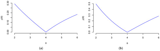
(Uniform Location Model). Set $\mathcal{Y}=(0,\infty )$ and $\mathsf{\Theta }=(0,\infty )$. Consider the uniform location model

$$f_{\theta }\left(y\right)={\theta }^{-1}1(0\le y\le \theta ).$$

The Hellinger distance is

$$\rho \left(\theta \right)=1-\frac{\left(\theta +{\theta }_o-|\theta -{\theta }_o|\right)}{2\sqrt{\theta {\theta }_o}}.$$

Since the unique solution to $\frac{1}{2\sqrt{\theta {\theta }_o}}\left(\theta +{\theta }_o-|\theta -{\theta }_o|\right)=1$ is $\theta ={\theta }_o$, see Figure 1a, one has $arg{min}_{\theta \in \mathsf{\Theta }}\rho \left(\theta \right)={\theta }_o$.

Figure 1. The Hellinger distance in Examples 1 and 2. (a) Example 1 (${\theta }_o=4$); (b) Example 2 (${\theta }_o=4$, $m=5$).

The Fisher matrix is $\mathcal{I}\left({\theta }_o\right)=0$, which is a singular matrix.

Example 2

(First-Price Auction Model). Consider the first-price procurement auction model with m bidders introduced in (Paarsch 1992, Section 4.2.2). For bidders with independent private valuations, following an exponential distribution with parameter θ (Paarsch 1992, Display 4.18) shows that the density of the wining bid $Y_i$ in the i-th auction is

$$f_{\theta }\left(y\right)=\frac{m}{\theta }exp\left(\frac{m}{m-1}-\frac{m}{\theta }y\right)1\left(y\ge \frac{\theta }{m-1}\right).$$

Set $\mathcal{Y}={\mathbb{R}}_{+}$ and $\mathsf{\Theta }=(0,\infty )$. The Hellinger distance in this case is

$$\rho \left(\theta \right)=1-\frac{2\sqrt{\theta {\theta }_o}}{(\theta +{\theta }_o)}exp{\left(1-\frac{(\theta +{\theta }_o)}{2\theta {\theta }_o}max(\theta ,{\theta }_o)\right)}^{\frac{m}{m-1}}.$$

For $\theta <{\theta }_o$ (resp. $\theta >{\theta }_o$), one has $▿\rho \left(\theta \right)<0$ ($▿\rho \left(\theta \right)>0$), see Figure 1b. Hence, by continuity of $\theta \mapsto \rho \left(\theta \right)$, $arg{min}_{\theta \in \mathsf{\Theta }}\rho \left(\theta \right)={\theta }_o$. The Fisher matrix is $\mathcal{I}\left({\theta }_o\right)=0$, which is a singular matrix.

Example 3

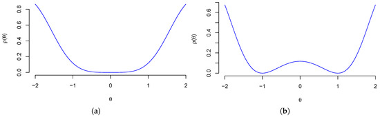
(Normal Squared Location Model). Set $\mathcal{Y}=\mathbb{R}$ and $\mathsf{\Theta }=\mathbb{R}$. Consider the normal squared location model

$$f_{\theta }\left(y\right)={\left(\sqrt{2\pi }\right)}^{-1}exp\left[-{(y-{\theta }^2)}^2/2\right].$$

This model would arise, for example, if Y is the difference between a matched pair of random variables whose control and treatment labels are not observed. The Hellinger distance is

$$\rho \left(\theta \right)=1-exp(-{({\theta }^2-{\theta }_o^2)}^2/8).$$

The parameter point ${\theta }_o=0$ is identifiable because $\theta \mapsto 1-exp(-{\theta }^4/8)$ is a strictly convex function, see Figure 2a. The parameter points ${\theta }_o\ne 0$ are not identifiable because $\rho \left({\theta }_o\right)=\rho (-{\theta }_o)=0$, see Figure 2b. The Fisher matrix is $\mathcal{I}\left({\theta }_o\right)=4{\theta }_o^2$, which implies that $\mathcal{I}\left(0\right)=0$ is a singular matrix and ${\theta }_o=0$ is an irregular point of the Fisher matrix.

Figure 2. The Hellinger distance in Example 3. (a) Example 3 (${\theta }_o=0$); (b) Example 3 (${\theta }_o=1$).

Example 4

(Demand-and-Supply Model). Let $Y=(P,Q)$ denote the observed price and quantity of a good transacted in a market at a given period of time. Linear approximations to the demand and supply functions are

$$\begin{array}{ccc}\hfill D& =\alpha +\beta P+V\hfill & \hfill \hspace{1em}\hspace{1em}\hspace{1em}\hspace{1em}\text{(Demand)}\\ \hfill S& =\gamma +\delta P+U\hfill & \hfill \hspace{1em}\hspace{1em}\hspace{1em}\hspace{1em}\text{(Supply)}\\ \hfill Q& =D=S,\hfill & \hfill \hspace{1em}\hspace{1em}\hspace{1em}\hspace{1em}\text{(Equilibrium)}\end{array}$$

where $\alpha ,\beta ,\gamma ,\delta$ are unknown parameters and $(U,V)$ is an unobserved random vector. Assume that U and V are independent and jointly normal distributed with mean zero and unknown variance ${\sigma }_{11}$ and ${\sigma }_{22}$, respectively. Set $\theta =(\alpha ,\beta ,\gamma ,\delta ,{\sigma }_{11},{\sigma }_{22})$. The density of the observed variables is then

$$f_{\theta }\left(y\right)=\frac{exp\left(-\frac{1}{2}{(y-\mu )}^{\prime }{\mathsf{\Omega }}^{-1}(y-\mu )\right)}{\sqrt{{\left(2\pi \right)}^{2}det\left(\mathsf{\Omega }\right)}},$$

where $det(·)$ is the determinant of the matrix in the parenthesis and

$$\begin{array}{c}\hfill \mu =\left(\begin{array}{c}\frac{\alpha -\gamma }{\delta -\beta }\\ \frac{\delta \alpha -\beta \gamma }{\delta -\beta }\end{array}\right) and \mathsf{\Omega }=\left(\begin{array}{cc}\frac{{\sigma }_{11}+{\sigma }_{22}}{{(\alpha -\gamma )}^2}& \frac{\delta {\sigma }_{11}+\beta {\sigma }_{22}}{{(\alpha -\gamma )}^2}\\ \frac{\delta {\sigma }_{11}+\beta {\sigma }_{22}}{{(\alpha -\gamma )}^2}& \frac{{\delta }^2{\sigma }_{11}+{\beta }^2{\sigma }_{22}}{{(\alpha -\gamma )}^2}\end{array}\right).\end{array}$$

The squared Hellinger distance is

$$\rho \left(\theta \right)=1-\frac{det{\left(\mathsf{\Omega }\right)}^{1/4}det{\left({\mathsf{\Omega }}_o\right)}^{1/4}}{det{\left(\frac{\mathsf{\Omega }+{\mathsf{\Omega }}_o}{2}\right)}^{1/2}}exp\left(-\frac{1}{8}{(\mu -{\mu }_o)}^{\prime }{\left(\frac{\mathsf{\Omega }+{\mathsf{\Omega }}_o}{2}\right)}^{-1}(\mu -{\mu }_o)\right).$$

To show that ${\theta }_o$ is not identifiable, by Proposition 1, it suffices to verify that $arg{min}_{\theta }\rho \left(\theta \right)$ is not a singleton. We elaborate on this point in the Supplementary Material.

Example 5

(Laplace Location Model). Set $\mathcal{Y}=\mathbb{R}$, $\mathsf{\Theta }=\mathbb{R}$. Consider the Laplace location model

$$f_{\theta }\left(y\right)=\frac{1}{2}exp(-|y-\theta \left|\right).$$

The squared Hellinger distance is

$$\rho \left(\theta \right)=1-exp\left(-\frac{|\theta -{\theta }_o|}{2}\right)-\frac{\delta }{2}\left[1(\theta -{\theta }_o>0)exp\left(-\frac{\theta -{\theta }_o}{2}\right)-1(\theta -{\theta }_o<0)exp\left(\frac{\theta -{\theta }_o}{2}\right)\right].$$

For any $\theta -{\theta }_o<0$ ($\theta -{\theta }_o<0$), one has $▿\rho \left(\theta \right)>0$ ($▿\rho \left(\theta \right)>0$). By continuity, $\theta \mapsto \rho \left(\theta \right)$ has then a unique minimizer at $\theta ={\theta }_o$, and, by Proposition 1, ${\theta }_o$ is identifiable. The Fisher matrix is $\mathcal{I}\left(\theta \right)=1$, which is a non-singular matrix.

Example 6

(Exponential Mixture). Set $\mathcal{Y}=[0,\infty ]$, $\theta ={({\theta }_1,{\theta }_2,{\theta }_3)}^{\prime }$ and $\mathsf{\Theta }=[0,1]\times [0,\infty )\times [0,\infty )$. Consider the finite mixture of exponential model

$$f_{\theta }\left(y\right)=(1-{\theta }_1)exp(ln{\theta }_2-{\theta }_{2}y)+{\theta }_{1}exp(ln{\theta }_3-{\theta }_{3}y).$$

Consider ${\theta }_o=(1/2,1,2)$ and ${\theta }_{★}=(1/2,2,1)$. Since $f_{{\theta }_o}^{1/2}=f_{{\theta }_{★}}^{1/2}$, one has $\rho \left({\theta }_{★}\right)=0$ and ${\theta }_{★}\in arg{min}_{\theta \in \mathsf{\Theta }}\rho \left(\theta \right)$. Since ${\theta }_o\ne {\theta }_{★}$, it follows from Proposition 1 that ${\theta }_o$ is not identifiable.

The previous examples also illustrate the difference between identifiable and local identifiable points in the parameter space.

Example 7

(Normal Squared Location Model, Continued). In this example, any ${\theta }_o\in \mathsf{\Theta }$ is locally identifiable—even the irregular point ${\theta }_o=0$ to the Fisher matrix—and only ${\theta }_o=0$ is identifiable, see Figure 2.

We also have the following criterion for local identifiability based on minimizing the squared Hellinger distance.

Proposition 2.

The parameter ${\theta }_o\in \mathsf{\Theta }$ is locally identifiable in the model ${\mathcal{F}}_{\mathsf{\Theta }}$ if and only if there exists an open set ${\mathsf{\Theta }}_{★}\ni {\theta }_o$ such that

$${\theta }_o=arg\underset{\theta \in {\mathsf{\Theta }}_{★}}{min}\rho \left(\theta \right).$$

This criterion, unlike the criterion based on the Fisher matrix by Rothenberg (1971) and re-stated below as Lemma 3 for the sake of completeness, applies to the case when:

• the support of Y depends on the parameter of interest;
• ${\theta }_o$ is not a regular point of the Fisher matrix;
• some elements of the Fisher matrix $\mathcal{I}\left({\theta }_o\right)$ are not defined;
• $\theta \mapsto \mathcal{I}\left(\theta \right)$ is not continuous;
• Θ is infinite-dimensional.

Proposition 2 reduces local identifiability to a unique solution of a well-defined minimization problem. One general criterion, and, as argued, e.g., (Rockafellar and Wets 1998), virtually the only available one, to check in advance for the uniqueness of a minimizer of an optimization problem is the strict convexity of the objective function. The application of this general criterion to the characterization of local identifiability in Proposition 2 yields the following result:

Proposition 3.

If $\theta \mapsto \rho \left(\theta \right)$ is a locally strictly convex function around ${\theta }_o$ (i.e., if there is an open convex set ${\mathsf{\Theta }}_{★}\ni {\theta }_o$ such that $\rho :{\mathsf{\Theta }}_{★}\mapsto [0,1]$ is a strictly convex function), then ${\theta }_o$ is locally identifiable.

Proposition 3 leads to the observation that local identifiability can be seen to be related to the local convexity of the Hellinger distance. As with our earlier propositions, it holds when the support of Y depends on the parameter of interest, ${\theta }_o$ is not a regular point of the Fisher matrix, some elements of the Fisher matrix $\mathcal{I}\left({\theta }_o\right)$ are not defined or $\theta \mapsto \mathcal{I}\left(\theta \right)$ is not continuous.

3. The Fisher Matrix Criterion

Rothenberg (1971) gives a criterion for local identifiability in terms of the non-singularity of the Fisher matrix. Additional insight about the relevance—and limitations—of the Fisher matrix criterion for local identifiability may then be gained by relating it to the criterion based on minimizing the Hellinger distance. To study this relationship, we now focus on the regular models studied by Rothenberg (1971).

Assumption 1

(R (Regular Models)). ${\mathcal{F}}_{\mathsf{\Theta }}$ is such that:

(A1) Θ is an open set in ${\mathbb{R}}^K$.

(A2) $f_{\theta }\ge 0$ and $\int f_{\theta }d\mu =1$ for all $\theta \in \mathsf{\Theta }$.

(A3) $supp\left(f_{\theta }\right):=\{y\in \mathcal{Y}:f_{\theta }\left(y\right)>0\}$ is the same for all $\theta \in \mathsf{\Theta }$.

(A4) For all θ in a convex set containing Θ and for all $y\in supp\left(f_{\theta }\right)$, the functions $\theta \mapsto f_{\theta }$ and $\theta \mapsto \ell \left(\theta \right):=ln{f}_{\theta }$ are continuously differentiable.

(A5) The elements of the matrix $\mathbb{E}[▿\ell \left(\theta \right)▿\ell {\left(\theta \right)}^{\top }]$ are finite and are continuous functions of θ everywhere in Θ.

We now replicate the characterization of local identifiability by Rothenberg (1971) Theorem 1 based on the non-singularity of the Fisher matrix.

Lemma 3.

Let the regularity conditions in Assumption R hold. Let ${\theta }_o$ be a regular point of the Fisher matrix $\mathcal{I}\left({\theta }_o\right)$. Then, ${\theta }_o$ is locally identifiable if and only if $\mathcal{I}\left({\theta }_o\right)$ is non-singular.

This characterization of local identifiability only applies to the regular models defined by Assumption R and to the regular points of the Fisher matrix, which may be a subset of the parameter space (see Example 3). These conditions do not have themselves any direct statistical or economic interpretation: their role is just to permit a characterization of local identifiability.3 We have already referenced in the introduction a list of models with irregular points of the Fisher matrix, for which the characterization in Lemma 3 does not apply. We now use Examples 1–5 to illustrate the notions of regular and irregular models and their implications for the analysis of identifiability. The richness of the possibilities that follow is a recall of the care needed in using the Fisher matrix criterion for showing local identifiability (or lack of it). It also highlights the convenience of the identifiability criterion based on minimizing the Hellinger distance as a unifying approach to study the identifiability of regular or irregular points of the Fisher matrix in either regular or irregular models. Specifically:

• The uniform location model in Example 1 and the first-price auction model in Example 2 have, respectively, $supp\left(f_{\theta }\right)=[0,1/\theta ]$ and $supp\left(f_{\theta }\right)=[\theta /[m-1],\infty )$, which means that these models violate the regularity condition $\left(A3\right)$. We have seen that ${\theta }_o$ is identifiable in Examples 1 and 2, which implies that $\left(A3\right)$ is not necessary for identifiability. These models also have a singular Fisher matrix, which implies that, in irregular models violating $\left(A3\right)$, the non-singularity of the Fisher matrix is not a necessary condition for (local) identifiability.
• One can verify that the normal squared location model in Example 3 and the normal supply-and-demand model in Example 4 both satisfy the regularity conditions in Assumption R. We have seen that in Example 3 the parameter of interest is locally identifiable while in Example 4 it is not, which means that the regularity conditions in Assumption R are not sufficient or necessary for (local) identifiability, they are just convenient. In Example 3, moreover, ${\theta }_o=0$ is not a regular point of the Fisher matrix and is locally identifiable, which implies that, for irregular points of the Fisher matrix, the non-singularity of the Fisher matrix is not a necessary condition for (local) identifiability.
• In Example 5, the function $\theta \mapsto ln(1/2)-|y-\theta |$ is not differentiable when $y=\theta$, which means that the Laplace location model is an irregular model because it violates $\left(A4\right)$.
• To illustrate a failure of $\left(A1\right)$ and $\left(A5\right)$, consider the finite mixture of exponential model in Example 6 with ${\theta }_1=0$, ${\theta }_2=1$ and ${\theta }_3=0.5$. In this case, $\mathbb{E}[▿\ell \left(0\right)▿\ell {\left(0\right)}^{\top }]={(1-2)}^2/\left[2(2-2)\right]$, which is not finite.

We also have the following result linking the Hellinger distance to the Fisher matrix, which we are going to use to show that, in regular models with irregular points to the Fisher matrix, the non-singularity of the Fisher matrix is only a sufficient condition for local identifiability.

Lemma 4.

Let the regularity conditions in Assumption R hold and assume that $\theta \mapsto \ell \left(\theta \right):=f_{\theta }^{1/2}$ is continuously differentiable μ-a.e. Then, the Hellinger distance and the Fisher matrix are related by

$${▿}^2\rho \left({\theta }_o\right)=c\mathcal{I}\left({\theta }_o\right),where c=1/4.$$

Though this result is known, see, e.g., (Borovkov 1998), its implications for local identifiability have so far not been drawn.

Since the Fisher matrix is a variance-covariance matrix, one has that $\mathcal{I}\left(\theta \right)$ is, under $\left(A5\right)$, a real symmetric semi-definite positive matrix for every $\theta \in \mathsf{\Theta }$, and then the following result follows from Lemma 4 and the characterization of a convex function in terms of its Hessian, see, e.g., (Rockafellar and Wets 1998, Theorem 2.14).

Proposition 4.

Let the regularity conditions in Assumption R hold and assume that $\theta \mapsto f_{\theta }^{1/2}$ is continuously differentiable μ-a.e. Then, $\theta \mapsto \rho \left(\theta \right)$ is a locally convex function around ${\theta }_o$. Furthermore, if $\mathcal{I}\left({\theta }_o\right)$ is non-singular, then $\theta \mapsto \rho \left(\theta \right)$ is a locally strict convex function around ${\theta }_o$ and ${\theta }_o$ is locally identifiable.

Two remarks are in order. First, notice that, unlike Lemma 3, the result in Proposition 4 also applies when ${\theta }_o$ is not a regular point of the Fisher matrix and the non-singularity of the Fisher matrix becomes only sufficient for local identifiability. Second, if $\mathcal{I}\left({\theta }_o\right)$ is singular, the function $\rho :{\mathsf{\Theta }}_{★}\to [0,1]$ is still locally convex (because $\mathcal{I}\left({\theta }_o\right)$ is positive semi-definite) and $arg{min}_{\theta \in {\mathsf{\Theta }}_{★}}\rho \left(\theta \right)$ is a convex, but not necessarily bounded, set, which is a result that can be used to delineate the set of observational equivalent values of ${\theta }_o$. This note does not pursue this interesting direction.

Table 1 summarizes the information in this note about the necessity and sufficiency of the non-singularity of the Fisher matrix for local identifiability.

Table 1. For local identifiability, the non-singularity of the Fisher Matrix is ....

	Regular Points	Irregular Points
Regular Models	necessary and sufficient (Lemma 3)	only sufficient (Proposition 4 and Example 3)
Irregular Models	not necessary (Examples 1, 2, and 5)

We conclude this section by mentioning that, in response to the misbehavior of the Fisher matrix when informing about the difficulty to estimate parameters of interest in parametric models, alternative notions of information, other than the Fisher matrix, have been proposed in the literature (see, e.g., Donoho and Liu 1987). Without further elaboration, these alternative notions of information are not directly applicable to construct new criteria of identifiability. In particular, the geometric information based on the modulus of continuity of ${\theta }_o\mapsto arg{min}_{\theta }\rho \left(\theta \right)$ with respect to the Hellinger distance, introduced by Donoho and Liu (1987) to geometrize convergence rates, cannot be used to construct a criterion for local identifiability because this modulus of continuity, in its current format, is not defined for parameters that are not locally identifiable.4

4. The Kullback–Liebler Divergence and Other Divergences

Some of the examples where we have had success in using the Hellinger distance to analyze identifiability share the same structure: the Hellinger distance is a locally convex function, see Figure 2, and so the results from convex optimization become available. If the Hellinger distance proves to be difficult to analyze, one can set out a criterion for identifiability based on another divergence function, such as the reversed Kullback–Liebler divergence (see, e.g., Bowden 1973)

$$\kappa \left(\theta \right)=-H\left(\theta \right),\mathrm{where}H\left(\theta \right):=\int ln\left(\frac{f_{\theta }}{f_{{\theta }_o}}\right)f_{{\theta }_o}d\mu .$$

One can unify the identification criteria based on the Hellinger distance and the reversed Kullback–Liebler divergence by using the family of $\phi$-divergences defined as

$${\delta }_{\phi }\left(\theta \right)=\int \phi \left(\frac{f_{\theta }}{f_{{\theta }_o}}\right)d\mu ,$$

where $f_{\theta }/f_{{\theta }_o}$ is the likelihood ratio and $\phi :\mathbb{R}\to [0,+\infty ]$ is a proper closed convex function with $\phi \left(1\right)=0$ and such that $x\mapsto \phi \left(x\right)$ is strictly convex on a neighborhood of $x=1$. The squared Hellinger distance corresponds to the member of this family with $\phi \left(x\right)=\frac{1}{2}{(1-\sqrt{x})}^2$, whereas the reversed Kullback–Liebler divergence corresponds to $\phi \left(x\right)=-lnx+x-1$. The following result is an immediate consequence of the property that ${\delta }_{\phi }$ is non-negative and it is equal to zero if and only if $f_{\theta }=f_{{\theta }_o}$ (see, e.g., Pardo 2005, Proposition 1.1)).

Proposition 5.

The parameter ${\theta }_o\in \mathsf{\Theta }$ is locally identifiable in the model ${\mathcal{F}}_{\mathsf{\Theta }}$ if and only if there exists an open set ${\mathsf{\Theta }}_{★}\ni {\theta }_o$ such that

$${\theta }_o=arg\underset{\theta \in {\mathsf{\Theta }}_{★}}{min}{\delta }_{\phi }\left(\theta \right).$$

This result, which is a generalization of Proposition 2, shows that the choice of a $\phi$-divergence for analyzing the identifiability of a parameter of interest only hinges on the difficulty to characterize the set $arg{min}_{\theta }{\delta }_{\phi }\left(\theta \right)$ for a given $\phi$-divergence. The choice of the Hellinger distance over the reversed Kullback–Liebler divergence is, however, not inconsequential when choosing $\phi$-divergence to construct an estimator for the parameter of interest. The use of the Hellinger distance may lead to an estimator that is more robust than the maximum likelihood estimator and equally efficient, see, e.g., Beran (1977) and Jimenez and Shao (2002).5

We conclude this section with the following result showing that, for the regular models analyzed by Rothenberg (1971), the Hellinger distance and the reversed Kullback–Liebler divergence are both locally convex around a minimizer.

Lemma 5.

Let the regularity conditions in Assumption R hold and assume that $\theta \mapsto f_{\theta }^{1/2}$ is continuously differentiable μ-a.e. Let us assume, furthermore, that, in a neighborhood of ${\theta }_o$, $f_{\theta }$ and $ln{f}_{\theta }$ are twice differentiable in θ, with derivatives continuous in $y\in supp\left(f_{\theta }\right)$. Then, the Hellinger distance and the Kullback–Liebler divergence are related by

$${▿}^2\rho \left({\theta }_o\right)=c{▿}^2\kappa \left({\theta }_o\right)forc=1/4.$$

References

- Beran, R. 1977. Minimum Hellinger Distance Estimates for Parametric Models. The Annals of Statistics 5: 445–63. [Google Scholar] [CrossRef]
- Borovkov, A. 1998. Mathematical Statistics. Amsterdam: Gordon and Breach. [Google Scholar]
- Bowden, R. 1973. The Theory of Parametric Identification. Econometrica 41: 1069. [Google Scholar] [CrossRef]
- Donoho, D., and R. Liu. 1987. Geometrizing Rates of Convergence, I. Technical Report 137. Berkeley: University of California. [Google Scholar]
- Escanciano, J. C. 2021. Semiparametric Identification and Fisher Information. Econometric Theory, 1–38. [Google Scholar]
- Hallin, M., and C. Ley. 2012. Skew-Symmetric Distributions and Fisher Information—A Tale of Two Densities. Bernoulli 18: 747–63. [Google Scholar] [CrossRef]
- Han, S., and A. McCloskey. 2019. Estimation and Inference with a (Nearly) Singular Jacobian. Quantitative Economics 10: 1019–68. [Google Scholar] [CrossRef]
- Hinkley, D. 1973. Two-Sample Tests with Unordered Pairs. Journal of the Royal Statistical Association (Series B: Methodological) 36: 2466–80. [Google Scholar] [CrossRef]
- Jimenez, R., and Y. Shao. 2002. On Robustness and Efficiency of Minimum Divergence Estimators. Test 10: 241–48. [Google Scholar] [CrossRef]
- Lee, L., and A. Chesher. 1986. Specification Testing when Score Test Statistics are Identically Zero. Journal of Econometrics 31: 121–49. [Google Scholar] [CrossRef]
- Lewbel, A. 2019. The Identification Zoo: Meanings of Identification in Econometrics. Journal of Economic Literature 57: 835–903. [Google Scholar] [CrossRef]
- Li, P., J. Chen, and P. Marriot. 2009. Non-Finite Fisher Information and Homogeneity: And EM Approach. Biometrika 96: 411–26. [Google Scholar] [CrossRef]
- Paarsch, H. 1992. Deciding between the Common and Private Value Paradigms in Empirical Models of Auctions. Journal of Econometrics 51: 191–215. [Google Scholar] [CrossRef]
- Pardo, L. 2005. Statistical Inference Based on Divergence Measures. New York: Chapman & Hall/CRC Press. [Google Scholar]
- Paulino, C., and C. Pereira. 1994. On Identifiability of Parametric Statistical Models. Journal Italian Statistical Society 3: 125–51. [Google Scholar] [CrossRef]
- Reiersol, O. 1950. The Identifiability of a Linear Reation between Variables which are Subject to Error. Econometrica 18: 375–89. [Google Scholar] [CrossRef]
- Rockafellar, T., and R. Wets. 1998. Variational Analysis. Berlin: Springer. [Google Scholar]
- Rothenberg, R. 1971. Identification in Parametric Models. Econometrica 39: 577–91. [Google Scholar] [CrossRef]
- Sargan, J. 1983. Identification and Lack of Identification. Econometrica 51: 1605–33. [Google Scholar] [CrossRef]
Publisher’s Note: MDPI stays neutral with regard to jurisdictional claims in published maps and institutional affiliations. |
© 2022 by the author. Licensee MDPI, Basel, Switzerland. This article is an open access article distributed under the terms and conditions of the Creative Commons Attribution (CC BY) license (https://creativecommons.org/licenses/by/4.0/).