Detecting Location Shifts during Model Selection by Step-Indicator Saturation

Abstract

To capture location shifts in the context of model selection, we propose selecting significant step indicators from a saturating set added to the union of all of the candidate variables. The null retention frequency and approximate non-centrality of a selection test are derived using a ‘split-half’ analysis, the simplest specialization of a multiple-path block-search algorithm. Monte Carlo simulations, extended to sequential reduction, confirm the accuracy of nominal significance levels under the null and show retentions when location shifts occur, improving the non-null retention frequency compared to the corresponding impulse-indicator saturation (IIS)-based method and the lasso.

1. Introduction

Unmodelled location shifts (changes in previous unconditional means of data) can have pernicious effects on the constancy of models and on forecast performance. In sample, an unmodelled location shift entails that empirical models will be misspecified, potentially affecting which variables, their lags and non-linear functions will be selected, distorting parameter estimation and inference, as well as inducing non-constancy: see [1]. Out of sample, an unanticipated location shift at or near the forecast origin can lead to forecast failure: see [2]. Consequently, we consider step-indicator saturation (SIS) to detect location shifts as part of a model selection strategy, building on the developments of impulse-indicator saturation (IIS). Hendry et al. [3] derive the null distribution of IIS for independent, identically distributed ($\mathsf{IID}$) data, and [4] generalize that analysis to dynamic regression models (possibly with unit roots). Hendry and Santos [5] propose an IIS-based test of super exogeneity, building on [6]; and [7,8,9,10,11,12] provide empirical applications of IIS.

Indicator saturation methods (such as IIS and SIS) are feasible because software, like Autometrics, can handle more candidate variables N than observations T during model selection using a combination of expanding and contracting multiple block searches, as described in [13],[14] (Chapter 19), and [15]. In this selection context, the null retention frequency of indicators is called the gauge by [16], akin to the size of a test denoting its (false) null rejection frequency, but taking into account that indicators that are insignificant on a pre-assigned criterion may nevertheless be retained to offset what would otherwise be a significant misspecification test. Johansen and Nielsen [4] establish that using small nominal significance levels α (e.g., $\alpha \le 0.01$) for selection in IIS, despite testing T indicators, on average, $\alpha T$ are retained, so the gauge is approximately α: also, see [17] for a discussion of outlier detection algorithms. The non-null retention frequency when selecting indicators is called its potency, akin to a similar test’s power for rejecting a false null hypothesis: see [10] for simulations of IIS under the alternative. The analytic derivations below use the split-half one-cut approach in [3] for establishing the distribution under the null of no shifts, checked by simulations that also compare split-half sequential selection outcomes and a multi-path search algorithm, extended to non-null alternatives.

When the locations, durations, magnitudes and signs of multiple shifts are unknown, we show that selection by SIS can be beneficial. There are many extant tests for multiple breaks, such as those proposed by [18,19,20]. Our interest is in joint selection over candidate variables, dynamic reactions and possible non-linearities, investigated in detail by [14], and since location shifts can approximate non-linearities and vice versa (see, e.g., [21]), we do not explore the pre-testing route. Importantly, SIS does not require knowledge of the locations of breaks, the maximum number of shifts, nor does it impose a minimum break length, so it allows shifts to occur at the start and/or end of the sample. Alternative model selection methods include the lasso and least angle regression, as described by [22,23] respectively. lasso and least angle regression (LARS) work well for a single step shift, but once multiple breaks occur, because of the forward selection approach they adopt, selection over multiple step functions can fail to detect shifts, as no single step function is highly correlated with any of the multiple breaks.

The structure of this paper is as follows. Section 2 describes step-indicator saturation, then Section 3 derives its gauge in a split-half one-cut analysis. Monte Carlo experiments are reported following each theory section, so the gauge of SIS is simulated in Subsection 3. The numerical results are based on simulating in Ox and Autometrics: see [24,25]. Section 4 investigates the power of a step indicator to detect a known mean shift and relates that to well-known procedures, such as the test of [26]. We next consider selecting indicators for unknown shifts in Section 5, first Subsection 5.1, which develops the basic analytical tools, and is simulated in Subsection 5.2. Subsection 5.3 considers the effects of misspecifying the timing of an indicator. The basic setting is generalized in Subsection 5.4 to unknown shifts requiring a two-step (off-on-off) indicator; two opposite-signed shifts where one lies in each half in Subsection 5.5, with the same-signed shifts in each half in Subsection 5.6; then, to an unknown shift spanning both splits in Subsection 5.7, with a summary of the simulation results in Subsection 5.8. A generalization to retained regressors is noted in Section 6. Section 7 provides comparisons with LARS, and Section 8 investigates the impact on selecting non-linearity when SIS is applied. Section 9 concludes.

2. Step-Indicator Saturation

Consider adding a complete set of step indicators, ${\mathcal{S}}_1=\left\{1_{\left\{t\le j\right\}},j=1,\dots ,T\right\}$, to a regression model, where $1_{\left\{t\le j\right\}}=1$ for observations up to j, and zero otherwise. Step indicators are the cumulation of impulse indicators up to each next observation. As whole-sample vectors, step indicators take the form ${\iota }_1^{\prime }=($1,0,0,…,0), ${\iota }_2^{\prime }=($1,1,0,…,0), …, ${\iota }_T^{\prime }=($1,1,1,…,1), which is the intercept dummy. As in [27], n valid conditioning variables ${\mathbf{z}}_t$ can be retained without selection for $n<T/2$. Under the null of no shifts, the initial specification is:

$$y_t={\beta }_0+{\beta }_1^{\prime }{\mathbf{z}}_t+u_t\text{where}{u}_t\sim \mathsf{IN}\left[0,{\sigma }_u^2\right]$$

(1)

when $\mathsf{IN}\left[0,{\sigma }_u^2\right]$ denotes an independent normal distribution with mean zero and variance ${\sigma }_u^2$. Adding the saturating set of step indicators ${\mathcal{S}}_1$ to Equation (1) creates:

$$y_t={\beta }_0+{\beta }_1^{\prime }{\mathbf{z}}_t+\sum _{j=1}^{T-1}{\delta }_j{1}_{\left\{t\le j\right\}}+u_t$$

(2)

It is infeasible to estimate (2), but the split-half one-cut approach to understanding IIS applies to SIS. First consider $n=0$. Add the first $k=T/2$ indicators to Equation (1) and record which have significant coefficients at significance level α. As $k<T$ and the indicators are deterministic, conventional inference applies. Drop the first half and add the second block of $T/2$ to the original model (1), again recording which are significant in that subset. Finally, combine the recorded variables (if any) from the two stages, and select again at significance level α. Under the null, setting $\alpha =1/T$, on average, at both sub-steps, $\alpha T/2$ (namely $1/2$ an indicator) will be retained by chance, so on average, $\alpha T=1$ indicator will be retained from the combined stage, so one degree of freedom is lost on average. Hendry et al. [3] show that other splits, such as using r splits of size $T/r$, or unequal splits, do not affect the gauge, or simulation-based distributions. When $n\ne 0$ and $n+k>T$, divide the total set of $N=n+T$ candidate variables into smaller sub-blocks, setting $\alpha =1/N$ overall.

When m indicators are selected in a congruent representation at significance level α:

$$y_t={\beta }_0+{\beta }_1^{\prime }{\mathbf{z}}_t+\sum _{i=1}^m{\varphi }_{i,\alpha }{1}_{\left\{t\le T_i\right\}}+v_t\text{where}{v}_t\sim \mathsf{IN}\left[0,{\sigma }_v^2\right]$$

(3)

and the coefficients of significant indicators are denoted ${\varphi }_{i,\alpha }$. Despite some similarities between the procedures in IIS and SIS, there are important differences necessitating a new analysis. First, while impulse indicators are mutually orthogonal, step indicators overlap increasingly as their second index increases. Second, for an impulse, or more generally, a location shift that is not at either end, say from $T_1$ to $T_2$, two indicators are required to characterize it: $1_{\left\{t\le T_2\right\}}-1_{\left\{t<T_1\right\}}$. Third, the ease of detection may be affected by whether location shifts occur with similar, or opposite, signs and magnitudes. Although we use a split-half one-cut approach for analysis, in practice, the combination of expanding and contracting multiple block searches as implemented in Autometrics should be applied. Bergamelli and Urga [28] undertake extensive simulations of IIS, SIS and their extensions to trend breaks, as well as comparisons with the sequential break tests in [29] and, using different block partitions, find similar results to those reported below.

There are many possible specifications of step indicators, but the choice should have little impact on the detection of location shifts, corroborated by simulation comparisons. More generally, the shape of shift indicators can be specified in light of subject-matter considerations. For example, to detect the impact of volcanic eruptions on tree-ring measures of temperature, [30] designed a ν-shaped formulation that proved successful; an ogive shape could represent a slower step shift as in the logistic smooth-transition approach of [31]; or a neural network: see, e.g., [32].1

3. Null Retention Frequency (Gauge) of Step-Indicator Selection

To investigate the gauge of SIS, we consider the simplest constant-parameter data generation process (DGP):

$$y_t=\mu +{ϵ}_t\text{where}{ϵ}_t\sim \mathsf{IN}\left[0,{\sigma }_{ϵ}^2\right]$$

(4)

As with IIS, we use the split-half one-cut approach under the null, so there are $T/2$ indicators for the first half:

$$y_t=\mu +\sum _{j=1}^{T/2}{\delta }_j{1}_{\left\{t\le j\right\}}+u_t$$

(5)

the equation of which can be estimated directly, indicators being retained when their estimated coefficients ${\widehat{\delta }}_j$ satisfy $|{\mathsf{t}}_{{\widehat{\delta }}_j}|>c_{\alpha }$, where $c_{\alpha }$ is the critical value for significance level α. Under the null, a subset $\alpha T/2$ of the indicators will be retained by chance on average. Their locations are recorded; all of those indicators are dropped, and the second set is then investigated in a similar way, now including indicators $1_{\left\{t\le j\right\}}$ for $j=T/2+1,\dots ,T-1$. Add the step indicators selected in each half to Equation (4), and re-select, keeping only significant indicators: an F-test of their joint significance could be conducted.

Figure 1 illustrates the split-half one-cut approach to SIS for Equation (4) when $\mu =10$, ${\sigma }_{ϵ}^2=1$ and $T=100$. The three rows correspond to the three stages: add the first half of the indicators, the second half, then the selected indicators combined. The three columns report the indicators entered, the indicators retained and the fitted and actual values of the selected model. Fifty indicators are added, and two are retained in Row 1. When the second half is entered (Row 2), none is retained. Selecting over the two retained indicators again retains them. Different and multiple splits or unequal divisions entered into Equation (4) should not affect the retention probability under the null: a step shift should only be retained when it is present, here by chance due to a collection of sufficient magnitude, same-signed $\left\{{ϵ}_t\right\}$ over a sub-sample. In practice, multiple block searches, as in Autometrics, will be needed, as the null may be false.

Figure 1. Illustrating split-half one-cut step-indicator saturation (SIS) under the null of no shift in Equation (4).

Figure 1. Illustrating split-half one-cut step-indicator saturation (SIS) under the null of no shift in Equation (4).

When n is small, adding strongly exogenous regressors to the baseline Equation (4) as in Equation (1) will still allow unrestricted estimation of each half, so the above analysis is unaffected.

Non-normal, but continuous symmetric distributions $\mathsf{f}(·)$, with at least eight finite moments, entail using the appropriate critical value $c_{\alpha }$, where $\alpha =1-{\int }_{-c_{\alpha }/2}^{c_{\alpha }/2}\mathsf{f}\left(u\right)\text{d}u$. If conventional critical values are used for selection, [10] show that, e.g., IIS will retain indicators corresponding to what are judged ‘outliers’ relative to the normal when the error distribution is fat-tailed, and we anticipate that SIS will do likewise.

Retention of Step Indicators Under the Null Hypothesis of No Shift

We investigated the properties of SIS using simulations coded in the Ox programming language and replicated $M=$ 1,000 times. First, the model in (4) is estimated using the split-half one-cut approach where $\mu =0$, ${ϵ}_t\sim \mathsf{IN}[0,{\sigma }_{ϵ}^2]$ and ${\sigma }_{ϵ}^2=1$, for a sample size $T=100$ and various values of α. Table 1 records the retention frequency of irrelevant indicators (gauge) overall, as well as for the first $T/2$ ($D_1$) and second $T/2$ sets of indicators ($D_2$). The overall retention frequency of irrelevant indicators is close to α, so on average, $\alpha T$ irrelevant step indicators are retained under the null that no shifts occur.

Table 1. Proportion of irrelevant retained indicators under the null of no shift.

	Gauge
α	Overall	$D_1$	$D_2$
0.001	0.0018	0.0018	0.0018
0.01	0.013	0.013	0.013
0.05	0.056	0.057	0.054

Table 1. Proportion of irrelevant retained indicators under the null of no shift.

	Gauge
α	Overall	$D_1$	$D_2$
0.001	0.0018	0.0018	0.0018
0.01	0.013	0.013	0.013
0.05	0.056	0.057	0.054

4. Analytical Power of a Step-Indicator Test for a Known Mean Shift

We next investigate the power of a step indicator to detect a known mean shift from ${\lambda }_1\ne 0$ to ${\lambda }_1=0$ at time $0<T_1<T/2$ in the DGP:

$$y_t=\mu +{\lambda }_1{1}_{\left\{t\le T_1\right\}}+{ϵ}_t\text{where}{ϵ}_t\sim \mathsf{IN}\left[0,{\sigma }_{ϵ}^2\right]$$

(6)

where ${\lambda }_1\ne 0$, so the shift is from $\mu +{\lambda }_1$ to μ. To determine the power of a step-indicator test to detect the shift in Equation (6), the nesting model when the shift is known is:

$$y_t=\phi +{\delta }_{T_1}{1}_{\left\{t\le T_1\right\}}+v_t$$

(7)

Theorem 1. Let ${\psi }_{{\lambda }_1}^{*}=\sqrt{T^{*}}{\lambda }_1/{\sigma }_{ϵ}$ be the non-centrality of the t-test of ${\mathsf{H}}_0$:${\delta }_{T_1}=0$ in Equation (7) for the DGP in Equation (6) where $T^{*}=T_1(T-T_1)/T$, then:

$${\mathsf{t}}_{{\widehat{\delta }}_{T_1}}=\frac{\sqrt{T^{*}}{\widehat{\delta }}_{T_1}}{{\widehat{\sigma }}_{ϵ}}\approx \frac{\sqrt{T^{*}}({\widehat{\delta }}_{T_1}-{\lambda }_1)}{{\sigma }_{ϵ}}+\frac{\sqrt{T^{*}}{\lambda }_1}{{\sigma }_{ϵ}}\sim \mathsf{N}\left[{\psi }_{{\lambda }_1}^{*},1\right]$$

(8)

Proof. As ${\sum }_{t=1}^T{1}_{\left\{t\le T_1\right\}}={\sum }_{t=1}^{T_1}{1}_{\left\{t\le T_1\right\}}=T_1$, estimating (7) delivers:

$$\begin{array}{cc}\hfill \left(\begin{array}{c}\widehat{\phi }-\mu \\ {\widehat{\delta }}_{T_1}-{\lambda }_1\end{array}\right)& ={\left(\begin{array}{cc}T& T_1\\ T_1& T_1\end{array}\right)}^{-1}\left(\begin{array}{c}\sum _{t=1}^T{ϵ}_t\\ \sum _{t=1}^{T_1}{ϵ}_t\end{array}\right)=\left(\begin{array}{c}{\overline{ϵ}}_{\left(2\right)}\\ {\overline{ϵ}}_{\left(1\right)}-{\overline{ϵ}}_{\left(2\right)}\end{array}\right)\hfill \end{array}$$

where ${\overline{ϵ}}_{\left(1\right)}=T_1^{-1}{\sum }_{t=1}^{T_1}{ϵ}_t$, etc., and:

$$\mathsf{V}\left[\left(\begin{array}{c}\widehat{\phi }-\mu \\ {\widehat{\delta }}_{T_1}-{\lambda }_1\end{array}\right)\right]={\sigma }_{ϵ}^2{\left(T-T_1\right)}^{-1}\left(\begin{array}{cc}1& -1\\ -1& T_1^{-1}\left(T-T_1\right)+1\end{array}\right).$$

For the DGP in Equation (6):

$$\sqrt{T^{*}}\left({\widehat{\delta }}_{T_1}-{\lambda }_1\right)\sim \mathsf{N}\left[0,{\sigma }_{ϵ}^2\right]$$

(9)

Hence, neglecting the estimation uncertainty in ${\widehat{\sigma }}_{ϵ}^2$:

$${\mathsf{t}}_{{\widehat{\delta }}_{T_1}}=\frac{\sqrt{T^{*}}{\widehat{\delta }}_{T_1}}{{\widehat{\sigma }}_{ϵ}}\approx \frac{\sqrt{T^{*}}({\widehat{\delta }}_{T_1}-{\lambda }_1)}{{\sigma }_{ϵ}}+\frac{\sqrt{T^{*}}{\lambda }_1}{{\sigma }_{ϵ}}\sim \mathsf{N}\left[{\psi }_{{\lambda }_1}^{*},1\right]$$

(10)

where $T^{*}=T_1$ when there is no intercept. ☐

Then, ${\psi }_{{\lambda }_1}^{*}$ in Equation (10) is $\sqrt{T^{*}}$ times the corresponding non-centrality for an individual impulse indicator in [5], so ${\mathsf{t}}_{{\widehat{\delta }}_{T_1}}$ will have considerable power when ${\lambda }_1\ne 0$.

5. Potency of SIS for an Unknown Location Shift

We now develop the basic analytical tools for a shift that can be matched by a single step indicator in Subsection 5.1 and check the outcomes by simulation in Subsection 5.2. Subsection 5.3 considers the effects of misspecifying the timing of an indicator. The basic setting is generalized in Subsection 5.4 to an unknown shift period requiring a two-step indicator. Subsection 5.5 and Subsection 5.6 consider the occurrence of two shifts where one lies in each half, first when opposite-signed, then when they are equal magnitudes, signs and durations. Subsection 5.7 then considers an unknown shift spanning both halves where multi-path search across several splits is likely to outperform split-half one-cut; see [33] for more detailed simulation evidence and comparisons with IIS.

5.1. Unknown Shift Period Matched by a Single Step Indicator

We first show that detection of a single location shift falling entirely within a half-sample of the data ($0<T_1<T/2$) as in Equation (6) is feasible using the split-half one-cut analysis of step-indicator saturation. In matrix notation, let ${\iota }_{T_1}$ denote a $T\times 1$ vector with elements of unity till $T_1$ and zeroes thereafter, so the DGP is:

$$\mathbf{y}={\lambda }_1{\iota }_{T_1}+ϵ$$

(11)

As before, add the first half of the step indicators, assuming T is even, so the model becomes:

$$y_t=\sum _{j=1}^{T/2}{\gamma }_j{1}_{\left\{t\le j\right\}}+v_t$$

(12)

We assume an intercept of zero in Equation (12) to highlight the main aspects of the algebra, written in matrix form as:

$$\mathbf{y}={\mathbf{D}}_1{\gamma }_{\left(1\right)}+\mathbf{v}$$

(13)

where ${\gamma }_{\left(1\right)}={({\gamma }_1\dots {\gamma }_{T/2})}^{\prime }$ and ${\mathbf{D}}_1=({\iota }_1\dots {\iota }_{T/2})$.

Theorem 2. The distribution of the least-squares estimator of ${\gamma }_{\left(1\right)}$ in Equation (13) is:

$${\left({\widehat{\gamma }}_{\left(1\right)}-{\lambda }_1\mathbf{r}\right)}_{\widetilde{app}}\mathsf{N}\left[\mathbf{0},{\sigma }_{ϵ}^2{\left({\mathbf{D}}_1^{\prime }{\mathbf{D}}_1\right)}^{-1}\right]$$

(14)

where r is a $T/2\times 1$ vector with unity in the $T_1$-th position, and zeroes elsewhere.

Proof. From Equation (11):

$${\widehat{\gamma }}_{\left(1\right)}={\left({\mathbf{D}}_1^{\prime }{\mathbf{D}}_1\right)}^{-1}{\mathbf{D}}_1^{\prime }\mathbf{y}={\lambda }_1{\left({\mathbf{D}}_1^{\prime }{\mathbf{D}}_1\right)}^{-1}{\mathbf{D}}_1^{\prime }{\iota }_{T_1}+{\left({\mathbf{D}}_1^{\prime }{\mathbf{D}}_1\right)}^{-1}{\mathbf{D}}_1^{\prime }ϵ$$

(15)

where $\left({\mathbf{D}}_1^{\prime }{\mathbf{D}}_1\right)$ is:

$$\left(\begin{array}{c}{\iota }_1^{\prime }\\ {\iota }_2^{\prime }\\ ⋮\\ {\iota }_{T/2-1}^{\prime }\\ {\iota }_{T/2}^{\prime }\end{array}\right)({\iota }_1{\iota }_2\dots {\iota }_{T/2-1}{\iota }_{T/2})=\left(\begin{array}{cccccc}1& 1& 1& \dots & 1& 1\\ 1& 2& 2& \dots & 2& 2\\ 1& 2& 3& \dots & 3& 3\\ ⋮& ⋮& ⋮& \ddots & \ddots & ⋮\\ 1& 2& 3& \dots & T/2-1& T/2-1\\ 1& 2& 3& \dots & T/2-1& T/2\end{array}\right)$$

(16)

The inverse of $\left({\mathbf{D}}_1^{\prime }{\mathbf{D}}_1\right)$ is the ‘double difference’ matrix:

$${\left({\mathbf{D}}_1^{\prime }{\mathbf{D}}_1\right)}^{-1}=\left(\begin{array}{cccccc}2& -1& 0& \dots & 0& 0\\ -1& 2& -1& \dots & 0& 0\\ 0& -1& 2& \dots & 0& 0\\ ⋮& \ddots & \ddots & \ddots & \ddots & ⋮\\ 0& 0& 0& \dots & 2& -1\\ 0& 0& 0& \dots & -1& 1\end{array}\right)$$

(17)

Therefore:

$${\left({\mathbf{D}}_1^{\prime }{\mathbf{D}}_1\right)}^{-1}{\mathbf{D}}_1^{\prime }=\left(\begin{array}{cccccc}1& -1& 0& \dots & 0& 0\\ 0& 1& -1& \dots & 0& 0\\ 0& 0& 1& \dots & 0& 0\\ ⋮& ⋮& ⋮& \ddots & \ddots & ⋮\\ 0& 0& 0& \dots & 1& -1\\ 0& 0& 0& \dots & 0& 1\end{array}\right)$$

which is the forward-difference matrix. Consequently, letting $\nabla {ϵ}_t={ϵ}_t-{ϵ}_{t+1}$, from Equation (15):

$${\widehat{\gamma }}_{\left(1\right)}={\lambda }_1{\left({\mathbf{D}}_1^{\prime }{\mathbf{D}}_1\right)}^{-1}{\mathbf{D}}_1^{\prime }{\iota }_{T_1}+{\left({\mathbf{D}}_1^{\prime }{\mathbf{D}}_1\right)}^{-1}{\mathbf{D}}_1^{\prime }ϵ={\lambda }_1\mathbf{r}+\nabla {ϵ}_{\left(1\right)}$$

where r is a $T/2\times 1$ vector with unity in the $T_1$-th position and zeroes elsewhere, so:

$$\left({\widehat{\gamma }}_{\left(1\right)}-{\lambda }_1\mathbf{r}\right)=\nabla {ϵ}_{\left(1\right)}$$

(18)

where the ($T/2\times 1)$ vector $\nabla {ϵ}_{\left(1\right)}={(\nabla {ϵ}_1,\nabla {ϵ}_2,\dots ,\nabla {ϵ}_{T/2},{ϵ}_{T/2})}^{\prime }$. All the elements of ${\widehat{\gamma }}_{\left(1\right)}$ up to the $T_1$-th should be near zero and only the $T_1$-th reflects ${\lambda }_1$, corresponding to the location shift, with the others being distributed around zero as $\nabla {ϵ}_{\left(1\right)}$. Thus:

$${\widehat{\gamma }}_{T_1}={\lambda }_1+\nabla {ϵ}_{T_1}$$

(19)

Furthermore:

$$\mathsf{E}\left[\nabla {ϵ}_{\left(1\right)}\nabla {ϵ}_1^{\prime }\right]={\sigma }_{ϵ}^2{\left({\mathbf{D}}_1^{\prime }{\mathbf{D}}_1\right)}^{-1}$$

Therefore:

$${\left({\widehat{\gamma }}_{\left(1\right)}-{\lambda }_1\mathbf{r}\right)}_{\widetilde{app}}\mathsf{N}\left[\mathbf{0},{\sigma }_{ϵ}^2{\left({\mathbf{D}}_1^{\prime }{\mathbf{D}}_1\right)}^{-1}\right]$$

(20)

☐

Effectively, (18) shows that only the value of ${\lambda }_1$ at the shift is being picked up, so the incremental information is equivalent to an impulse indicator for $T_1$. Further, letting ${ϵ}_{\left(1\right)}^{*}={({ϵ}_{\left(1\right)}^{\prime }:{\mathbf{0}}_{T/2}^{\prime })}^{\prime }$, so:

$$\widehat{\mathbf{y}}={\mathbf{D}}_1{\widehat{\gamma }}_{\left(1\right)}={\lambda }_1{\mathbf{D}}_1\mathbf{r}+{\mathbf{D}}_1\nabla {ϵ}_{\left(1\right)}={\lambda }_1{\iota }_{T_1}+{ϵ}_{\left(1\right)}^{*}$$

(21)

as ${\mathbf{D}}_1\mathbf{r}={\iota }_{T_1}$ and ${\mathbf{D}}_1\nabla {ϵ}_{\left(1\right)}={ϵ}_{\left(1\right)}^{*}$, then for ${ϵ}_{\left(2\right)}^{*}={({\mathbf{0}}_{T/2}^{\prime }:{ϵ}_{\left(2\right)}^{\prime })}^{\prime }$:

$$\mathbf{y}-\widehat{\mathbf{y}}={\lambda }_1{\iota }_{T_1}-{\lambda }_1{\iota }_{T_1}+ϵ-{ϵ}_{\left(1\right)}^{*}={ϵ}_{\left(2\right)}^{*}$$

(22)

Thus, the estimated error variance, adjusted for degrees of freedom, based on the second half:

$${\widehat{\sigma }}_{ϵ}^2=\frac{2}{T}\sum _{t=T/2+1}^T{\left(y_t-{\widehat{y}}_t\right)}^2$$

will be an unbiased estimator of ${\sigma }_{ϵ}^2$.

However, for $\mathsf{IID}$ errors:

$$\mathsf{V}\left[{\widehat{\gamma }}_{T_1}\right]=2{\sigma }_{ϵ}^2$$

(23)

Consequently, estimating (12) leads to the test statistic:

$${\mathsf{t}}_{{\widehat{\gamma }}_{T_1}}=\frac{{\widehat{\gamma }}_{T_1}}{\sqrt{2}{\widehat{\sigma }}_{ϵ}}\approx \frac{\left({\widehat{\gamma }}_{T_1}-{\lambda }_1\right)}{\sqrt{2}{\sigma }_{ϵ}}+\frac{{\lambda }_1}{\sqrt{2}{\sigma }_{ϵ}}\sim \mathsf{N}\left[\frac{{\psi }_{{\lambda }_1}}{\sqrt{2}},1\right]$$

(24)

where ${\psi }_{{\lambda }_1}/\sqrt{2}$ is the non-centrality. In IIS, one-cut selection was feasible given the orthogonality of the impulse indicators. The high collinearity between the step indicators entails that there is little information accrual at the level of Equation (24), so sequential selection eliminating the least significant indicators, or multi-path search, is essential for SIS. At 1%, $c_{\alpha }\approx 2.7$, so normalizing on ${\sigma }_{ϵ}=1,$ requires ${\lambda }_1>3.8$ for even a 50% chance of being significant before simplification. It is unlikely that the smallest ${\mathsf{t}}_{{\widehat{\gamma }}_j}$ occurs at $T_1$, and when the least significant indicators are deleted from the model, $\mathsf{V}\left[{\widehat{\gamma }}_{T_1}\right]$ will fall rapidly from Equation (23). For irrelevant step indicators:

$${\mathsf{t}}_{{\widehat{\gamma }}_{j\ne T_1}}\approx \frac{{\widehat{\gamma }}_{j\ne T_1}}{\sqrt{2}{\sigma }_{ϵ}}\sim \mathsf{N}\left[0,1\right]$$

(25)

Therefore, on average, $100\alpha /2\%$ of the irrelevant step indicators will be adventitiously significant during selection, as found under the null. If all irrelevant step indicators were eliminated correctly, just ${\iota }_{T_1}$ would remain, and the non-centrality would become ${\psi }_1=\sqrt{T^{*}}{\lambda }_1/{\sigma }_{ϵ}$, which is $\sqrt{2T^{*}}$ larger than the non-centrality before selection. We assume sequential simplification or multi-path search will be used, so it will approximate that outcome, as the simulations below confirm.

Having completed the selection of indicators from the first half, these are eliminated, and the second half of the step indicators, ${\mathbf{D}}_2=({\iota }_{T/2+1}\dots {\iota }_T)$ are added, noting that ${\iota }_T$ is the intercept. Now, the model becomes:

$$y_t=\sum _{j=T/2+1}^T{\gamma }_j{1}_{\left\{t\le j\right\}}+v_t$$

(26)

written as:

$$\mathbf{y}={\mathbf{D}}_2{\gamma }_{\left(2\right)}+\mathbf{v}$$

(27)

where ${\gamma }_{\left(2\right)}={({\gamma }_{T/2+1}\dots {\gamma }_T)}^{\prime }$ and ${\mathbf{D}}_2=({\iota }_{T/2+1}\dots {\iota }_T)$.

Theorem 3. The distribution of the least-squares estimator of ${\gamma }_{\left(2\right)}$ in Equation (27) is:

$${\widehat{\gamma }}_{\left(2\right)}={\lambda }_1{T}_1{\left({\mathbf{I}}_{T/2}+\frac{T}{2}{\mathbf{jc}}^{\prime }\right)}^{-1}\mathbf{j}+{\left({\mathbf{D}}_2^{\prime }{\mathbf{D}}_2\right)}^{-1}{\mathbf{D}}_2^{\prime }ϵ$$

(28)

where c is a $T/2\times 1$ vector of ones, and ${\mathbf{j}}^{\prime }$ is a $T/2\times 1$ vector of zeroes other than unity in its first position, so only the first element of ${\widehat{\gamma }}_{\left(2\right)}$ depends on ${\lambda }_1$.

Proof. From (11), estimation yields:

$${\widehat{\gamma }}_{\left(2\right)}={\left({\mathbf{D}}_2^{\prime }{\mathbf{D}}_2\right)}^{-1}{\mathbf{D}}_2^{\prime }\mathbf{y}={\lambda }_1{\left({\mathbf{D}}_2^{\prime }{\mathbf{D}}_2\right)}^{-1}{\mathbf{D}}_2^{\prime }{\iota }_{T_1}+{\left({\mathbf{D}}_2^{\prime }{\mathbf{D}}_2\right)}^{-1}{\mathbf{D}}_2^{\prime }ϵ$$

(29)

where $\left({\mathbf{D}}_2^{\prime }{\mathbf{D}}_2\right)$ is:

$$\left(\begin{array}{cccccc}T/2+1& T/2+1& T/2+1& \dots & T/2+1& T/2+1\\ T/2+1& T/2+2& T/2+2& \dots & T/2+2& T/2+2\\ T/2+1& T/2+2& T/2+3& \dots & T/2+3& T/2+3\\ ⋮& ⋮& ⋮& \ddots & \ddots & ⋮\\ T/2+1& T/2+2& T/2+3& \dots & T-1& T-1\\ T/2+1& T/2+2& T/2+3& \dots & T-1& T\end{array}\right)$$

(30)

which is:

$$\left({\mathbf{D}}_2^{\prime }{\mathbf{D}}_2\right)=\left({\mathbf{D}}_1^{\prime }{\mathbf{D}}_1\right)+\frac{1}{2}T{\mathbf{cc}}^{\prime }$$

Therefore:

$${\left({\mathbf{D}}_2^{\prime }{\mathbf{D}}_2\right)}^{-1}={\left({\mathbf{I}}_{T/2}+\frac{T}{2}{\mathbf{jc}}^{\prime }\right)}^{-1}{\left({\mathbf{D}}_1^{\prime }{\mathbf{D}}_1\right)}^{-1}$$

as:

$$\begin{array}{cc}\hfill {\left({\mathbf{D}}_2^{\prime }{\mathbf{D}}_2\right)}^{-1}& ={\left({\mathbf{D}}_1^{\prime }{\mathbf{D}}_1\right)}^{-1}-{\left({\mathbf{D}}_1^{\prime }{\mathbf{D}}_1\right)}^{-1}\left(\frac{T}{2}{\mathbf{cc}}^{\prime }\right){\left({\mathbf{I}}_{T/2}+{\left({\mathbf{D}}_1^{\prime }{\mathbf{D}}_1\right)}^{-1}\left(\frac{T}{2}{\mathbf{cc}}^{\prime }\right)\right)}^{-1}{\left({\mathbf{D}}_1^{\prime }{\mathbf{D}}_1\right)}^{-1}\hfill \\ & ={\left({\mathbf{D}}_1^{\prime }{\mathbf{D}}_1\right)}^{-1}-\left(\frac{T}{2}{\mathbf{jc}}^{\prime }\right){\left({\mathbf{I}}_{T/2}+\frac{T}{2}{\mathbf{jc}}^{\prime }\right)}^{-1}{\left({\mathbf{D}}_1^{\prime }{\mathbf{D}}_1\right)}^{-1}\hfill \\ & ={\left({\mathbf{I}}_{T/2}+\frac{T}{2}{\mathbf{jc}}^{\prime }\right)}^{-1}{\left({\mathbf{D}}_1^{\prime }{\mathbf{D}}_1\right)}^{-1}\hfill \end{array}$$

since:

$$\begin{array}{cc}\hfill {\left({\mathbf{D}}_1^{\prime }{\mathbf{D}}_1\right)}^{-1}\left(\frac{T}{2}{\mathbf{cc}}^{\prime }\right)& =\frac{T}{2}\left(\begin{array}{cccccc}1& 1& 1& \dots & 1& 1\\ 0& 0& 0& \dots & 0& 0\\ 0& 0& 0& \dots & 0& 0\\ ⋮& \ddots & \ddots & \ddots & \ddots & ⋮\\ 0& 0& 0& \dots & 0& 0\\ 0& 0& 0& \dots & 0& 0\end{array}\right)=\frac{T}{2}{\mathbf{jc}}^{\prime }\text{where}\mathbf{j}=\left(\begin{array}{c}1\\ 0\\ 0\\ ⋮\\ 0\\ 0\end{array}\right)\hfill \end{array}$$

Next:

$${\mathbf{D}}_2^{\prime }{\iota }_{T_1}=\left(\begin{array}{c}{\iota }_{T/2+1}^{\prime }\\ {\iota }_{T/2+2}^{\prime }\\ ⋮\\ {\iota }_{T-1}^{\prime }\\ {\iota }_T^{\prime }\end{array}\right){\iota }_{T_1}=T_1\left(\begin{array}{c}1\\ 1\\ ⋮\\ 1\\ 1\end{array}\right)=T_1\mathbf{c}$$

so that:

$${\widehat{\gamma }}_{\left(2\right)}={\lambda }_1{T}_1{\left({\mathbf{I}}_{T/2}+\frac{T}{2}{\mathbf{jc}}^{\prime }\right)}^{-1}{\left({\mathbf{D}}_1^{\prime }{\mathbf{D}}_1\right)}^{-1}\mathbf{c}+{\left({\mathbf{D}}_2^{\prime }{\mathbf{D}}_2\right)}^{-1}{\mathbf{D}}_2^{\prime }ϵ$$

(31)

and as:

$${\left({\mathbf{D}}_1^{\prime }{\mathbf{D}}_1\right)}^{-1}\mathbf{c}=\left(\begin{array}{cccccc}2& -1& 0& \dots & 0& 0\\ -1& 2& -1& \dots & 0& 0\\ 0& -1& 2& \dots & 0& 0\\ ⋮& \ddots & \ddots & \ddots & \ddots & ⋮\\ 0& 0& 0& \dots & 2& -1\\ 0& 0& 0& \dots & -1& 1\end{array}\right)\left(\begin{array}{c}1\\ 1\\ 1\\ ⋮\\ 1\\ 1\end{array}\right)=\left(\begin{array}{c}1\\ 0\\ 0\\ ⋮\\ 0\\ 0\end{array}\right)=\mathbf{j}$$

then:

$${\widehat{\gamma }}_{\left(2\right)}={\lambda }_1{T}_1{\left({\mathbf{I}}_{T/2}+\frac{T}{2}{\mathbf{jc}}^{\prime }\right)}^{-1}\mathbf{j}+{\left({\mathbf{D}}_2^{\prime }{\mathbf{D}}_2\right)}^{-1}{\mathbf{D}}_2^{\prime }ϵ$$

(32)

☐

Thus, the indicator nearest to the shift is most likely to be retained when the relevant indicator is not ‘carried forward’, as simulations confirm. If the shift is in the second half, the last indicator in the first-half will be kept.

Finally, combine the selected step indicators in a model and reselect. When all irrelevant indicators are removed and the relevant one retained:

$$y_t={\gamma }_{T_1}{1}_{\left\{t\le T_1\right\}}+v_t$$

(33)

The distribution resulting in the case of a perfect selection must coincide with Equation (9); any irrelevant indicators retained by chance would reduce the degrees of freedom and increase variances from collinearity.

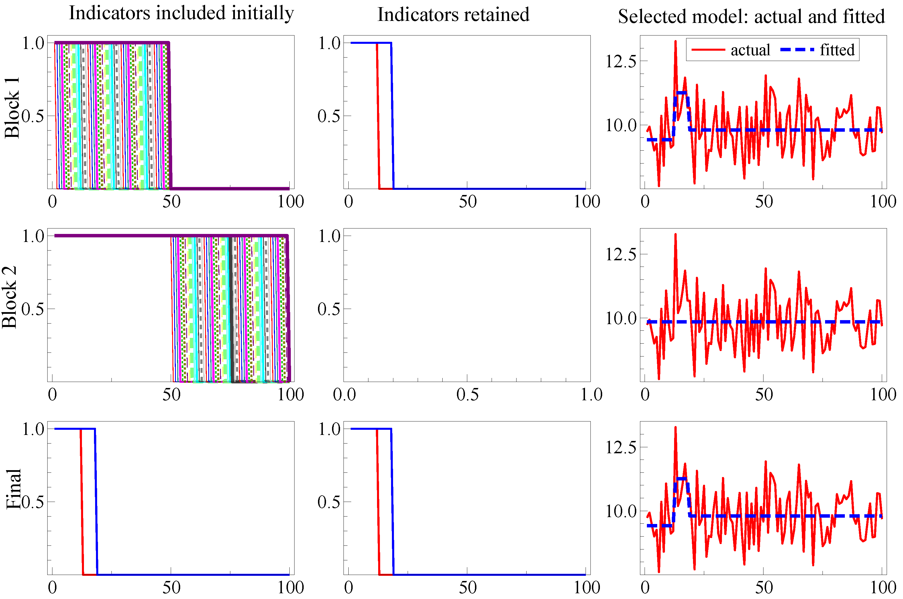
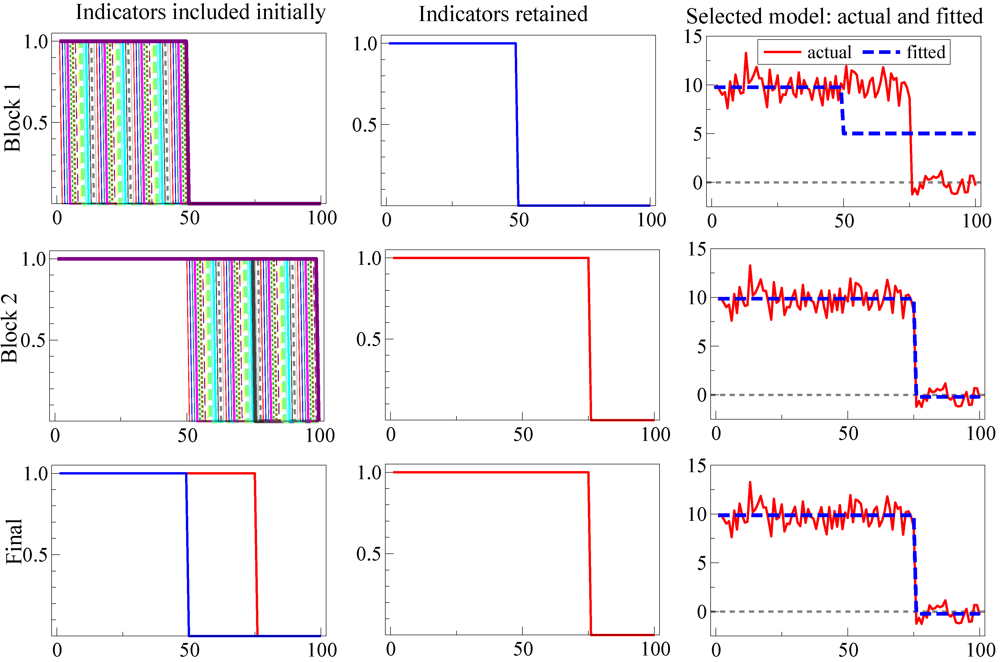
Figure 2 illustrates SIS for a location shift over the last 25 observations in the DGP:

$$y_t=\mu +{\lambda }_1{1}_{\left\{t\ge 76\right\}}+{ϵ}_t=10-10\times 1_{\left\{t\ge 76\right\}}+{ϵ}_t$$

(34)

where ${ϵ}_t\sim \mathsf{IN}\left[0,1\right]$. Initially, the last step indicator captures the mean shift drop (Row 1) matching the above analysis, then the location shift is found in Row 2, so the now redundant indicator is eliminated in Row 3. Thus, the outcome here coincides with the optimal test for a known location shift, namely a t-test in Equation (34) at $t=76$ onwards, without requiring knowledge: (1) that it was a location shift; (2) of the shift timing; (3) that it was the only shift; and (4) that the same magnitude of shift continued thereafter.

Figure 2. Illustrating split-half one-cut SIS for the shift in Equation (34).

Figure 2. Illustrating split-half one-cut SIS for the shift in Equation (34).

5.2. Simulating an Unknown Shift Period Matched by a Single Indicator

We now simulate the properties of SIS for a single location shift during the first half of the sample, using the DGP in Equation (11), where the timing of the location shift is set to $T_1=35$: varying shift lengths are investigated in Table 2. The shift magnitude ${\lambda }_1$ is set equal to $2{\sigma }_{ϵ}$ and $4{\sigma }_{ϵ}$, with selection at $\alpha =0.01$.

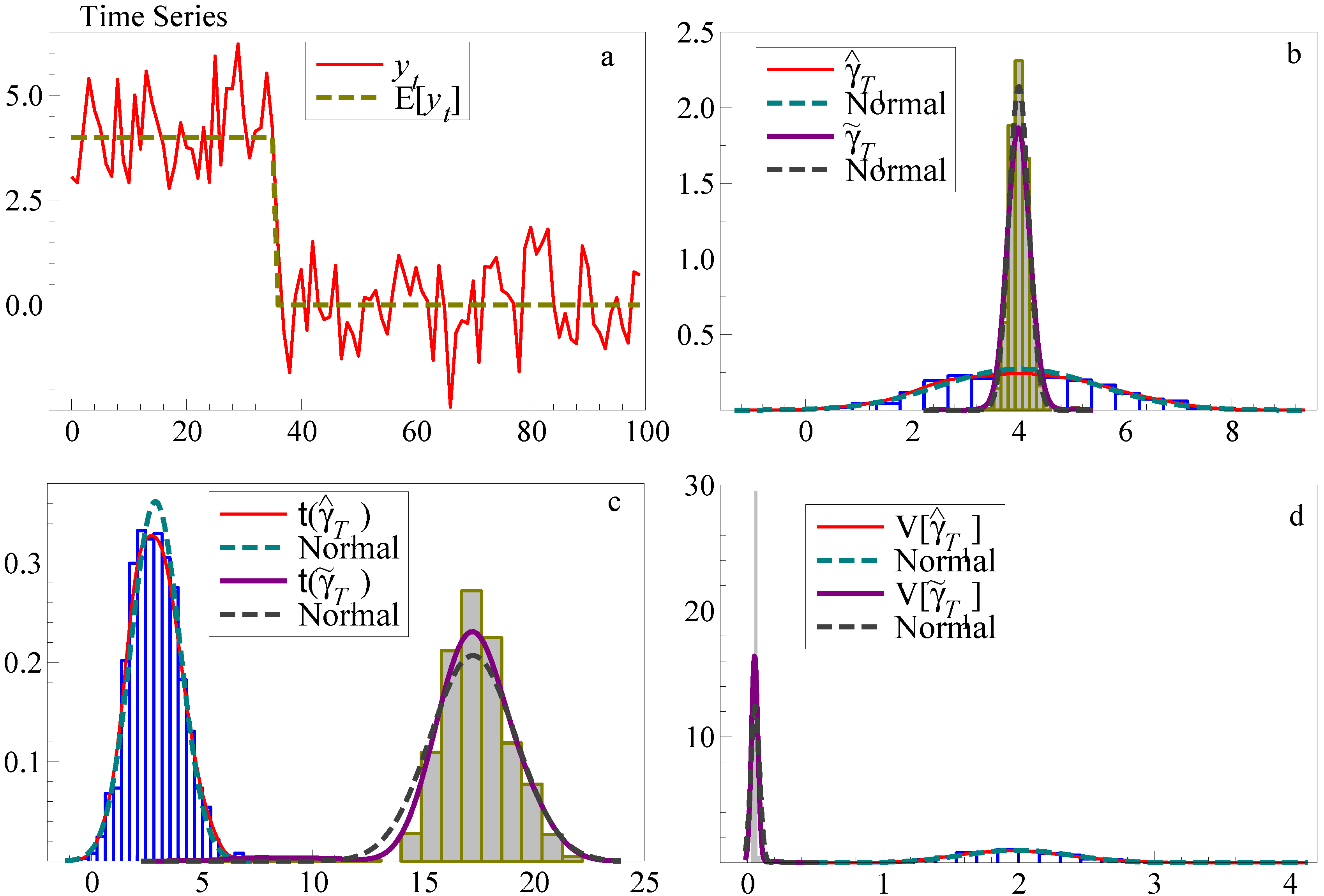
For the split-half one-cut approach outlined in Subsection 5.1, the open histograms and their densities in Figure 3b show that, while the density of ${\widehat{\gamma }}_{T_1}$ is centred around the true value of ${\lambda }_1$, in the case of $\mathsf{IID}$ errors, the variance of the estimator is twice that of the error (d), in line with Equation (23) below. The associated t-statistic density overlaps zero (c).

The retention frequencies of the step indicator $1_{\{t\le T_1\}}$ for varying lengths of shift and two levels of ${\lambda }_1$ without and with sequential selection of indicators are provided in Table 2. Given the relatively low retention frequency in the simple split-half one-cut approach, sequential selection of step indicators is essential. Iterative elimination of the least significant indicators leads to a rapid fall in the variance of the estimator $\mathsf{V}\left[{\tilde{\gamma }}_{T_1}\right]$ (Figure 3b, d), an increase in the retention frequency of the correct step indicators in (c) and a reduction in the number of incorrectly retained indicators. As the shaded histograms and their densities in Figure 3 and the lower section of Table 2 both show sequential selection or multi-path search as in Autometrics, this dramatically improves the outcomes of SIS in the single-shift experiment. For a step shift of $4{\sigma }_{ϵ}$, sequential selection increases the retention frequency on average to 0.93 from 0.59 with split-half one-cut.

Table 2. Retention frequency of ${\iota }_{T_1}$ for varying shift lengths l and magnitudes, ${\lambda }_1$, at $\alpha =0.01$.

Algorithm	${\lambda }_1$	$l=1$	$l=5$	$l=10$	$l=20$	$l=35$
Known shift:	$2{\sigma }_{ϵ}$	0.56 (2.77)	0.98 (4.72)	0.99 (6.27)	1.00 (8.17)	1.00 (9.65)
	$4{\sigma }_{ϵ}$	0.99 (5.59)	1.00 (9.50)	1.00 (12.57)	1.00 (16.36)	1.00 (19.31)
Split-half one-cut	$2{\sigma }_{ϵ}$	0.15 (1.43)	0.12 (1.42)	0.13 (1.47)	0.14 (1.44)	0.16 (1.47)
	$4{\sigma }_{ϵ}$	0.61 (2.88)	0.61 (2.88)	0.63 (2.92)	0.59 (2.88)	0.60 (2.92)
Split-half sequential:	$2{\sigma }_{ϵ}$	0.17 (3.01)	0.50 (3.68)	0.57 (4.63)	0.56 (5.86)	0.56 (6.92)
	$4{\sigma }_{ϵ}$	0.89 (4.10)	0.93 (6.81)	0.93 (8.96)	0.92 (11.62)	0.93 (13.70)
Multi-path	$2{\sigma }_{ϵ}$	0.41 (3.89)	0.57 (5.24)	0.57 (6.33)	0.58 (7.78)	0.55 (8.65)
	$4{\sigma }_{ϵ}$	0.95 (5.89)	0.93 (9.45)	0.95 (11.73)	0.93 (14.79)	0.92 (16.57)

Average t-values for retained indicators shown in parentheses.

Table 2. Retention frequency of ${\iota }_{T_1}$ for varying shift lengths l and magnitudes, ${\lambda }_1$, at $\alpha =0.01$.

Algorithm	${\lambda }_1$	$l=1$	$l=5$	$l=10$	$l=20$	$l=35$
Known shift:	$2{\sigma }_{ϵ}$	0.56 (2.77)	0.98 (4.72)	0.99 (6.27)	1.00 (8.17)	1.00 (9.65)
	$4{\sigma }_{ϵ}$	0.99 (5.59)	1.00 (9.50)	1.00 (12.57)	1.00 (16.36)	1.00 (19.31)
Split-half one-cut	$2{\sigma }_{ϵ}$	0.15 (1.43)	0.12 (1.42)	0.13 (1.47)	0.14 (1.44)	0.16 (1.47)
	$4{\sigma }_{ϵ}$	0.61 (2.88)	0.61 (2.88)	0.63 (2.92)	0.59 (2.88)	0.60 (2.92)
Split-half sequential:	$2{\sigma }_{ϵ}$	0.17 (3.01)	0.50 (3.68)	0.57 (4.63)	0.56 (5.86)	0.56 (6.92)
	$4{\sigma }_{ϵ}$	0.89 (4.10)	0.93 (6.81)	0.93 (8.96)	0.92 (11.62)	0.93 (13.70)
Multi-path	$2{\sigma }_{ϵ}$	0.41 (3.89)	0.57 (5.24)	0.57 (6.33)	0.58 (7.78)	0.55 (8.65)
	$4{\sigma }_{ϵ}$	0.95 (5.89)	0.93 (9.45)	0.95 (11.73)	0.93 (14.79)	0.92 (16.57)

Average t-values for retained indicators shown in parentheses.

Figure 3. Comparing SIS on a single shift without (open) and with (shaded) sequential selection. (a) shows the time series $y_t$ with a location shift; (b) and (c) the simulated estimator and test-statistic densities for split-half and sequential selection; and (d) their simulated variances.

Figure 3. Comparing SIS on a single shift without (open) and with (shaded) sequential selection. (a) shows the time series $y_t$ with a location shift; (b) and (c) the simulated estimator and test-statistic densities for split-half and sequential selection; and (d) their simulated variances.

Varying the shift length at the start of the sample appears to have little impact on the retention frequencies of the shift indicator, except in the case of a single impulse. Using split-half sequential selection, a shift of $2{\sigma }_{ϵ}$ is retained on average around 50% of the time, with an increase to around 90% for a shift of $4{\sigma }_{ϵ}$ (at $T=100$, $c_{0.01}=2.625$).

These simulations are consistent with the analysis in Subsection 5.1: the t-statistics for split-half one cut ${\widehat{\gamma }}_{T_1}$ in SIS are close to half those from IIS at the equivalent ${\lambda }_1$, but, with sequential simplification or multi-path search, converge to those for a known indicator. There is only a slight drop in retention frequency of the correct step at $4{\sigma }_{ϵ}$ despite searching over T indicators, though a rather larger drop at $2{\sigma }_{ϵ}$. Although the t-values of retained indicators increase with the shift length l, the retention probability remains relatively constant in all cases for $l>1$, possibly because we only record the retention of ${\iota }_{T_1}$, although a neighbouring indicator may have been found instead. Since the predictive failure test of [26] is based on IIS, as shown by [34], SIS should dominate the Chow test, yet not require knowledge of the shift point. IIS can already dominate [18], as shown in [10], so SIS multi-path should be a useful method for detecting and modelling location shifts.

5.3. Misspecified Indicator Timing

A step indicator selected in the marginal process may not exactly match the period characterizing a location shift because: (1) it ends after (or starts before); (2) it is a subset (so it starts after and ends before); and (3) it starts after and ends after (or starts before and ends before). Setting (1) is representative of the likely costs of misspecification, so we consider it in the special case just involving a shift and no other parameters. Let $1_{\left\{t\le T_0\right\}}$ denote the indicator where $T_0>T_1$, so that the marginal DGP is:

$$y_t={\gamma }_2+\lambda 1_{\left\{t\le T_1\right\}}+v_t\text{where}{v}_t\sim {\mathsf{N}}_{n_2}\left[0,{\omega }_v^2\right]$$

but now approximated by the incorrect model:

$$y_t=\mu +\theta 1_{\left\{t\le T_0\right\}}+u_t$$

with $\tau =T_1/T_0<1$. Autometrics selects congruent representations, so its step-indicator saturation algorithm will be directed away from non-overlapping indicators, like $1_{\left\{t\le T_0\right\}}$, when shifts are large or $T_0-T_1$ is long. Moreover, the costs of not matching dates precisely decline rapidly for small shifts. Similar analyses apply to Cases (2) and (3), with additional costs when parts of a shift are also not captured.

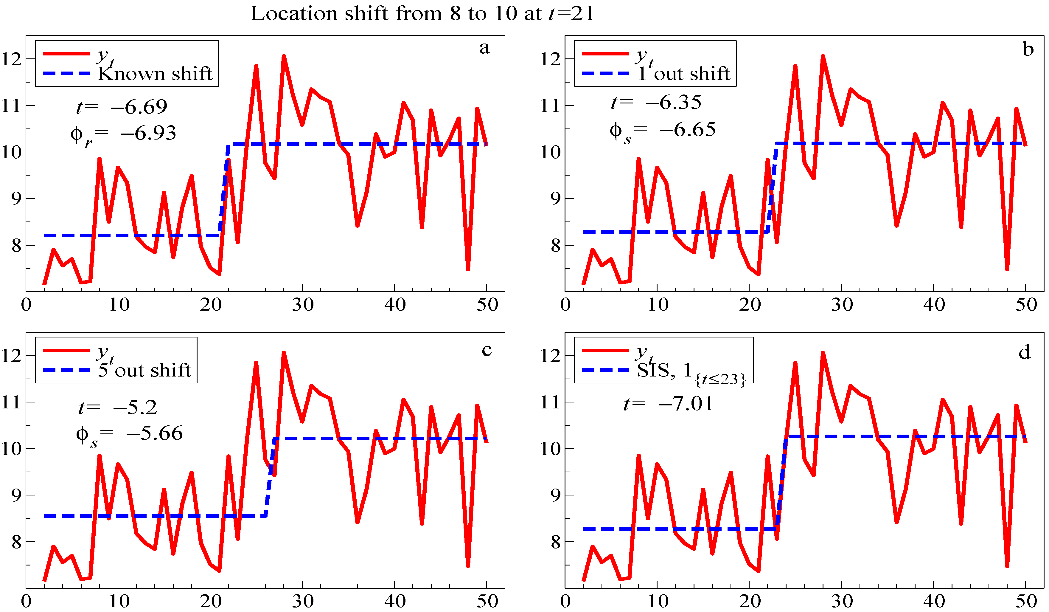
The choice of the period selected by SIS for a step indicator is because it has the largest t-statistic, so serious mismatches that leave large residuals are unlikely. To illustrate this, consider $y_t=10-2\times 1_{\left\{t\le 21\right\}}+{ϵ}_t$ where ${\sigma }_{ϵ}=1.0$, estimated for a known indicator as:

$$\begin{array}{ccc}\hfill {\widehat{y}}_t& =& \begin{array}{c}\hfill 10.2\\ \hfill {}^{(0.19)}\end{array}\begin{array}{c}-\\ \end{array}\begin{array}{c}\hfill 1.97\\ \hfill {}^{(0.29)}\end{array}\begin{array}{c}{1}_{\left\{t\le 21\right\}}\\ \end{array}\hfill \\ \hfill {\widehat{\sigma }}_{ϵ}& =& 1.012{\mathsf{F}}_{\mathsf{ar}}(2,45)=0.16{\mathsf{F}}_{\mathsf{het}}(1,47)=1.39{\chi }_{\mathsf{nd}}^2\left(2\right)=1.29\hfill \end{array}$$

The four panels in Figure 4 show the match to the data in one replication when the indicator is: (a) correct; (b) too long by one, (so $T_0=T_1+1$); (c) too long by five; and (d) selected by SIS, which picked $1_{\left\{t\le 23\right\}}$, but had the most significant outcome. The t-values are close to the theoretical non-centralities, ϕ as recorded in the figure. Moreover, although the SIS selection ‘misses’ by two periods, that is precisely because that is when the shift is shown most clearly, and the residuals for $t=21,22$ are not unusually large.

Figure 4. Fitted and actual values for four step-indicator specifications to a location shift at $t=21$. (a): known shift with t value and non-centrality ${\varphi }_r$; (b): shift approximated by a step one period late and (c): shift approximated by a step 5 periods late, both with non-centralities ${\varphi }_s$; and (d): SIS selection.

Figure 4. Fitted and actual values for four step-indicator specifications to a location shift at $t=21$. (a): known shift with t value and non-centrality ${\varphi }_r$; (b): shift approximated by a step one period late and (c): shift approximated by a step 5 periods late, both with non-centralities ${\varphi }_s$; and (d): SIS selection.

That the slow increase in potency shown in Table 2 is primarily due to slight mistiming rather than not detecting the shift is shown in Table 3. Potency increases monotonically down all columns, and even for $\lambda =2{\sigma }_{ϵ}$ and relatively short breaks, is 0.9 or higher by $T_1\pm 3$. However, unlike the ${\mathsf{F}}_{T-1}^1$-test non-centrality of $Tr\left(1-r\right){\lambda }^2/{\sigma }^2$ from analytic power calculations for a known break point exactly matched by the correct step function in a static regression, where r is the break-length fraction, potency does not increase much with $Tr\left(1-r\right)$. The results for $\lambda =4{\sigma }_{ϵ}$ are similar, but are not reported, as potency is near unity for all break lengths using $T_1\pm 1$.

Overall, SIS has relatively high potency for detecting a single location shift, albeit within a few periods on either side of its ending.

Table 3. Potency of $1_{\left\{t\le T_1\right\}}$ for varying break lengths $T_1$ and accuracy of timing using Autometrics.

$\lambda =2{\sigma }_{ϵ}$	$T_1=4$	$T_1=5$	$T_1=10$	$T_1=15$	$T_1=20$
$T_1$	0.58	0.55	0.59	0.59	0.59
$T_1\pm 1$	0.76	0.77	0.79	0.83	0.81
$T_1\pm 2$	0.84	0.87	0.86	0.90	0.89
$T_1\pm 3$	0.89	0.91	0.92	0.93	0.92

Table 3. Potency of $1_{\left\{t\le T_1\right\}}$ for varying break lengths $T_1$ and accuracy of timing using Autometrics.

$\lambda =2{\sigma }_{ϵ}$	$T_1=4$	$T_1=5$	$T_1=10$	$T_1=15$	$T_1=20$
$T_1$	0.58	0.55	0.59	0.59	0.59
$T_1\pm 1$	0.76	0.77	0.79	0.83	0.81
$T_1\pm 2$	0.84	0.87	0.86	0.90	0.89
$T_1\pm 3$	0.89	0.91	0.92	0.93	0.92

5.4. Unknown Shift Requiring a Two-Step Indicator in One-Half Sample

An unknown location shift may require a two-step indicator, as in the following DGP:

$$y_t=\lambda \left(1_{\left\{t\le T_2\right\}}-1_{\left\{t\le T_1\right\}}\right)+{ϵ}_t\text{where}{ϵ}_t\sim \mathsf{IN}\left[0,{\sigma }_{ϵ}^2\right]$$

(35)

where $\lambda \ne 0$, and $T_1<T_2<T/2$, so as in Subsection 5.1, the shift is entirely within one-half of the sample. The model for the first-half split is:

$$\mathbf{y}={\mathbf{D}}_1{\gamma }_{\left(1\right)}+\mathbf{v}$$

(36)

where ${\gamma }_{\left(1\right)}={({\gamma }_1\dots {\gamma }_{T/2})}^{\prime }$ and ${\mathbf{D}}_1=({\iota }_1\dots {\iota }_{T/2})$. For Equation (36) estimated on data from Equation (35):

$$\begin{array}{cc}\hfill {\tilde{\gamma }}_{\left(1\right)}& ={\left({\mathbf{D}}_1^{\prime }{\mathbf{D}}_1\right)}^{-1}{\mathbf{D}}_1^{\prime }\mathbf{y}\hfill \\ & =\lambda {\left({\mathbf{D}}_1^{\prime }{\mathbf{D}}_1\right)}^{-1}{\mathbf{D}}_1^{\prime }\left({\iota }_{T_2}-{\iota }_{T_1}\right)+{\left({\mathbf{D}}_1^{\prime }{\mathbf{D}}_1\right)}^{-1}{\mathbf{D}}_1^{\prime }ϵ\hfill \\ & =\lambda \mathbf{s}+\nabla {ϵ}_{\left(1\right)}\hfill \end{array}$$

(37)

where s is a $T/2\times 1$ selection vector with unity in the $T_2$-th position, $-1$ in the $T_1$-th position and zeroes elsewhere. Thus, a similar analysis to Subsection 5.1 holds for two relevant indicators, with r replaced by s, so selecting indicators in the latter half of the sample should remain as before.

To simulate an unknown shift period requiring a two-step indicator in the first-half, we set $T_1=25$ and $T_2=35$, and only consider sequentially selected indicators here, retaining the selected indicators from ${\mathbf{D}}_1$ and ${\mathbf{D}}_2$ at $\alpha =0.01$. Table 4 shows the simulation results for sequential selection from the split-half for two shifts, so retention frequencies are close to the case of a single shift.

Table 4. Split-half sequential selection: gauge and retention frequencies for a shift with two indicators.

	Gauge		Retention frequency
${\lambda }_1$	${\mathbf{D}}_1$	${\mathbf{D}}_2$	$T_1$ step	$T_2$ step
$2{\sigma }_{ϵ}$	0.020	0.011	0.52	0.55
$4{\sigma }_{ϵ}$	0.004	0.017	0.91	0.94

Table 4. Split-half sequential selection: gauge and retention frequencies for a shift with two indicators.

	Gauge		Retention frequency
${\lambda }_1$	${\mathbf{D}}_1$	${\mathbf{D}}_2$	$T_1$ step	$T_2$ step
$2{\sigma }_{ϵ}$	0.020	0.011	0.52	0.55
$4{\sigma }_{ϵ}$	0.004	0.017	0.91	0.94

5.5. Unknown Opposite-Signed Shifts in Each Split Half

If shifts in each half of the sample have opposite signs, or perhaps very different magnitudes, then both can be detected even in a split-half sequential selection approach. Consider the DGP:

$$y_t={\lambda }_1\left(1_{\left\{t\le T_2\right\}}-1_{\left\{t\le T_1\right\}}\right)+{\lambda }_2\left(1_{\left\{t\le T_4\right\}}-1_{\left\{t\le T_3\right\}}\right)+{ϵ}_t$$

(38)

where ${ϵ}_t\sim \mathsf{IN}\left[0,{\sigma }_{ϵ}^2\right]$ as before, and $T_1<T_2\le T/2$, whereas $T/2\le T_3<T_4$ with ${\lambda }_1{\lambda }_2<0$. To remove the mean effect of the other location shift, since:

$$\frac{1}{T}\sum _{t=1}^T\left({\lambda }_2\left(1_{\left\{t\le T_4\right\}}-1_{\left\{t\le T_3\right\}}\right)\right)={\lambda }_2\frac{\left(T_4-T_3\right)}{T}={\varphi }_2,$$

the intercept must be retained without selection.

The formula in (37) still applies, with appropriate adjustments for estimating the intercepts, but even if the first shift is correctly modelled, the equation in (22) for the residuals becomes:

$$\mathbf{y}-\widehat{\mathbf{y}}={\lambda }_2\left({\iota }_{T_4}-{\iota }_{T_3}\right)-{\varphi }_2\iota +{ϵ}_2^{*}={\widehat{\mathbf{v}}}_2$$

(39)

which has a larger estimated error variance than in the previous cases, because:

$$\begin{array}{cc}\hfill \frac{2}{T}\mathsf{E}\left[{\widehat{\mathbf{v}}}_2^{\prime }{\widehat{\mathbf{v}}}_2\right]& =\frac{2}{T}\mathsf{E}\left[{\left({ϵ}_2^{*}\right)}^{\prime }{ϵ}_2^{*}\right]+\frac{2}{T}{\left({\lambda }_2\left({\iota }_{T_4}-{\iota }_{T_3}\right)-{\varphi }_2\iota \right)}^{\prime }\left({\lambda }_2\left({\iota }_{T_4}-{\iota }_{T_3}\right)-{\varphi }_2\iota \right)\hfill \\ & ={\sigma }_{ϵ}^2+{\lambda }_2^2\frac{2\left(T_4-T_3\right)}{T}-2{\lambda }_2{\varphi }_2\frac{2\left(T_4-T_3\right)}{T}+2{\varphi }_2^2\hfill \\ & ={\sigma }_{ϵ}^2+2{\lambda }_2^2\frac{\left(T_4-T_3\right)}{T}\left(1-\frac{\left(T_4-T_3\right)}{T}\right)\hfill \end{array}$$

(40)

To compensate for the equivalent effect of Equation (40), when searching for a second shift, step indicators found in the first half should be be included in the second-half selection.

To simulate unknown opposite-signed shifts in each half, ${\lambda }_1$ and ${\lambda }_2$ are chosen, such that ${\lambda }_1=-{\lambda }_2$, where the shift timing is given by $T_1=25$ to $T_2=35$ and $T_3=75$ to $T_4=85$. Table 5 shows that even with shifts falling in the middle of each half, SIS can be successful in identifying the shift points.

Table 5. Split-half sequential selection: opposite-signed shifts in each half, $\alpha =0.01$.

	Gauge		Retention frequency
${\lambda }_{1,2}$	${\mathbf{D}}_1$	${\mathbf{D}}_2$	$T_1$ step	$T_2$ step	$T_3$ step	$T_4$ step
$2{\sigma }_{ϵ}$	0.021	0.045	0.52	0.55	0.57	0.56
$4{\sigma }_{ϵ}$	0.004	0.030	0.91	0.94	0.93	0.93

Table 5. Split-half sequential selection: opposite-signed shifts in each half, $\alpha =0.01$.

	Gauge		Retention frequency
${\lambda }_{1,2}$	${\mathbf{D}}_1$	${\mathbf{D}}_2$	$T_1$ step	$T_2$ step	$T_3$ step	$T_4$ step
$2{\sigma }_{ϵ}$	0.021	0.045	0.52	0.55	0.57	0.56
$4{\sigma }_{ϵ}$	0.004	0.030	0.91	0.94	0.93	0.93

5.6. Unknown Equal Shifts in Each Split Half

Shifts with relatively equal magnitudes, durations and the same signs in each half, so they are roughly evenly distributed between the two halves, could well appear as just a larger error variance, rendering the simplest split-half one-cut approach ineffective. Nevertheless, when T is sufficiently large, both shifts can be detected using a modified split-half approach. First, saturate the second half by impulse indicators, then the first half can be tackled by a split-half approach, so quarters are examined, without any additional cost under the null. That procedure is then reversed for the first half. This is a variant of super saturation, where IIS is also undertaken with SIS as in [15], but here limiting IIS to the alternate half and not using the information it reveals about outliers and shifts.

Under the alternative, by eliminating the shift in the second half, the first half comes under the above analysis for a single shift, which is then detectable provided it is not evenly split between the quarters. In practice, Autometrics uses multiple block searches, and this has proven effective for IIS in detecting multiple shifts. Blocks would need to span most of the length of a location shift to detect it using SIS, but that may be less essential for super saturation.

Unknown shifts of equal magnitude are assessed by setting ${\lambda }_1={\lambda }_2$, with $T_1=25$ to $T_2=35$ and $T_3=75$ to $T_4=85$, so there are two same-sign step shifts of equal magnitude and length in each half. We consider both the split-half sequential selection approach and multi-path selection using Autometrics (where a single gauge value is reported for ${\mathbf{D}}_1$ and ${\mathbf{D}}_2$). Table 6 provides summary results showing little difference in retention frequencies.

Table 6. Split-half sequential selection and multi-path: unknown equal shifts in each half, $\alpha =0.01$.

Algorithm	Gauge		Retention Frequency
${\lambda }_1$	${\mathbf{D}}_1$	${\mathbf{D}}_2$	$T_1$ step	$T_2$ step	$T_3$ step	$T_4$ step
Sequential: $2{\sigma }_{ϵ}$	0.021	0.044	0.52	0.55	0.59	0.60
$4{\sigma }_{ϵ}$	0.005	0.030	0.91	0.94	0.94	0.94
${\lambda }_1$	${\mathbf{D}}_1$ & ${\mathbf{D}}_2$		$T_1$ step	$T_2$ step	$T_3$ step	$T_4$ step
Multi-path: $2{\sigma }_{ϵ}$	0.038		0.53	0.48	0.55	0.55
$4{\sigma }_{ϵ}$	0.018		0.87	0.91	0.94	0.92

Table 6. Split-half sequential selection and multi-path: unknown equal shifts in each half, $\alpha =0.01$.

Algorithm	Gauge		Retention Frequency
${\lambda }_1$	${\mathbf{D}}_1$	${\mathbf{D}}_2$	$T_1$ step	$T_2$ step	$T_3$ step	$T_4$ step
Sequential: $2{\sigma }_{ϵ}$	0.021	0.044	0.52	0.55	0.59	0.60
$4{\sigma }_{ϵ}$	0.005	0.030	0.91	0.94	0.94	0.94
${\lambda }_1$	${\mathbf{D}}_1$ & ${\mathbf{D}}_2$		$T_1$ step	$T_2$ step	$T_3$ step	$T_4$ step
Multi-path: $2{\sigma }_{ϵ}$	0.038		0.53	0.48	0.55	0.55
$4{\sigma }_{ϵ}$	0.018		0.87	0.91	0.94	0.92

5.7. Unknown Shift Period Spanning Both Splits

The analysis in Subsection 5.6 may be effective in capturing a location shift spanning the initial halves, as then the shift will almost always lie entirely within a quarter of the sample. This follows, since within the first half of $T/2$ where the shift lies towards the end by necessity of spanning into the second half, if it were longer than $T/4$, SIS would find the shorter as if it were the shift and similarly for the second half.

To simulate a shift period spanning both splits, the shift timing is set such that the end of the first shift occurs just as the second shift starts, i.e., $T_2=T/2$ and $T_3=T/2+1$ with $T_1=35$ and $T_4=65$, leading to a single step shift of a length of 30 periods spanning both halves. Table 7 presents the results when using split-half sequential selection, as well as multi-path. Both correctly show the absence of shifts at $T_2$ and $T_3$ (as the shift spans the two halves), and as before, there is little difference between these, exhibiting retention frequencies at $T_1$ and $T_4$ of around 0.9 for a step shift of $4{\sigma }_{ϵ}$.

Table 7. Split-half sequential sequential and multi-path: shift spanning both splits, $\alpha =0.01$.

Algorithm	Gauge		Retention frequency
${\lambda }_1$	${\mathbf{D}}_1$	${\mathbf{D}}_2$	$T_1$ Step	$T_2$ Step	$T_3$ Step	$T_4$ Step
Sequential: $2{\sigma }_{ϵ}$	0.011	0.039	0.58	0.001	0.0	0.56
$4{\sigma }_{ϵ}$	0.002	0.02	0.94	0.0	0.0	0.93
${\lambda }_1$	${\mathbf{D}}_1$ & ${\mathbf{D}}_2$		$T_1$ Step	$T_2$ Step	$T_3$ Step	$T_4$ Step
Multi-path: $2{\sigma }_{ϵ}$	0.029		0.57	0.01	0.01	0.55
$4{\sigma }_{ϵ}$	0.019		0.94	0.02	0.02	0.96

Table 7. Split-half sequential sequential and multi-path: shift spanning both splits, $\alpha =0.01$.

Algorithm	Gauge		Retention frequency
${\lambda }_1$	${\mathbf{D}}_1$	${\mathbf{D}}_2$	$T_1$ Step	$T_2$ Step	$T_3$ Step	$T_4$ Step
Sequential: $2{\sigma }_{ϵ}$	0.011	0.039	0.58	0.001	0.0	0.56
$4{\sigma }_{ϵ}$	0.002	0.02	0.94	0.0	0.0	0.93
${\lambda }_1$	${\mathbf{D}}_1$ & ${\mathbf{D}}_2$		$T_1$ Step	$T_2$ Step	$T_3$ Step	$T_4$ Step
Multi-path: $2{\sigma }_{ϵ}$	0.029		0.57	0.01	0.01	0.55
$4{\sigma }_{ϵ}$	0.019		0.94	0.02	0.02	0.96

5.8. Summary of the Simulation Results

The Monte Carlo experiments provide evidence for the feasibility of detecting location shifts using SIS. In the case of static DGPs with specific location shifts, the step indicators exhibit high retention frequencies: around 50% in the case of a shift equal to two standard deviations and around 90% for shifts of four standard deviations. These results hold across single shifts, multiple shifts of the same or opposite signs and shifts spanning both halves. Sequential selection of step shifts is crucial to ensure high potency when using split half, which, in turn, requires any selected indicators to be carried forward into the second set of indicators. Multi-path search using Autometrics without the condition of carrying relevant indicators forward yields similar results to split-half sequential simplification. Overall, the results match the theoretical analyses of gauge and potency for a single shift, noting that gauge is higher for SIS than IIS as 2 steps are needed to characterize a single outlier.

6. Generalization to Retained Regressors

Following the theoretical findings in [4] for IIS, we use simulations to assess SIS with $n<T/2$ general regressors by including the $T\times n$ matrix Z as independent variables. For a single-step shift with unknown timing requiring two indicators, the DGP is then given by:

$$y_t={\beta }_1^{\prime }{\mathbf{z}}_t+\lambda \left(1_{\left\{t\le T_2\right\}}-1_{\left\{t\le T_1\right\}}\right)+{ϵ}_t\text{where}{ϵ}_t\sim \mathsf{IN}\left[0,{\sigma }_{ϵ}^2\right]$$

(41)

For the present simulation, we set ${\sigma }_{ϵ}^2=1$ and $n=10$. For each of the $i=1,\dots ,n\mathsf{IID}$ IID regressors, the associated non-centralities are set to $\mathsf{E}\left[{\mathsf{t}}_i\right]={\psi }_i=4$. The individual $z_i$ are orthogonal in expectation and not selected over (see [27]), so they are present in every selection iteration of the step indicators. The shift timing is set as before to $T_1=25$ and $T_2=35$.

Table 8 displays the simulation outcomes and properties of the step indicators. With the inclusion of 10 relevant independent variables, the densities of the two shift estimators are centred around the true value of ${\lambda }_1=4{\sigma }_{ϵ}$. The potency of SIS seems unaffected by the presence of additional fixed regressors, with retention frequencies close to those in experiments without regressors.

Table 8. SIS with regressors.

	Gauge	Retention frequency
${\lambda }_1$		$T_1$ step	$T_2$ step
$2{\sigma }_{ϵ}$	0.035	0.50	0.62
$4{\sigma }_{ϵ}$	0.024	0.91	0.94

Table 8. SIS with regressors.

	Gauge	Retention frequency
${\lambda }_1$		$T_1$ step	$T_2$ step
$2{\sigma }_{ϵ}$	0.035	0.50	0.62
$4{\sigma }_{ϵ}$	0.024	0.91	0.94

7. Comparisons with Least Angle Regression

Simulation results for LARS (see [23]) use the same DGPs as for SIS in Subsection 3, based on $M=$ 1000 replications at $T=100$. Findings under the null of no shifts are reported in Table 9, where Table 1 recorded the gauge of SIS.

Table 9. Null retention frequency of least angle regression (LARS) under the null of no shifts.

LARS Step	1	2	3	4	5	Cross-Validated
Gauge	0.029	0.047	0.061	0.073	0.084	0.017

Table 9. Null retention frequency of least angle regression (LARS) under the null of no shifts.

LARS Step	1	2	3	4	5	Cross-Validated
Gauge	0.029	0.047	0.061	0.073	0.084	0.017

Under the null, the gauge is difficult to control for different steps in the LARS algorithm and quickly exceeds the gauge of SIS, as seen in Table 9. However, cross-validation under the null yields a gauge close to SIS at 1%.

Under the alternative, the gauge can vary drastically. Table 10 applies the cross-validated LARS step for single shifts with varying lengths, whereas Table 11 and Table 12 consider multiple shifts. For a single shift, the potency for exact detection in Table 10 is high, as expected for a single-step forward search procedure. Like SIS, there is little apparent potency increase with the length of shift, but that probably reflects mistiming rather than missing the shift, as occurred for SIS in Table 3. The gauge for a single shift between 2% and 6% is higher than under the null.

Overall, while LARS exhibits high potency, this is the result of a high gauge that is difficult to control, varying from 1.7% under the null, to 16.7% facing multiple shifts. This makes it difficult to use LARS in practice, as the number of shifts is not generally known a-priori.

Table 10. Potency and gauge of cross-validated LARS for single shifts of lengths l and magnitudes ${\lambda }_1$.

	${\lambda }_1$	$l=1$	$l=5$	$l=10$	$l=20$	$l=35$
Potency	$2{\sigma }_{ϵ}$	0.298	0.800	0.844	0.853	0.854
Potency	$4{\sigma }_{ϵ}$	0.780	0.990	0.990	0.996	1.00
Gauge	$2{\sigma }_{ϵ}$	0.018	0.050	0.054	0.056	0.058
Gauge	$4{\sigma }_{ϵ}$	0.020	0.052	0.055	0.058	0.059

Table 10. Potency and gauge of cross-validated LARS for single shifts of lengths l and magnitudes ${\lambda }_1$.

	${\lambda }_1$	$l=1$	$l=5$	$l=10$	$l=20$	$l=35$
Potency	$2{\sigma }_{ϵ}$	0.298	0.800	0.844	0.853	0.854
Potency	$4{\sigma }_{ϵ}$	0.780	0.990	0.990	0.996	1.00
Gauge	$2{\sigma }_{ϵ}$	0.018	0.050	0.054	0.056	0.058
Gauge	$4{\sigma }_{ϵ}$	0.020	0.052	0.055	0.058	0.059

Table 11. Potency and gauge of cross-validated LARS for same-sign, equal-magnitude shifts over $T_1=25$ to $T_2=35$ and $T_3=75$ to $T_4=85$.

${\lambda }_1$	gauge	$T_1$ potency	$T_2$ potency	$T_3$ potency	$T_4$ potency
$2{\sigma }_{ϵ}$	0.167	0.829	0.839	0.871	0.818
$4{\sigma }_{ϵ}$	0.166	0.997	1.00	1.00	0.992

Table 11. Potency and gauge of cross-validated LARS for same-sign, equal-magnitude shifts over $T_1=25$ to $T_2=35$ and $T_3=75$ to $T_4=85$.

${\lambda }_1$	gauge	$T_1$ potency	$T_2$ potency	$T_3$ potency	$T_4$ potency
$2{\sigma }_{ϵ}$	0.167	0.829	0.839	0.871	0.818
$4{\sigma }_{ϵ}$	0.166	0.997	1.00	1.00	0.992

Table 12. Potency and gauge of cross-validated LARS for equal magnitude, opposite-signed shifts over $T_1=25$ to $T_2=35$ and $T_3=75$ to $T_4=85$.

${\lambda }_1$	gauge	$T_1$ potency	$T_2$ potency	$T_3$ potency	$T_4$ potency
$2{\sigma }_{ϵ}$	0.164	0.836	0.837	0.857	0.867
$4{\sigma }_{ϵ}$	0.160	0.997	1.00	0.998	0.997

Table 12. Potency and gauge of cross-validated LARS for equal magnitude, opposite-signed shifts over $T_1=25$ to $T_2=35$ and $T_3=75$ to $T_4=85$.

${\lambda }_1$	gauge	$T_1$ potency	$T_2$ potency	$T_3$ potency	$T_4$ potency
$2{\sigma }_{ϵ}$	0.164	0.836	0.837	0.857	0.867
$4{\sigma }_{ϵ}$	0.160	0.997	1.00	0.998	0.997

8. Non-Linearity and SIS

When the DGP, or models thereof, include non-linear transformations of variables, the issue arises as to whether also applying SIS will affect the selection of the correct formulation. We consider three possibilities when selecting non-linearity:

(1)

the DGP includes non-linear variables, but no shifts, and SIS is applied;

(2)

there is a shift in the dependent variable, but no non-linearity and SIS is not applied; and

(3)

Setting (2), but SIS is applied.

First, consider a simple static DGP without shifts, but containing non-linear variables, as given in Equation (42):

$$y_t=\mu +{\beta }_1{x}_t+{\beta }_2{x}_t^2+{\beta }_3{x}_t^3+{ϵ}_t\text{where}{ϵ}_t\sim \mathsf{IN}[0,1]$$

(42)

and for convenience, $x_t\sim \mathsf{IN}[0,1]$, when the non-centralities associated with the three explanatory variables are ${\psi }_i=3$ for $i=1,2,3$. The model is also given by Equation (42), where all variables are first retained without SIS, then subject to selection jointly with SIS.

In Table 13, we report the effect on the null rejection frequencies of t-tests for the correctly included non-linear variables when not selected over, as well as the retention frequency when the relevant variables are selected over jointly with SIS. Simulations are reported for a sample of $T=100$ using $M=$ 1,000 replications, with variables being selected at $\alpha =0.01$. Inclusion of a saturating set of step indicators in the candidates has little effect on the null retention frequencies of indicators and non-null retention frequencies of relevant non-linear variables when there is no shift. When $x_t^k,k=1,2,3$ are always retained, the null rejection frequencies at 1% are close to the theory level of $\approx 0.66$, though somewhat higher when SIS is used due to slight under-estimation of the error variance. When the $x_t^k$ are jointly selected with SIS, the retention drops marginally relative to the no-SIS case.

Table 13. The effect of using SIS in Equation (42) on the rejection frequencies when the $x_t^k$ are always retained and retention frequencies when they are selected over (both at 1%).

Variable	Null rejection at 1% (xs retained)		Retention at 1% (x’s selected over)
	without SIS	with SIS	without SIS	with SIS
x, $\psi =3$	0.65	0.68	0.68	0.63
$x^2$, $\psi =3$	0.64	0.67	0.68	0.56
$x^3$, $\psi =3$	0.65	0.68	0.67	0.62
SIS gauge	-	0.02	-	0.03

Table 13. The effect of using SIS in Equation (42) on the rejection frequencies when the $x_t^k$ are always retained and retention frequencies when they are selected over (both at 1%).

Variable	Null rejection at 1% (xs retained)		Retention at 1% (x’s selected over)
	without SIS	with SIS	without SIS	with SIS
x, $\psi =3$	0.65	0.68	0.68	0.63
$x^2$, $\psi =3$	0.64	0.67	0.68	0.56
$x^3$, $\psi =3$	0.65	0.68	0.67	0.62
SIS gauge	-	0.02	-	0.03

Second, we study the effect of SIS when there is a shift in the dependent variable $y_t$, such that a non-linear transformation of the explanatory variables may spuriously appear significant by approximating this break. The example considered here is for the DGP given in Equation (43):

$$y_t=\mu +\lambda 1_{\{t\ge 35\}}+{ϵ}_t$$

(43)

The estimated model is identical to that given in Equation (42), except that now the $x_t$ variable is generated such that a non-linear transformation spuriously approximates the structural break in Equation (43). For illustration, $x_t$ is generated with the functional form $x_t={|\gamma {\left(1+\kappa e^{-rt}\right)}^{-1}+v_t|}^{(1/3)}$, where $\gamma =10$, $\kappa =70$, $r=0.1$ and $v_t\sim \mathsf{IN}[0,1]$. The results are recorded in Table 14, both when $x_t^k$ are always retained and when selected over jointly with SIS.

Table 14. The impact of SIS in Equation (42) on the null rejection frequencies of $x_t^k$, which are always retained, and the retention frequencies when they are selected over, with and without SIS in the presence of a step-shift ${\lambda }_1$ at $T_1=35$ (all at 1%).

Variable	Null rejection at 1% (xs retained)				Retention at 1% (xs selected over)
	${\lambda }_1=2{\sigma }_{ϵ}$		${\lambda }_1=4{\sigma }_{ϵ}$		${\lambda }_1=2{\sigma }_{ϵ}$		${\lambda }_1=4{\sigma }_{ϵ}$
	no SIS	with SIS	no SIS	with SIS	no SIS	with SIS	no SIS	with SIS
x, $\psi =0$	0.22	0.06	0.73	0.03	0.41	0.02	0.83	0.02
$x^2$, $\psi =0$	0.29	0.06	0.87	0.03	0.66	0.02	0.96	0.02
$x^3$, $\psi =0$	0.26	0.06	0.80	0.02	0.30	0.02	0.83	0.01
$T_1$ step	-	0.51	-	0.93	-	0.62	-	0.94
SIS gauge	-	0.02	-	0.02	-	0.02	-	0.02

Table 14. The impact of SIS in Equation (42) on the null rejection frequencies of $x_t^k$, which are always retained, and the retention frequencies when they are selected over, with and without SIS in the presence of a step-shift ${\lambda }_1$ at $T_1=35$ (all at 1%).

Variable	Null rejection at 1% (xs retained)				Retention at 1% (xs selected over)
	${\lambda }_1=2{\sigma }_{ϵ}$		${\lambda }_1=4{\sigma }_{ϵ}$		${\lambda }_1=2{\sigma }_{ϵ}$		${\lambda }_1=4{\sigma }_{ϵ}$
	no SIS	with SIS	no SIS	with SIS	no SIS	with SIS	no SIS	with SIS
x, $\psi =0$	0.22	0.06	0.73	0.03	0.41	0.02	0.83	0.02
$x^2$, $\psi =0$	0.29	0.06	0.87	0.03	0.66	0.02	0.96	0.02
$x^3$, $\psi =0$	0.26	0.06	0.80	0.02	0.30	0.02	0.83	0.01
$T_1$ step	-	0.51	-	0.93	-	0.62	-	0.94
SIS gauge	-	0.02	-	0.02	-	0.02	-	0.02

When there is a shift in the dependent variable that renders non-linear variables significant, SIS is able to pick up the shift that is otherwise attributed to non-linearity in the model. By detecting the shift, the null rejection (and retention) frequencies of the irrelevant non-linear variables is moved much closer to the nominal level, and for a $4{\sigma }_{ϵ}$ shift, using SIS reduces the null rejection frequency for the irrelevant $x_t^k$ from around 0.8 to 0.02–0.03 when testing at $1\%$. This result is robust to whether the $x_t^k$ are always retained or are selected over. The potency of detecting the shift using SIS is also not affected by the presence of non-linear covariates and is close to that found in previous sections, namely $\approx 0.5$ for a $2{\sigma }_{ϵ}$ shift and $\approx 0.9$ for $4{\sigma }_{ϵ}$.

Thus, SIS can act as an insurance mechanism in non-linear models. If there are non-linearities present in the DGP, employing SIS has little effect on the null rejection and retention frequencies, and the gauge is close to the nominal significance level. If there are unknown shifts in the dependent variable that may otherwise be attributed to non-linearities, SIS exhibits high potency in identifying the shift and restores the null rejection and retention frequencies of the irrelevant non-linear variables close to the nominal value.

9. Conclusion

Detecting location shifts by step-indicator saturation has the correct null retention frequency in constant conditional models for a nominal selection size of α. The approximate alternative retention frequency function was derived analytically for simple models and helps explain the simulation outcomes. Although only one and two shifts were considered in detail, the general nature of the approach makes it applicable when there are multiple shifts. There have already been a number of applications of SIS to empirical problems, including commodity price shifts in [35], location shifts in U.K. real wage determination in [21] and detecting crises in [15], as well as variants to measure the impacts of volcanic eruptions on temperature in [30]. Non-linearities that are relevant are not ‘lost’ by using SIS, whereas irrelevant, but spuriously significant ones can be eliminated by SIS.

While all of the derivations and Monte Carlo experiments here have been for simple static equations and specific location shifts, the principles seem general and should apply to dynamic equations (although with approximate null-retention frequencies) and to conditional systems. Generalizations to non-stationary settings would need to extend the analysis in [4]. Other important new analyses for SIS are checking for location shifts at the forecast origin, which would otherwise be pernicious for forecast accuracy, and to testing super exogeneity, where the IIS-based test in [5] has relatively low power for long shifts.

References

1. J.L. Castle, and D.F. Hendry. “Model selection in under-specified equations with breaks.” J. Econ. 178 (2014): 286–293. [Google Scholar] [CrossRef]
2. M.P. Clements, and D.F. Hendry. Forecasting Economic Time Series. Cambridge, UK: Cambridge University Press, 1998. [Google Scholar]
3. D.F. Hendry, S. Johansen, and C. Santos. “Automatic selection of indicators in a fully saturated regression.” Comput. Stat. 33 (2008): 317–335. Erratum, 337–339. [Google Scholar] [CrossRef]
4. S. Johansen, and B. Nielsen. “An analysis of the indicator saturation estimator as a robust regression estimator.” In The Methodology and Practice of Econometrics. Edited by J.L. Castle and N. Shephard. Oxford, UK: Oxford University Press, 2009, pp. 1–36. [Google Scholar]
5. D.F. Hendry, and C. Santos. “An automatic test of super exogeneity.” In Volatility and Time Series Econometrics. Edited by M.W. Watson, T. Bollerslev and J. Russell. Oxford, UK: Oxford University Press, 2010, pp. 164–193. [Google Scholar]
6. R.F. Engle, D.F. Hendry, and J.F. Richard. “Exogeneity.” Econometrica 51 (1983): 277–304. [Google Scholar] [CrossRef]
7. D.F. Hendry, and G.E. Mizon. “Econometric modelling of time series with outlying observations.” J. Time Series Econ. 3 (2011). [Google Scholar] [CrossRef]
8. J.J. Reade, and U. Volz. “From the general to the specific: Modelling inflation in China.” Appl. Econ. Q. 7 (2011): 27–44. [Google Scholar] [CrossRef]
9. N.R. Ericsson, and E.L. Reisman. “Evaluating a global vector autoregression for forecasting.” Int. Adv. Econ. Res. 18 (2012): 247–258. [Google Scholar] [CrossRef]
10. J.L. Castle, J.A. Doornik, and D.F. Hendry. “Model selection when there are multiple breaks.” J. Econ. 169 (2012): 239–246. [Google Scholar] [CrossRef]
11. D.F. Hendry, and F. Pretis. “Anthropogenic influences on atmospheric CO2.” In Handbook on Energy and Climate Change. Edited by R. Fouquet. Cheltenham, UK: Edward Elgar, 2013, pp. 287–326. [Google Scholar]
12. N.R. Ericsson. “How biased are U.S. Government Forecasts of the Federal Debt? ” Int. J. Forecast. in press.
13. J.A. Doornik. “Autometrics.” In The Methodology and Practice of Econometrics. Edited by J.L. Castle and N. Shephard. Oxford, UK: Oxford University Press, 2009, pp. 88–121. [Google Scholar]
14. D.F. Hendry, and J.A. Doornik. Empirical Model Discovery and Theory Evaluation. Cambridge, MA, UK: MIT Press, 2014. [Google Scholar]
15. N.R. Ericsson. “Detecting Crises, Jumps, and Changes in Regime.” Working paper. Washington, DC, USA: Federal Reserve Board of Governors, 2012. [Google Scholar]
16. J.L. Castle, J.A. Doornik, and D.F. Hendry. “Evaluating automatic model selection.” J. Time Series Econ. 3 (2011). [Google Scholar] [CrossRef]
17. S. Johansen, and B. Nielsen. “Outlier detection in regression using an iterated one-step approximation to the Huber-Skip estimator.” Econometrics 1 (2013): 53–70. [Google Scholar] [CrossRef] [Green Version]
18. J. Bai, and P. Perron. “Estimating and testing linear models with multiple structural changes.” Econometrica 66 (1998): 47–78. [Google Scholar] [CrossRef]
19. J. Bai, and P. Perron. “Computation and analysis of multiple structural change models.” J. Appl. Econ. 18 (2003): 1–22. [Google Scholar] [CrossRef]
20. P. Perron, and T. Yabu. “Testing for shifts in trend with an integrated or stationary noise component.” J. Bus. Econ. Stat. 27 (2009): 369–396. [Google Scholar] [CrossRef]
21. J.L. Castle, and D.F. Hendry. “Semi-automatic non-linear model selection.” In Essays in Nonlinear Time Series Econometrics. Edited by N. Haldrup, M. Meitz and P. Saikkonen. Oxford, UK: Oxford University Press, 2014, pp. 163–197. [Google Scholar]
22. R. Tibshirani. “Regression shrinkage and selection via the lasso.” J. R. Stat. Soc. B 58 (1996): 267–288. [Google Scholar]
23. B. Efron, T. Hastie, I. Johnstone, and R. Tibshirani. “Least angle regression.” Ann. Stat. 32 (2004): 407–499. [Google Scholar]
24. J.A. Doornik. Object-Oriented Matrix Programming using Ox, 7th ed. London, UK: Timberlake Consultants Press, 2009. [Google Scholar]
25. J.A. Doornik, and D.F. Hendry. Empirical Econometric Modelling using PcGive: Volume I, 7th ed. London, UK: Timberlake Consultants Press, 2013. [Google Scholar]
26. G.C. Chow. “Tests of equality between sets of coefficients in two linear regressions.” Econometrica 28 (1960): 591–605. [Google Scholar] [CrossRef]
27. D.F. Hendry, and S. Johansen. “Model discovery and Trygve Haavelmo’s legacy.” Econ. Theory 31 (2014): 93–114. [Google Scholar] [CrossRef]
28. M. Bergamelli, and G. Urga. “Detecting Multiple Structural Breaks: A Monte Carlo Study and an Application to the Fisher Equation for US.” Discussion paper. London, UK: Cass Business School, 2013. [Google Scholar]
29. C. De Peretti, and G. Urga. “Stopping Tests in the Sequential Estimation of Multiple Structural Breaks.” Discussion paper. London, UK: Cass Business School, 2005. [Google Scholar]
30. F. Pretis, L. Schneider, and J.E. Smerdon. “Detection of Breaks by Designed Functions Applied to Volcanic Impacts on Hemispheric Surface Temperatures.” Working paper. Oxford, UK: Economics Department, Oxford University, 2014. [Google Scholar]
31. C.W.J. Granger, and T. Teräsvirta. Modelling Nonlinear Economic Relationships. Oxford, UK: Oxford University Press, 1993. [Google Scholar]
32. H. White. Artificial Neural Networks: Approximation and Learning Theory. Oxford, UK: Oxford University Press, 1992. [Google Scholar]
33. J.L. Castle, J.A. Doornik, D.F. Hendry, and F. Pretis. “Detecting Location Shifts by Step-Indicator Saturation.” Working paper. Oxford, UK: Economics Department, Oxford University, 2013. [Google Scholar]
34. D.S. Salkever. “The use of dummy variables to compute predictions, prediction errors and confidence intervals.” J. Econ. 4 (1976): 393–397. [Google Scholar] [CrossRef]
35. R. Mariscal, and A. Powell. “Commodity Price Booms and Breaks: Detection, Magnitude and Implications for Developing Countries.” Discussion paper. Washington DC, USA: Research Department, Inter American Development Bank, 2014. [Google Scholar]
• 1We are currently investigating a range of designed break functions, including interactions with regressors to detect parameter changes.