Nonparametric Regression Estimation for Multivariate Null Recurrent Processes

Abstract

This paper discusses nonparametric kernel regression with the regressor being a d-dimensional β-null recurrent process in presence of conditional heteroscedasticity. We show that the mean function estimator is consistent with convergence rate $\sqrt{n(T)h^d}$, where $n(T)$ is the number of regenerations for a β-null recurrent process and the limiting distribution (with proper normalization) is normal. Furthermore, we show that the two-step estimator for the volatility function is consistent. The finite sample performance of the estimate is quite reasonable when the leave-one-out cross validation method is used for bandwidth selection. We apply the proposed method to study the relationship of Federal funds rate with 3-month and 5-year T-bill rates and discover the existence of nonlinearity of the relationship. Furthermore, the in-sample and out-of-sample performance of the nonparametric model is far better than the linear model.

1. Introduction

The interplay of nonlinearity and nonstationarity has been an important topic in recent developments of econometrics. Karlsen and Tjøstheim [1] and Karlsen et al. [2], respectively, discuss the asymptotics for nonparametric estimation of autoregression and cointegrating regression when the regressor is a β-null recurrent Markov process. Using different data generating assumptions (i.e., the regressor is a unit root process with innovations being a linear process), Wang and Phillips [3,4] discuss asymptotics for nonparametric estimation for nonlinear cointegrating regression models. The two frameworks have their own advantages and drawbacks. The β-null recurrence framework generalizes the unit root framework by incorporating more kinds of processes than the unit root process although it encounters some other restrictions. For example, the processes need to be Markov. For more discussion of linkage and difference of these two frameworks, we refer to [5].

The papers [1,2,3,4] focus on nonparametric estimation when the regressor is a univariate process. The issue of estimation when the regressor is a multivariate process has received less attention. As argued by Park and Phillips [6], the difficulty of extending the theory from a univariate regressor to a multivariate regressor is due to the fact that the recurrence property of a higher dimensional random walk process is different from the one dimensional random walk. Dong et al. [7] provide an intuitive example showing that the nonparametric estimate, when the regressor is a bivariate independent random walk, is not consistent. One way to avoid this problem is to use semi-parametric models rather than nonparametric models. For example, Schienle [8] considers an additive model rather than a pure nonparametric model to avoid this problem while in [9] a partial linear model is considered. However, nonparametric estimation is still possible in the multivariate case when the regressors are not independent random walks. Gao and Phillips [10] provide the theory of nonparametric estimation for multivariate regressors when one regressor is a unit root process and the other regressors are stationary processes. The reason why the model setup of [10] works in nonparametric estimation while the two-dimensional random walk does not is due to the fact that a one-dimensional random walk together with a multi-dimensional positive recurrent process form a $1/2$-null recurrent system while the two dimensional random walk process is null recurrent but not β-null recurrent for any $\beta \in (0,1)$. As discussed in [1], the β-null recurrence property plays a vital role to guarantee validity of nonparametric estimates.

In this paper, we introduce the theory of nonparametric estimation for a multivariate β-null recurrent system. The multivariate β-null recurrent processes include but are not restricted to the case of [10]. For example, our theory can cover the case where two regressors are both random walks but at the same time are cointegrated which is not covered by [10]. This will be discussed in more detail in Section 2. The cointegrated case is of importance in economics because it is well known that many macroeconomic time series are nonstationary but cointegrated such that they are driven by a common stochastic trend. Furthermore, in this paper, we use different mathematical techniques compared to [10]. In their paper, the technique of local time approximation for partial sums of functionals of unit root process is used, while in our paper, we use the Markov chain null recurrence framework.

It is well known that for the nonparametric kernel estimation for a d-dimensional stationary process, the convergence rate is $\sqrt{T{h}^d}$ with h being the bandwidth. In our model, the convergence rate is $\sqrt{n(T)h^d}$, where $n(T)$ is the number of regenerations of the β-null recurrent process which is discussed in more detail in [1] (see also Appendix A). The difference of these two rates is due to the fact that for β-null recurrent processes, the number of observations in a small set (we refer to p. 376 in [1] for the definition and discussion of the small set) is $O_P(T^{\beta }{L}_s(T))$ rather than $O_P(T)$ (in the stationary case), where $L_s(.)$ denotes a function slowly varying at infinity (cf. p. 6, [11]).

Furthermore, unlike [2], which assumes the regression error has constant variance, we allow existence of conditional heteroscedasticity. This is important for economic or financial time series modeling because many of these series are regarded to contain conditional heteroscedasticity (cf. [12,13,14]). In [15,16], estimation of conditional variance functions in autoregressive and regression models are discussed when the data are stationary. Wang and Wang [17] discuss nonparametric estimation of conditional mean and variance function when the regressor is a unit root process. Our paper is different from [17] in two ways: first, in our model, the regressor is multivariate rather than univariate; second, we employ the Markov β-null recurrence technique which is different from the local time approximation technique used in [17].

The rest of this paper is organized as follows. In Section 2, we introduce the model and the nonparametric estimate; in Section 3, the asymptotic properties for the estimator will be provided; in Section 4, Monte Carlo simulations will be conducted to examine the finite sample performance of the estimator; in Section 5, we apply the method to estimate the relationship of Federal funds rate with short term and long term T-bill rates; in Section 6, concluding remarks are made. To make this paper self-contained, we provide some basic notations and theory of Markov processes, especially the β-null recurrent processes in Appendix A. The mathematical proofs are contained in Appendix B.

Throughout this paper, all limits are taken “as $T\to \infty$” where T is the sample size, ${\to }_d$ denotes weak convergence, ${\to }_p$ denotes convergence in probability. $O_P(.)$ means stochastic order same as, $o_P(.)$ means stochastic order less than.

2. Model and Estimation

We are going to discuss estimation for the following model

$$y_t=g(x_t)+{\epsilon }_t,$$

(1)

where $t=1,\dots ,T$, $\left\{x_t\right\}={\{x_{1,t},\dots ,x_{d,t}\}}^{\tau }$ is a d-dimensional β-null recurrent process (see Appendix A for a precise definition), ${\epsilon }_t=\sigma (x_t)e_t$ with $\left\{e_t\right\}$ being a positive recurrent process and $\sigma (.)$ being a positive function. When the data are stationary, the model (1) has been widely studied, see, e.g., [15,16] (with univariate regressor) and [18] (with multivariate regressor). Recently, Wang and Wang [17] study the estimation of model (1) with $\left\{x_t\right\}$ being a univariate unit root process. As we have mentioned in the introduction, our paper has important differences from their paper.

The examples of univariate β-null recurrent processes with $\beta =1/2$ include the random walk process with the innovation having second moment (cf. [19]); the threshold unit root model (cf. [20]) with arbitrary behavior in a compact set and unit root behavior outside the compact set. Moreover, under some regularity conditions, it has been shown that several multivariate Markov processes are β-null recurrent. For example, when $d=2$, the following models of $\{x_{1,t},x_{2,t}\}$ are 1/2-null recurrent:

• Example 1: $\left\{x_{1,t}\right\}$ is a 1/2-null recurrent process and $\left\{x_{2,t}\right\}$ is a positive recurrent process independent of $\left\{x_{1,t}\right\}$. This is proved by Lemma 3.1 of [2]. In fact, the independence assumption of $\left\{x_{1,t}\right\}$ and $\left\{x_{2,t}\right\}$ can be relaxed to asymptotic independence. We refer to Example 4.1 of [2] for more discussion of this.
• Example 2: $\left\{x_{1,t}\right\}$ and $\left\{x_{2,t}\right\}$ are both unit root processes and cointegrated. More specifically

  $$x_t=A{x}_{t-1}+e_t,$$

  where $\left\{e_t\right\}$ is a bivariate i.i.d. process satisfying some regularity conditions, A is a $2\times 2$ matrix having one eigenvalue equal to 1 and the other eigenvalue with absolute value less than 1. Myklebust et al. [5] show that in this model, $\left\{x_t\right\}$ is $1/2$-null recurrent.
• Example 3: $\left\{x_t\right\}$ can be threshold cointegrated process. Consider the model

  $$x_t=A{x}_{t-1}I(x_{t-1}\in C^c)+B{x}_{t-1}I(x_{t-1}\in C)+e_t,$$

  where C is a compact set in ${\mathbb{R}}^2$, A is a $2\times 2$ matrix having one eigenvalue equal to 1 and the other eigenvalue with absolute value less than 1, B is an arbitrary matrix and $\left\{e_t\right\}$ is a bivariate i.i.d. process satisfying some regularity conditions. Cai et al. [21] prove that $\left\{x_t\right\}$ is $1/2$-null recurrent under this model setup.
• Example 4: $\left\{x_t\right\}$ is generated from $x_{2,t}=f(x_{1,t})+u_t$, with $\left\{x_{1,t}\right\}$ being a 1/2-recurrent process and $\left\{u_t\right\}$ being an i.i.d. sequence and independent of $\left\{x_{1,t}\right\}$. This is the nonlinear cointegration type model of [2].

Remark 1: 

 The cases discussed can be extended to dimension higher than 2. For example, Myklebust et al. [5] show that a d-dimensional VAR(1) model is 1/2-null recurrent if the autoregressive matrix has one eigenvalue equal to 1 and the other eigenvalues with absolute values less than 1. By Theorem 2 of [5], it is shown that one-to-one transformation of a β-null recurrent process is also a β-null recurrent process.

Remark 2: 

 We can see that the model of [10] is related to Example 1. Our methodology can be applied to other models listed above.

We propose to estimate the functional form $g(x)$ at $(x_1,\cdots ,x_d)$ by the conventional local constant method through minimizing

$$\frac{1}{T}\sum _{t=1}^T{(y_t-\alpha )}^{2}K(\frac{x_t-x}{h})\text{over}\alpha =g(x_1,\cdots ,x_d),$$

(2)

where $K(\frac{x_t-x}{h})={\Pi }_{i=1}^d{k}_i(\frac{x_{i,t}-x_i}{h})$ with $k_i(.)$ being univariate kernel functions and h being the bandwidth parameter1.

Equation (2) implies the resulting estimate is given by

$$\widehat{g}(x)=\frac{{\sum }_{t=1}^{T}K(\frac{x_t-x}{h})y_t}{{\sum }_{t=1}^{T}K(\frac{x_t-x}{h})}.$$

(3)

So that we have

$$\begin{array}{c}\widehat{g}(x)-g(x)=\frac{{\sum }_{t=1}^{T}K(\frac{x_t-x}{h})(g(x_t)-g(x))}{{\sum }_{t=1}^{T}K(\frac{x_t-x}{h})}+\frac{{\sum }_{t=1}^{T}K(\frac{x_t-x}{h}){\epsilon }_t}{{\sum }_{t=1}^{T}K(\frac{x_t-x}{h})}\\ \equiv I_1+I_2,\end{array}$$

(4)

where $I_1$ and $I_2$ are respectively the bias and variance terms for the nonparametric estimate.

3. Asymptotic Theory

To study the asymptotics for the estimate (3), we need to introduce some technical assumptions.

A.1. 

 $\left\{x_t\right\}=\{x_{1,t},\cdots ,x_{d,t}\}$ is a d-dimensional Harris β-null recurrent Markov chain. Let ${\pi }_s(.)$ be an invariant measure of the recurrent process admitting a locally Lipschitz continuous density $p_s(.)$ which is locally bounded. $\sigma (.)$ is a locally bounded, positive and Lipschitz continuous function such that for a vector x, there exists a constant C such that when y is in a neighbourhood of x, we have $\mid \sigma (y)-\sigma (x)\mid <C\parallel x-y\parallel$, where $\parallel .\parallel$ is the Euclidean norm. $\left\{e_t\right\}$ is an i.i.d. sequence independent of $\left\{x_t\right\}$ with $E(e_1)=0$, $E(e_1^2)=1$ and $E(|e_1{|}^{4+\delta })<\infty$ for some $\delta >0$.

A.2. 

 For any given x, $g(x)$ is twice continuously differentiable and the second order partial derivatives are locally bounded and Lipschitz continuous, i.e., $\mid \frac{{\partial }^{2}g(x)}{\partial x_i{x}_j}-\frac{{\partial }^{2}g(y)}{\partial x_i{x}_j}\mid <C\parallel x-y\parallel$ when y is in a neighbourhood of x, $i=1,\cdots ,d$ and $j=1,\cdots ,d$.

A.3. 

 For $i=1,\cdots ,d$, each $k_i$ is a symmetric, nonnegative and bounded probability density function with compact support. Furthermore, the support of the kernel functions are small sets.

A.4. 

 $h\to 0$ as $T\to \infty$, $u(T)h^d\to \infty$ as $T\to \infty$, and $h^2(\sqrt{u(T)h^d})\to 0$ as $T\to \infty$, where $u(T)=T^{\beta }{L}_s(T)$, see Appendix A (cf. [1]), which is associated with $n(T)$, where $n(T)$ is the number of regenerations for the null recurrent Markov chain.

Remark: 

 Assumption A.1 restricts the regressors to be a β-null recurrent system with some of the examples having been given in Section 2. The assumption on the error term is quite common in the literature, see, e.g., [18]. As shown in Lemma 3.1 of [2], the compound process $\{x_t,e_t\}$ is also a β-null recurrent process. It is possible to relax the assumption on $\left\{e_t\right\}$ such that endogeneity and autocorrelation are involved by applying some results in [2]. For the current paper, we use this assumption for illustrative purpose. Assumptions A.2 and A.3 are often used in nonparametric kernel estimation problems. We assume the support of the kernel function to be compact and a small set as in [1]. The bandwidth restriction in Assumption A.4 ensures that the nonparametric estimator is consistent and the estimation bias converges to 0 in probability.

To derive the asymptotic theory for the nonparametric estimator, we need the following three lemmas.

Lemma 1. 

 Under assumptions A.1–A.4,

$$\frac{1}{n(T)h^d}\sum _{t=1}^{T}K(\frac{x_t-x}{h}){\to }_p{p}_s(x).$$

Remark. 

 Lemma 1 shows that the denominator of the nonparametric estimator converges to an invariant density of the null recurrent process which is different from the positive recurrent case where the denominator converges to the probability density of the process. In Example 1 of Section 2, $p_s(x)=p_{s_1}(x_1)\times p_{s_2}(x_2)$, where $p_{s_1}(x_1)$ is an invariant density of $\left\{x_{1,t}\right\}$ and $p_{s_2}(x_2)$ is the (unique) invariant stationary density of $\left\{x_{2,t}\right\}$.

Lemma 2. 

 Under assumptions A.1–A.4,

$$\frac{1}{\sqrt{n(T)h^d}}\sum _{t=1}^{T}K(\frac{x_t-x}{h}){\epsilon }_t{\to }_{d}N(0,p_s(x){\sigma }^2(x)\int K^2(u)du),$$

where $N(.,.)$ denotes a normal variable and $\int K^2(u)du={\Pi }_i\int k_i^2(v)dv$.

Lemma 3. 

 Under assumptions A.1–A.4,

$$\frac{1}{n(T)h^d}\sum _{t=1}^{T}K(\frac{x_t-x}{h})(g(x_t)-g(x))=O_P(h^2).$$

After proving Lemmas 1–3, we can derive the asymptotic distribution for $\widehat{g}(x)-g(x)$. We have the following theorem

Theorem 1. 

 Under assumptions A.1–A.4,

$$\sqrt{n(T)h^d}(\widehat{g}(x)-g(x)){\to }_{d}N(0,p_s^{-1}(x){\sigma }^2(x)\int K^2(u)du).$$

Remark 1. 

 In this theorem, stochastic normalization is used. As suggested by Equation (A.3) in Appendix A, we also have

$$\sqrt{u(T)h^d}(\widehat{g}(x)-g(x)){\to }_{d}MN(0,M_{\beta }^{-1}(1)p_s^{-1}(x){\sigma }^2(x)\int K^2(u)du),$$

where $MN(.)$ denotes a mixed-normal variable. See also the discussion in [1].

Remark 2. 

 Combining this theorem and Lemma 1, we have

$$\sqrt{\sum _{t=1}^{T}K(\frac{x_t-x}{h})}(\widehat{g}(x)-g(x)){\to }_{d}N(0,{\sigma }^2(x)\int K^2(u)du).$$

This self-normalization quantity is the same as that used in [2]. $\int K^2(u)du$ is known when a specific kernel function is used2. So that for statistical inference purpose or construction of confidence band, we need to estimate ${\sigma }^2(x)$.

In [15,16], different methods for the variance estimation are proposed. Similar to [4] and [17], we estimate this quantity by a localized version of the usual residual-based method, i.e.,

$${\widehat{\sigma }}^2(x)=\frac{{\displaystyle \sum _{t=1}^T}{(y_t-\widehat{g}(x))}^{2}K(\frac{x_t-x}{h_{\sigma }})}{{\displaystyle \sum _{t=1}^T}K(\frac{x_t-x}{h_{\sigma }})},$$

(5)

where $h_{\sigma }$ is another bandwidth. This is a two-step estimator which corresponds to local constant regression of the square of the residuals on the regressors. To investigate Equation (5), we impose the following assumption on $h_{\sigma }$.

A.5. 

 $h_{\sigma }$ satisfies same restrictions as h in Assumption A.4.

Then we have following theorem.

Theorem 2. 

 Under assumptions A.1–A.5,

$${\widehat{\sigma }}^2(x){\to }_p{\sigma }^2(x).$$

Remark 1. 

 Theorem 2 shows that the estimator is consistent. In this paper, we focus on the mean function estimation. The investigation of more efficient estimation of ${\sigma }^2(x)$ (cf. [16]) is left for future research.

Remark 2. 

 Combining Theorem 1 and Theorem 2, and using the Slutsky theorem, we have

$$\sqrt{\frac{{\sum }_{t=1}^{T}K(\frac{x_t-x}{h})}{{\widehat{\sigma }}^2(x)\int K^2(u)du}}(\widehat{g}(x)-g(x)){\to }_{d}N(0,1).$$

(6)

Thus we can construct the $95\%$ confidence interval for the mean function estimator as

$$\widehat{g}(x)\pm 1.96\times \sqrt{\frac{{\widehat{\sigma }}^2(x)\int K^2(u)du}{{\sum }_{t=1}^{T}K(\frac{x_t-x}{h})}}.$$

(7)

4. Monte Carlo Simulation

In this section, we conduct Monte Carlo simulations to evaluate the finite sample performance of the nonparametric estimator. We focus on the case where $d=2$. The performance of nonparametric estimation is evaluated by the root mean squared error (RMSE), which is defined by:

$$RMSE=\sqrt{\frac{1}{N}\frac{1}{T}\sum _{t=1}^T\sum _{n=1}^N{(\widehat{g}(x_{1,t_n},x_{2,t_n})-g(x_{1,t_n},x_{2,t_n}))}^2},$$

(8)

where $x_{i,t_n}$ with $i=1$ or 2 denotes the observation at time-t in the n-th replication with total replication number $N=1000$. For both variables, the Quartic kernel (i.e., $k(u)=\frac{15}{16}{(1-u^2)}^{2}1(|u|\le 1)$) is used. It is well known that the kernel selection plays little role in performance of nonparametric estimation. Bandwidth selection plays an important role in the performance of nonparametric estimates such that a large bandwidth may lead to large bias but small variance and vice versa. From the theoretical analysis, we know that the variance of the estimator is of order ${(T^{\beta }{L}_s(T)h^d)}^{-1}$ and the square of bias is of order $h^4$. So that the optimal bandwidth minimizing the mean square error (MSE) for the estimator should be of order ${(T^{-\beta }{L}_s^{-1}(T))}^{\frac{1}{4+d}}$.

In the simulation, we concentrate on the case $\beta =1/2$ and $d=2$, so that we report the simulation results with bandwidth being $c{T}^{-1/12}$ with some pre-specified values of c. We also report the results when $h=h^{*}$, with $h^{*}$ chosen by the leave-one-out cross validation method, which is widely used when the data is positive recurrent (cf. p. 50, [22]). From the simulation results below, we can find that the method performs quite well even when the regressors are null recurrent.

Specifically, we consider following models:

Model 1: 

 

$$\left\{x_{1,t}\right\}\sim i.i.d.N(0,1),$$

$$x_{2,t}=x_{2,t-1}+u_t,$$

with $\left\{u_t\right\}\sim i.i.d.N(0,1)$

$$y_t=g(x_{1,t},x_{2,t})+{\epsilon }_t,$$

where $\left\{{\epsilon }_t\right\}\sim i.i.d.N(0,1)$ and is independent of $\left\{x_{1,t}\right\}$ and $\left\{x_{2,t}\right\}$. In this model, $\left\{x_{1,t}\right\}$ is $i.i.d.$, $\left\{x_{2,t}\right\}$ is a random walk and $\left\{x_t\right\}$ is a 1/2-null recurrent process because it is a special case of Example 1 in Section 2 (it is also a special case of [10]). We let $g(x_1,x_2)=x_1+\frac{1}{1+x_2^2}$ or $g(x_1,x_2)=x_1\times \frac{1}{1+x_2^2}$. The results for Model 1 are summarized in Table 1.

Table 1. RMSEs for Model 1.

Functional Form	c	T = 200	T = 400	T = 800
	1	0.3707	0.2996	0.2427
	2	0.3046	0.2678	0.2357
$g(x_1,x_2)=x_1+\frac{1}{1+x_2^2}$	3	0.4104	0.3777	0.3454
	4	0.5490	0.5131	0.4770
	$h^{*}$	0.3183	0.2629	0.2192
	1	0.3636	0.2915	0.2360
	2	0.2456	0.2071	0.1765
$g(x_1,x_2)=x_1\times \frac{1}{1+x_2^2}$	3	0.2295	0.2010	0.1750
	4	0.2425	0.2111	0.1818
	$h^{*}$	0.2471	0.2054	0.1744

Table 1. RMSEs for Model 1.

Functional Form	c	T = 200	T = 400	T = 800
	1	0.3707	0.2996	0.2427
	2	0.3046	0.2678	0.2357
$g(x_1,x_2)=x_1+\frac{1}{1+x_2^2}$	3	0.4104	0.3777	0.3454
	4	0.5490	0.5131	0.4770
	$h^{*}$	0.3183	0.2629	0.2192
	1	0.3636	0.2915	0.2360
	2	0.2456	0.2071	0.1765
$g(x_1,x_2)=x_1\times \frac{1}{1+x_2^2}$	3	0.2295	0.2010	0.1750
	4	0.2425	0.2111	0.1818
	$h^{*}$	0.2471	0.2054	0.1744

From Table 1, we can see that because of the trade-off between bias and variance, either a too large or a too small bandwidth will make the estimator less precise by the RMSE criterion. The bandwidth selected by the cross validation method balances the bias and variance and performs reasonable especially when the sample size is large.

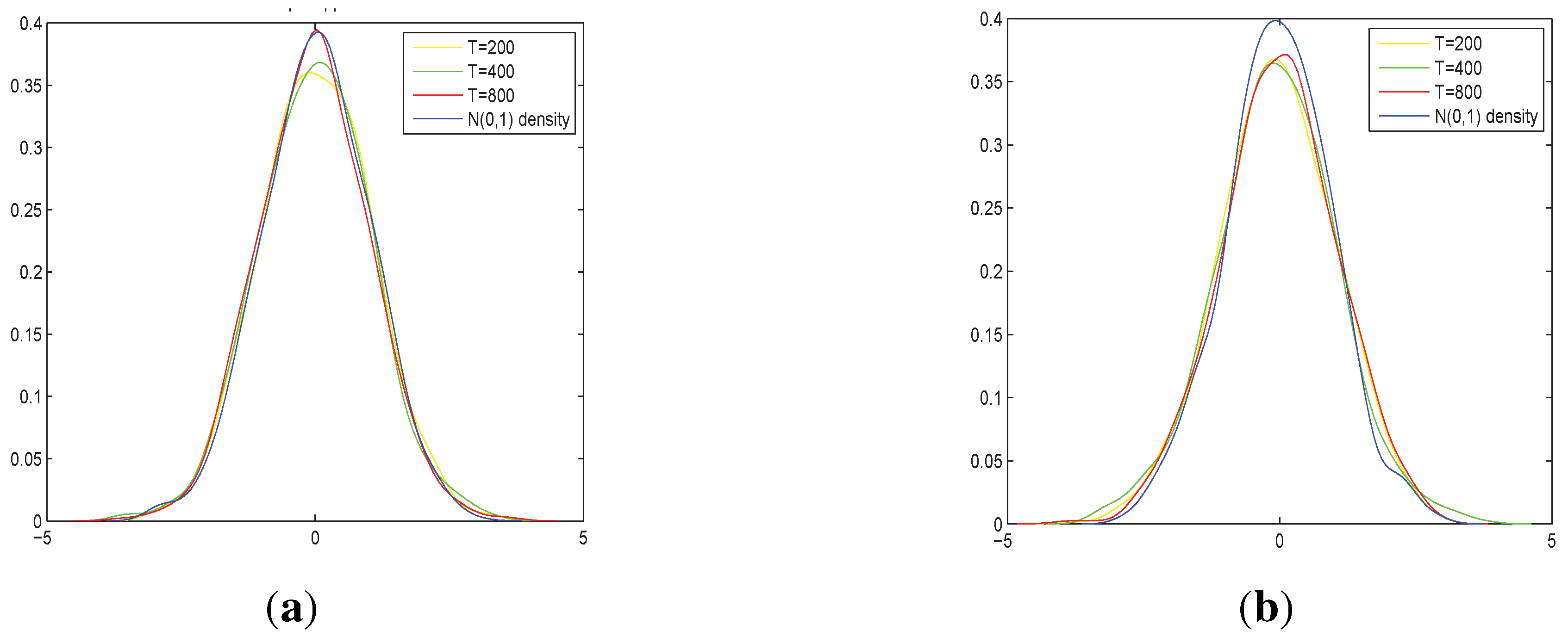
To further assess the finite sample approximation, we compare the normalized quantity in Equation (6) with the standard normal density. We compute the quantity at $[x_1{x}_2]=[00]$, the sample sizes are respectively 200, 400 and 800, the bandwidth used is $2T^{-1/12}$, the functional form is $g(x_1,x_2)=x_1\times \frac{1}{1+x_2^2}$, the variance is 1 (we use the true function of the variance rather than the estimated quantity), and the replication number is 1000.

Figure 1. In (a) we compute $\sqrt{\frac{{\sum }_{t=1}^{T}K(\frac{x_t-x}{h})}{\int K{(u)}^{2}du}}(\widehat{g}(x)-g(x))$ at point $[00]$ in each replication; in (b) we compute the normalized quantity in $\sqrt{\frac{{\sum }_{t=1}^{T}K(\frac{x_t-x}{h})}{\int K{(u)}^{2}du}}(\widehat{g}(x)-g(x))$ at the median of each replication. The number of replications is 1000.

Figure 1. In (a) we compute $\sqrt{\frac{{\sum }_{t=1}^{T}K(\frac{x_t-x}{h})}{\int K{(u)}^{2}du}}(\widehat{g}(x)-g(x))$ at point $[00]$ in each replication; in (b) we compute the normalized quantity in $\sqrt{\frac{{\sum }_{t=1}^{T}K(\frac{x_t-x}{h})}{\int K{(u)}^{2}du}}(\widehat{g}(x)-g(x))$ at the median of each replication. The number of replications is 1000.

From Figure 1a above, we can see that the approximation to normality is quite good. However, this is not always the case. For other choices of points or functional forms for evaluation, the performance may be much worse. For example, we find that when the true functional form is $g(x_1,x_2)=x_1+\frac{1}{1+x_2^2}$, there is a systematic bias in the estimation when the evaluation point is $[00]$. This phenomenon looks strange at first glance, however, it is typical in the situation when the regressors are not positive recurrent. When the regressors are null recurrent, the simulated realizations may cover very different regions of the x-axis. Hence, for a fixed evaluation point, for some replications, there may be many observations in the neighbourhood while for other replications, there may be few observations (see more discussion in [1]). Figure 1b provides the finite sample approximation of the quantity using different evaluation points for different replications, i.e., for each replication, the evaluation point is the median of the observations.

In the second model, we assume $\left\{x_t\right\}$ is a cointegrated process. Specifically, the model is:

Model 2: 

 

$$x_t=A{x}_{t-1}+u_t,$$

with $\left\{u_t\right\}\sim i.i.d.N(0,\Sigma )$ with $\Sigma =\left(\begin{array}{cc}1& 0\\ 0& 1\end{array}\right)$, $A=\left(\begin{array}{cc}3/4& 1/4\\ 1/4& 3/4\end{array}\right)$.

$$y_t=g(x_{1,t},x_{2,t})+{\epsilon }_t,$$

where $\left\{{\epsilon }_t\right\}\sim i.i.d.N(0,1)$ and is independent of $\left\{x_{1,t}\right\}$ and $\left\{x_{2,t}\right\}$. In this model, $\left\{x_t\right\}$ is 1/2-null recurrent process. We let $g(x_1,x_2)=x_1+\frac{1}{1+x_2^2}$ or $g(x_1,x_2)=x_1\times \frac{1}{1+x_2^2}$. This model falls into the category of Example 2 in Section 2. The results for Model 2 are summarized in Table 2.

Table 2. RMSEs for Model 2.

Functional Form	c	T = 200	T = 400	T = 800
	0.1	0.5098	0.3891	0.2922
	0.2	0.3853	0.2914	0.2234
$g(x_1,x_2)=x_1+\frac{1}{1+x_2^2}$	0.4	0.3038	0.2518	0.2437
	0.8	0.3481	0.3892	0.4826
	$h^{*}$	0.2941	0.2445	0.2009
	0.5	0.2513	0.1869	0.1412
	1	0.1971	0.1560	0.1323
	2	0.1890	0.1683	0.1467
$g(x_1,x_2)=x_1\times \frac{1}{1+x_2^2}$	3	0.2044	0.1773	0.1583
	4	0.2111	0.1864	0.1654
	$h^{*}$	0.1991	0.1637	0.1334

Table 2. RMSEs for Model 2.

Functional Form	c	T = 200	T = 400	T = 800
	0.1	0.5098	0.3891	0.2922
	0.2	0.3853	0.2914	0.2234
$g(x_1,x_2)=x_1+\frac{1}{1+x_2^2}$	0.4	0.3038	0.2518	0.2437
	0.8	0.3481	0.3892	0.4826
	$h^{*}$	0.2941	0.2445	0.2009
	0.5	0.2513	0.1869	0.1412
	1	0.1971	0.1560	0.1323
	2	0.1890	0.1683	0.1467
$g(x_1,x_2)=x_1\times \frac{1}{1+x_2^2}$	3	0.2044	0.1773	0.1583
	4	0.2111	0.1864	0.1654
	$h^{*}$	0.1991	0.1637	0.1334

From Table 2, we can see that for different data generating mechanism of $\left\{x_t\right\}$ or function form of g, the choice of h should be quite different. In addition, the cross validation method serves as a good choice.

Next, we consider the model where the regressors are threshold cointegrated.

Model 3: 

 

$$x_t=A{x}_{t-1}1(x_{t-1}\in D)+B{x}_{t-1}1(x_{t-1}\in D^c)+u_t,$$

with $\left\{u_t\right\}\sim i.i.d.N(0,\Sigma )$ with $\Sigma =\left(\begin{array}{cc}1& 0\\ 0& 1\end{array}\right)$, $B=\left(\begin{array}{cc}3/4& 1/8\\ 1& 1/2\end{array}\right)$, $A=\left(\begin{array}{cc}3/4& 1/4\\ 1/4& 3/4\end{array}\right)$, $D=[{\tau }_1{\tau }_2]\times [{\tau }_3{\tau }_4]=[-33]\times [-22]$ and

$$y_t=g(x_{1,t},x_{2,t})+{\epsilon }_t,$$

where $\left\{{\epsilon }_t\right\}\sim i.i.d.N(0,1)$ and is independent of $\left\{x_{1,t}\right\}$ and $\left\{x_{2,t}\right\}$. We know in this model, $\left\{x_{1,t}\right\}$ and $\left\{x_{2,t}\right\}$ are threshold cointegrated processes with different cointegrated coefficients in different regimes. According to [21], they form a bivariate 1/2-null recurrent system. We let $g(x_1,x_2)=x_1+\frac{1}{1+x_2^2}$ or $g(x_1,x_2)=x_1\times \frac{1}{1+x_2^2}$. The results for Model 3 are summarized in Table 3.

Table 3. RMSEs for Model 3.

Functional Form	c	T = 200	T = 400	T = 800
	0.1	0.8941	0.7909	0.6446
	0.5	0.4422	0.3715	0.3806
$g(x_1,x_2)=x_1+\frac{1}{1+x_2^2}$	1	0.4502	0.5221	0.6176
	2	0.7344	0.8827	1.1070
	$h^{*}$	0.4104	0.3410	0.3031
	0.5	0.4230	0.3037	0.2298
	1	0.3042	0.2625	0.2417
$g(x_1,x_2)=x_1\times \frac{1}{1+x_2^2}$	2	0.3411	0.3173	0.2874
	3	0.3732	0.3412	0.3042
	$h^{*}$	0.3175	0.2564	0.2155

Table 3. RMSEs for Model 3.

Functional Form	c	T = 200	T = 400	T = 800
	0.1	0.8941	0.7909	0.6446
	0.5	0.4422	0.3715	0.3806
$g(x_1,x_2)=x_1+\frac{1}{1+x_2^2}$	1	0.4502	0.5221	0.6176
	2	0.7344	0.8827	1.1070
	$h^{*}$	0.4104	0.3410	0.3031
	0.5	0.4230	0.3037	0.2298
	1	0.3042	0.2625	0.2417
$g(x_1,x_2)=x_1\times \frac{1}{1+x_2^2}$	2	0.3411	0.3173	0.2874
	3	0.3732	0.3412	0.3042
	$h^{*}$	0.3175	0.2564	0.2155

Our conclusion for Table 3 is same as that for Table 2.

The above three models assume the error term to be homoscedastic. In the final example, heteroscedasticity will be taken into account. The model is:

Model 4: 

 

$$\left\{x_{1,t}\right\}\sim i.i.d.N(0,1),$$

$$x_{2,t}=x_{2,t-1}+u_t,$$

with $\left\{u_t\right\}\sim i.i.d.N(0,1)$

$$y_t=g(x_{1,t},x_{2,t})+\sigma (x_{1,t},x_{2,t})e_t,$$

where $\left\{e_t\right\}\sim i.i.d.N(0,1)$ and is independent of $\left\{x_{1,t}\right\}$ and $\left\{x_{2,t}\right\}$. We let $g(x_1,x_2)=x_1+\frac{1}{1+x_2^2}$ with ${\sigma }^2(x_1,x_2)=\frac{x_1^2}{1+x_2^2}$. We estimate the conditional variance function using Equation (5) and then calculate the RMSE. In our simulation, the same bandwidth for the mean and variance functions is used.

The results for Model 4 are summarized in Table 4.

Table 4. RMSEs for Model 4.

Functions	c	T = 200	T = 400	T = 800
	1	0.2224	0.1796	0.1542
	2	0.2615	0.2352	0.2140
$g(.)$	3	0.3955	0.3674	0.3395
	4	0.5415	0.5082	0.4741
	$h^{*}$	0.2837	0.2565	0.2167
	1	0.3890	0.3196	0.2689
	2	0.3507	0.2996	0.2651
${\sigma }^2(.)$	3	0.3788	0.3369	0.2971
	4	0.4321	0.3897	0.3410
	$h^{*}$	0.7900	0.3686	0.3093

Table 4. RMSEs for Model 4.

Functions	c	T = 200	T = 400	T = 800
	1	0.2224	0.1796	0.1542
	2	0.2615	0.2352	0.2140
$g(.)$	3	0.3955	0.3674	0.3395
	4	0.5415	0.5082	0.4741
	$h^{*}$	0.2837	0.2565	0.2167
	1	0.3890	0.3196	0.2689
	2	0.3507	0.2996	0.2651
${\sigma }^2(.)$	3	0.3788	0.3369	0.2971
	4	0.4321	0.3897	0.3410
	$h^{*}$	0.7900	0.3686	0.3093

From Table 4, we can see that in general the cross validation method is not as good as in the homoscedasticity case. For some choice of fixed bandwidth, the RMSEs for mean and variance functions can be smaller. However, the cross validation is still a reasonable choice because in practice we do not know the true DGP which makes it difficult to use some pre-specified bandwidth.

In summary, we can see that the choice of bandwidth has large impact on the performance of the nonparametric estimates. The leave-one-out cross validation method is still a reasonable option for the multivariate nonparametric estimates with β-null recurrent regressor. In the empirical analysis in the next section, this method will be used.

5. Empirical Application to the Relationship of Interest Rates

In this section, we apply the proposed method to study the relationship of three interest rates: the effective Federal funds rate (FF), 3-month Treasure bill rate (TB3m) and 5-year Treasure bill rate (TB5y). The Federal Reserve (Fed) implements monetary policy by targeting the effective FF (see, e.g., [23]); the TB3m is a preeminent risk-free rate in the U.S. money market and is often used by researchers as a proxy for the risk-free asset (see, e.g., [24]), and TB5y is often used to represent the long term interest rate (see, e.g., [25]).

In the literature (cf. [23,26]), it is often argued that the interest rates move together according to the expectation hypothesis (EH) such that the Treasure bill rates are equal to market’s expectation for the FF over the term of TB rates plus a risk premium. So that according to conventional EH/montary policy views, FF “anchors" the U.S. money market. However, according to [27], the short run T-bill rate adjusts before the FF, rather than vice versa. This is possibly due to the fact that if the market anticipates changes in the FF, the T-bill rates will move in advance of the Federal funds rate. Thus, the market should have anticipated the information of the FF before its announcement. Under the same reasoning, if the short term T-bill rate contains short term information of the market, we expect that the long term T-bill rate contains long term information of the market. So that both short term and long term T-bill rates will influence the FF.

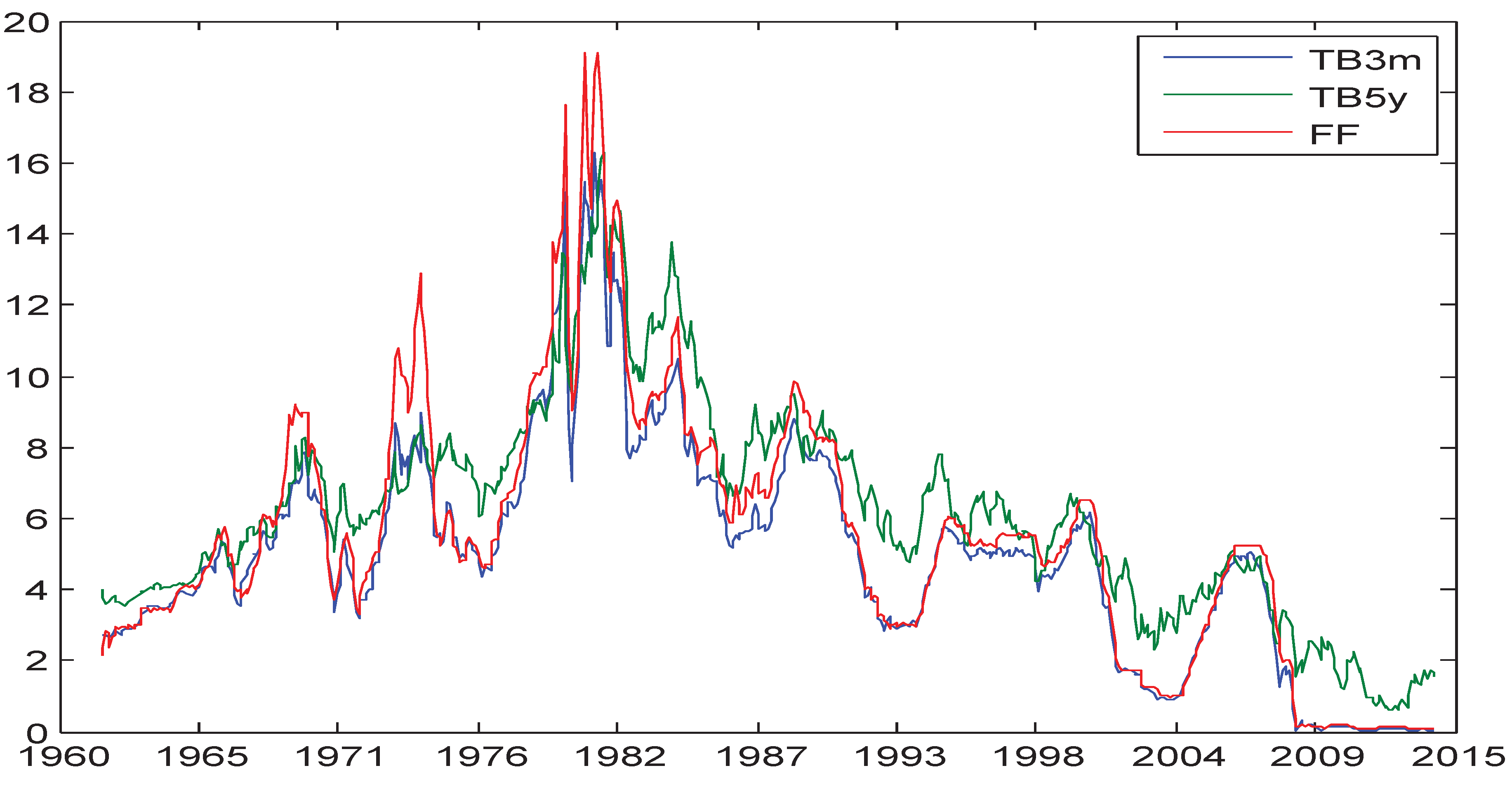
We use monthly data of FF, TB3m and TB5y from the website of the Federal Reserve Bank of St Louis. The sample period is from January 1962 to May 2014 and the sample size is 629. The ADF test suggests that all the three series contain unit roots with p-values for TB3m, TB5y and FF being respectively 0.2807, 0.3513 and 0.2648. We also perform ADF test for the interest rate differential series $\{TB3m_t-TB5y_t\}$ and the result suggests that the series is stationary with p-value being less than 0.01. This means that the short term and long term T-bill rates are cointegrated with cointegrated vector [1 −1] 3. Thus TB3m and TB5y form a 1/2-recurrent system so that we can apply the proposed method to estimate the relationship of FF with TB3m and TB5y 4.

The time series plot of the three series is shown in Figure 2.

Figure 2. Time series plot of FF, TB3m and TB5y: 1962–2014.

Figure 2. Time series plot of FF, TB3m and TB5y: 1962–2014.

From Figure 2, we can see that the three series move together. In particular, FF and TB3m seem to have a close relationship.

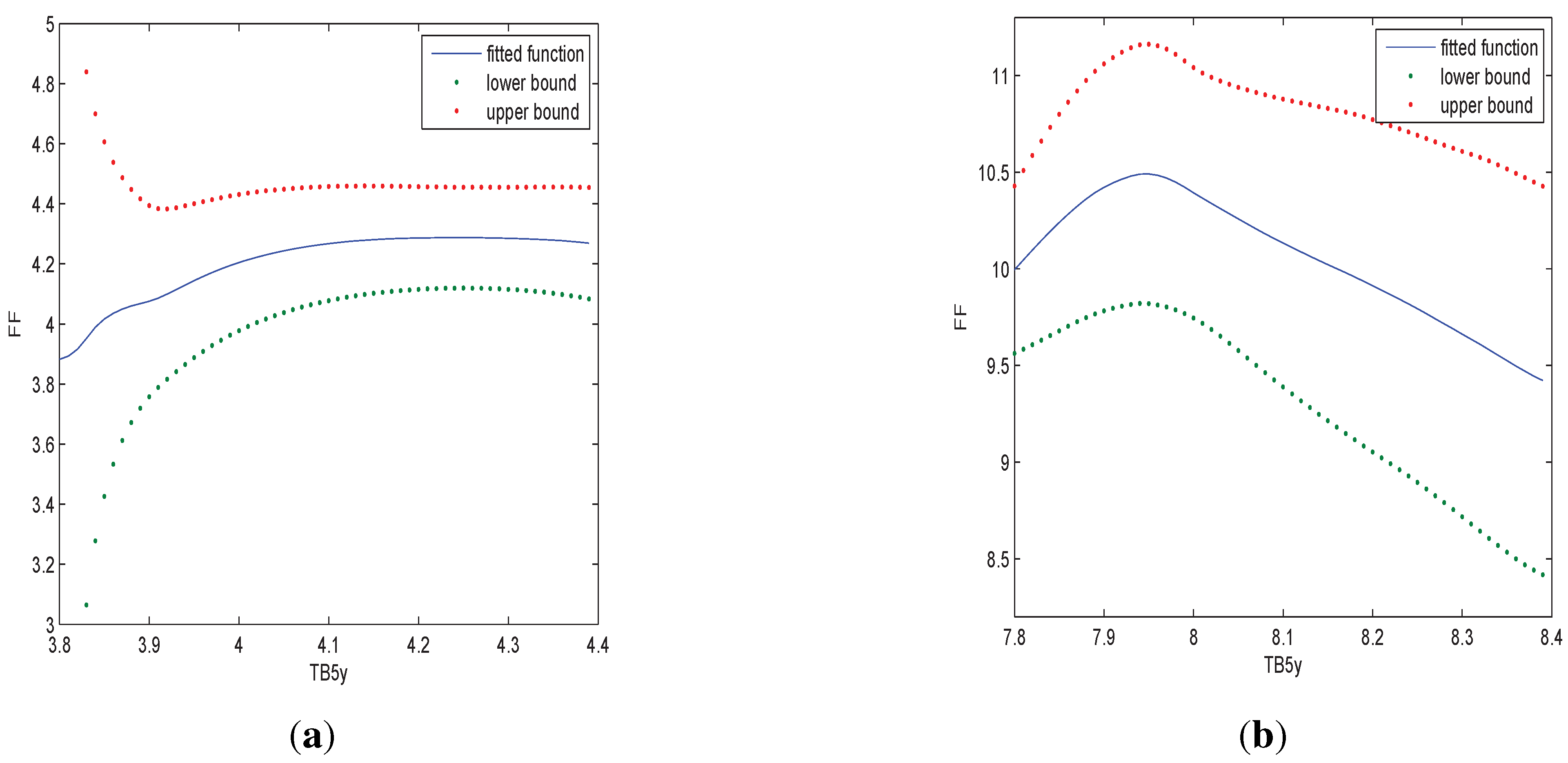
To study the relationship of the variables, in an exploratory phase we first examine the relationship of FF with TB5y when TB3m is fixed. Specifically, we plot the graph of fitted values against TB5y when TB3m is 4 or 8. Notice that because TB5y and TB3m are cointegrated, when TB3m is fixed, we can only study the relationship of FF with TB5y when TB5y is within some small regions. Otherwise, there will be insufficient observations for the nonparametric estimate5. So that when TB3m is 4, we study the relationship with TB5y within $[3.84.4]$ and when TB3m is 8, we study the relationship with TB5y within $[7.88.4]$. In addition, we can plot the $95\%$ point-wise confidence intervals according to Equation (7). The results are shown in Figure 3.

Figure 3. In (a) we estimate the relationship of FF and TB5y when TB3m is 4; in (b) we estimate the relationship of FF and TB5y when TB3m is 8.

Figure 3. In (a) we estimate the relationship of FF and TB5y when TB3m is 4; in (b) we estimate the relationship of FF and TB5y when TB3m is 8.

Figure 3 indicates that the relationship of FF with TB5y is nonlinear and the relationship is largely affected by TB3m.

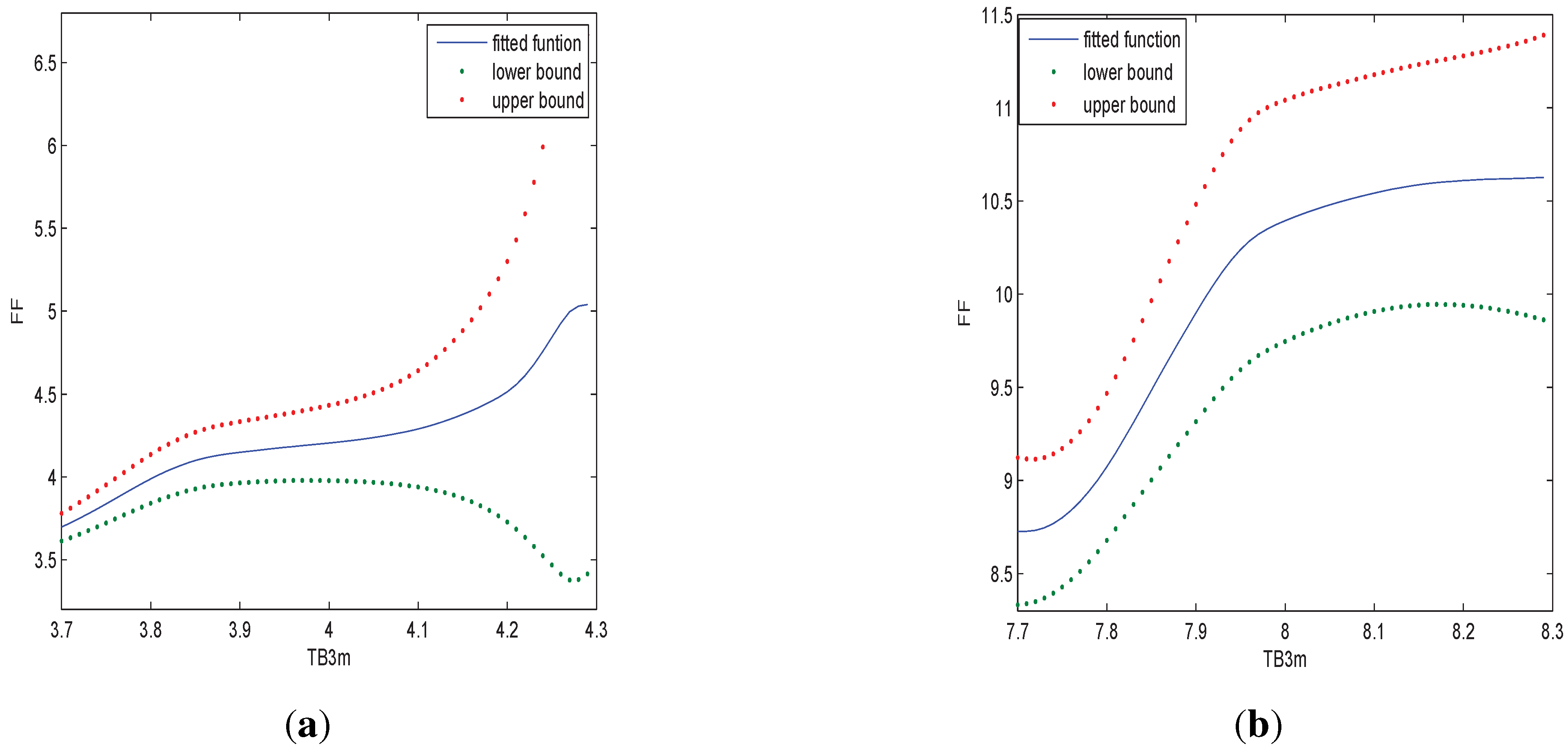
Similarly, we can examine the relationship of FF with TB3m when TB5y is fixed. When TB5y is 4, we study the relationship with TB3m within $[3.74.3]$ and when TB5y is 8, we study the relationship with TB3m within $[7.78.3]$. The results are shown in Figure 4.

Figure 4. In (a) we estimate the relationship of FF and TB3m when TB5y is 4; in (b) we estimate the relationship of FF and TB3m when TB5y is 8.

Figure 4. In (a) we estimate the relationship of FF and TB3m when TB5y is 4; in (b) we estimate the relationship of FF and TB3m when TB5y is 8.

From Figure 4, we can see that the relationship of FF with TB3m is nonlinear and different TB5y does not make large difference in the relationship.

In summary, the pairwise exploratory phase suggests that the relationship of FF and TB3m and TB5y may not be linear. The nonlinearity may be due to transaction cost as suggested by [28] or the policy interventions as suggested by [30].

Next, we estimate our model (1) by estimating g nonparametrically. We compare the in-sample mean square error of the nonparametric model with the linear model. Define the following MSE

$$MSE=\frac{1}{T}\sum _{t=1}^T{(F{F}_t-{\widehat{FF}}_t)}^2,$$

where $\widehat{FF}$ is the fitted value from the nonparametric model or the linear model (regress $FF$ on $TB3m$, $TB5y$ and a constant). The MSE for the nonparametric model is 0.0995 while the MSE for the linear model is 0.2802. It can be seen that the nonparametric model outperforms the linear model.

However, it is well known that comparison based on the in-sample performance as done above is sensitive to outliers and data mining, see, e.g., [31]. Empirical evidence of out-of-sample forecast performance is generally regarded as more trustworthy. In addition, out-of-sample forecasts can better reflect the information available to forecasters in “real time” (cf. [32]). As emphasized by [33], out-of-sample forecast is the “ultimate test of forecasting model”.

We study the out-of-sample forecasts of the nonparametric model and linear model by comparing their one-step-ahead forecasting performance. Specifically, we define the out-of-sample MSE (OMSE) as

$$OMSE=\frac{1}{m}\sum _{t=T-m+1}^T{(F{F}_t-{\widetilde{FF}}_t)}^2,$$

where ${\widetilde{FF}}_t$ is the fitted value at $(TB3m_t,TB5y_t)$ with the model estimated using the observations up to time $t-1$ 6. Furthermore, out-of-sample size m is taken to be $[1/10T]$, $[1/15T]$, $[1/20T]$, where T is the full sample size. The reason for choosing relatively small proportion of out-of-sample evaluation period is mainly due to the fact that for the nonparametric forecast, because of the nature of local estimate, a too small proportion of in-sample size may make the forecast impossible if the observation of the period we are going to forecast is an “outlier” such that we do not have enough observations in the neighborhood.

The results for the out-of-sample forecasts are reported Table 5.

Table 5. OMSE Comparison.

Model	m= [1/10 T]	m= [1/15 T]	m= [1/20 T]
Linear model	0.1018	0.0671	0.0519
Nonparametric model	0.0021	0.0022	0.0015

Table 5. OMSE Comparison.

Model	m= [1/10 T]	m= [1/15 T]	m= [1/20 T]
Linear model	0.1018	0.0671	0.0519
Nonparametric model	0.0021	0.0022	0.0015

From Table 5, we can see that the nonparametric model consistently outperforms the linear model by the out-of-sample evaluation. It is also interesting that the OMSE is smaller than the in-sample MSE. It is possible because the volatility increases with regressors (see Figure 5 below) and our out-of-sample forecasting periods are the periods where the interest rates are very low as is seen from Figure 2. The comparison of OMSE provides additional strong evidence that there exists nonlinearity in the relationship.

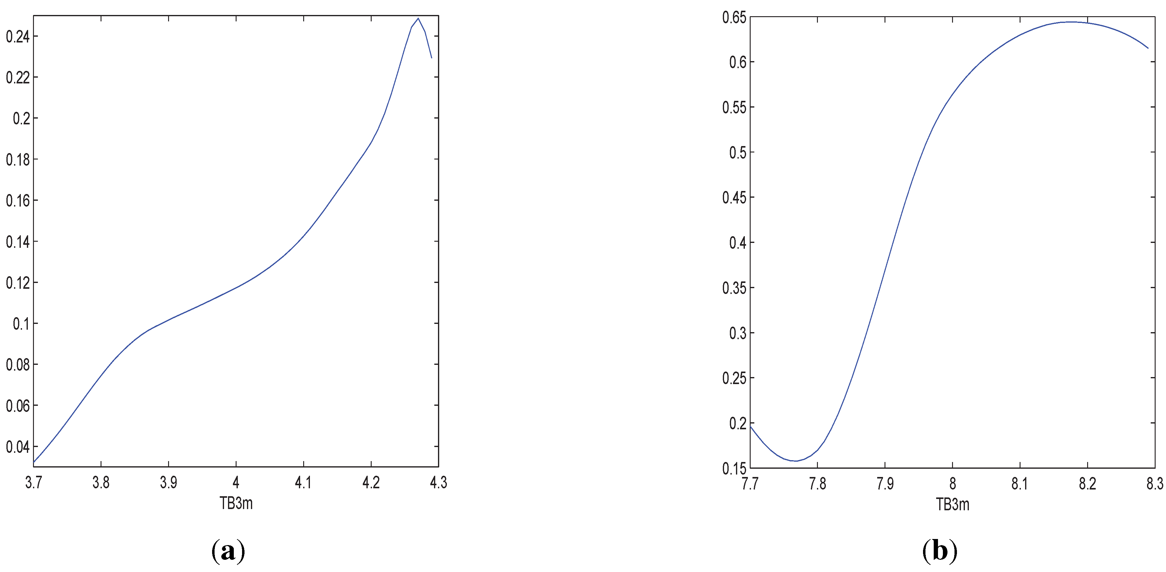
Figure 5. In (a) we estimate the shape of the variance with TB3m when TB5y = 4; in (b) we estimate the shape of the variance with TB3m when TB5y = 8.

Figure 5. In (a) we estimate the shape of the variance with TB3m when TB5y = 4; in (b) we estimate the shape of the variance with TB3m when TB5y = 8.

Similarly, we can estimate the conditional variance function using Equation (5) (with the same bandwidth as that used for the mean function estimation). Figure 5 studies the variance conditional on TB3m when TB5y is fixed. When TB5y is 4, we study shape of the variance with TB3m within $[3.74.3]$ and when TB5y is 8, we study the relationship with TB3m within $[7.78.3]$.

Figure 5 indicates that there exists conditional heteroscedasticity7. The conditional heteroscedasticity of FF is also found in [34], where a univariate model with ARCH-type (cf. [12]) volatility function is used. Chan et al. [35] study different models for the short term interest rate encompassed in the following stochastic differential equation (SDE):

$$d{r}_t=(\alpha +\beta r_t)dt+\sigma r_t^{\gamma }d{W}_t,$$

(9)

where $r_t$ is the (spot) interest rate, $W_t$ is the standard Brownian motion, α, β, σ and γ are some constants. When $\gamma =0$, Equation (9) is the Vasicek [36] model and when $\gamma =1/2$, Equation (9) is the famous Cox-Ingersoll-Ross (CIR, [37]) model. We can see that in [36], the process is conditional homoscedastic and when $\gamma \ne 0$, there exists conditional heteroscedasticity. The empirical findings of [35] suggest that γ is significantly larger than 0, so that the volatility increases with the interest rate. Our model setup is regression rather than autoregression. However, the interest rates are cointegrated and move in the same direction, so that the finding of [35] implies the volatility in our model also increases with the regressors. This is consistent with the empirical results in our paper.

6. Conclusions

In this paper, we establish the asymptotic theory of nonparametric estimation for multivariate β-null recurrent processes in presence of heteroscedasticity. The Monte Carlo simulation results suggest that the nonparametric estimator performs well using bandwidth selected by the cross validation method. The application to the relationship of Federal funds rate with short term and long term T-bill rates indicates the existence of nonlinearity.

In the current paper, the variance function estimation is not discussed in details as for the mean function estimation. This is left for future research. In empirical applications, because of different ranges of different regressors especially in this multivariate nonstationary case, different bandwidths may be used for different regressors to make the estimate more efficient (cf. [18]).