Forecast Bitcoin Volatility with Least Squares Model Averaging

Abstract

In this paper, we study forecasting problems of Bitcoin-realized volatility computed on data from the largest crypto exchange—Binance. Given the unique features of the crypto asset market, we find that conventional regression models exhibit strong model specification uncertainty. To circumvent this issue, we suggest using least squares model-averaging methods to model and forecast Bitcoin volatility. The empirical results demonstrate that least squares model-averaging methods in general outperform many other conventional regression models that ignore specification uncertainty.

1. Introduction

Bitcoin, the first and still one of the foremost applications of blockchain technology by far, was introduced early in 2008. Until the end of December 2018, the market capitalization of Bitcoin was roughly $65 billion with $3800 per token. As for the whole Bitcoin network, by the end of December 2018, there are more than 10,000 full nodes distributed across the world and roughly $2.5 billion of value transacted on the main network. With the growth of the Bitcoin market, many investors are starting to view it as an emerging new asset class. In September 2015, the Commodity Futures Trading Commission (CFTC) in the United States officially designated Bitcoin as a commodity. Improved measures of Bitcoin volatility enable us to better gauge the current level of volatility and to understand its dynamics. Most importantly, Bitcoin volatility is now directly tradable,1 which accredits the importance of Bitcoin volatility forecasting.

How to model and predict the volatility of financial assets is an interesting topic in risk management. Traditional approaches employ parametric models such as the generalized autoregressive conditional heteroskedasticity (GARCH) or stochastic volatility models. Recently a new approach to modeling volatility dynamics has relied on improved measures of ex post volatility composed from high-frequency intraday data. This new measure is called realized volatility (RV), which possesses a slowly decaying autocorrelation function, sometimes known as long-memory.2 Various models have been proposed to capture stylized facts of realized volatility series, such as the fractionally integrated autoregressive moving average (ARFIMA) models3 used in Andersen et al. (2001b) and the heterogeneous autoregressive (HAR) model proposed by Corsi (2009). Compared with the ARFIMA model, the HAR model soon gained popularity because of its computational simplicity (e.g., ordinary least squares) and excellent out-of-sample performance.4

The HAR model can provide an intuitive economic interpretation that agents with three frequencies of trading (daily, weekly, and monthly) perceive and respond to, which changes the corresponding components of volatility.5 Nevertheless, the suitability of such a specification is not subject to enough verification. Craioveanu and Hillebrand (2012) employed a parallel computing method to investigate all the possible combinations of lags in the additive model. Others tested the validity of the lag structure in the conventional HAR model from a model selection perspective; see, e.g., Audrino et al. (2015,2016); and Audrino et al. (2016), among others. While the lag terms in the HAR model survive the tests based on the least absolute shrinkage and selection operator (LASSO) and the adaptive LASSO (Audrino et al. 2015; Audrino and Knaus 2016) only in the case of simulated data by the HAR model, there is strong evidence in Audrino et al. (2016) that casts some doubts on the fixed choice of aggregation frequencies in the HAR model. In particular, Audrino et al. (2016) found that a conventional fixed lag structure was not statistically sustained by the group LASSO estimates for certain individual stocks in an unstable market environment such as the 2007–2009 crisis. They addressed the above issue with a proposed flexible HAR model, built dynamically from the group LASSO estimates.

The above conclusions may or may not hold in Bitcoin volatility forecasting considering the unique features of the crypto asset market. To tackle this question from a different angle, we consider the forecast implication of a flexible lag structure generated by the least squares model-averaging method. Unlike the model selection approach that picks only one winning model out of a pool of candidate models, model averaging calculates the weighted average of a group of candidate models. Barnard (1963) first discussed the concept of “model combination” in a paper studying airline passenger data. Buckland et al. (1997) suggested using the exponential Akaike information criterion (AIC) estimates as the model weights and proposed the model averaged AIC. There exists many other averaging-type approaches that provide a means to tackle model uncertainty, for instance, the Bayesian model-averaging method discussed in length in Hoeting et al. (1999), the weighted-average least squares method by Magnus et al. (2010), and the random forest method by Breiman (2001), among others.

The performance of the model-averaging method heavily relies on the weights chosen for the estimation process. In a pioneering study, Hansen (2007) proposed the Mallows model averaging (MMA) method that is asymptotically optimal in the sense of achieving the lowest possible mean squared errors. Wan et al. (2010) completed the theoretical foundation of the MMA. Extensions of the MMA that allow possible structural breaks, near unit root, and heteroskedasticity can be found in Hansen (2009,2010), and Hansen and Racine (2012), respectively. Xie (2015) proposed the prediction model averaging (PMA) method. Zhao et al. (2016) extended the PMA method to allow for heteroskedastic error terms (HPMA). Liu and Okui (2013) also proposed a heteroskedasticity-robust Mallows’ $C_p$ model-averaging method (HRCP).

There is a growing literature on solving the model uncertainty issue in volatility forecasting with least squares model averaging. Lehrer et al. (2018) proposed the model averaging HAR (MAHAR) method that optimally averages the forecasts of HAR models with different lag indexes. Qiu et al. (2019) showed that the above method can be extended to a more complicated HAR model with estimators of the variation of positive and negative returns (semi-variance components). Besides the above methods, we consider the approach designed by Qiu and Xie (2018), who proposed the heteroskedasticity-robust model averaging HAR method (H-MAHAR) that mainly applies the HPMA as the core model averaging estimator to exchange rate volatility. As a complement to the HPMA, we also include the jackknife model averaging (JMA) and the heteroskedasticity robust $C_p$ (HRCP) model averaging estimators as companion methods in this paper.

In the empirical exercise, we consider a series of estimators including 9 conventional regression methods, 1 LASSO method, and 4 model-averaging methods to model and forecast the realized variance of Bitcoin prices. We show that the model-averaging methods that account for model uncertainty generally outperform the conventional regressions and the model-selection-based LASSO method. Moreover, the heteroskedasticity-robust methods tend to perform relatively better. Compared with non-model-averaging methods, the H-MAHAR method yields the highest forecasting accuracy in most of the exercises. The improvement that H-MAHAR provides is statistically significant at the 5% level, as confirmed by the Giacomini–White test (Giacomini and White 2006).

The reminder of the paper is arranged as follows. Section 2 provides a more detailed overview of existing HAR strategies. Section 3 discusses the way to model uncertainty under heteroskedasticity using least squares model averaging. Section 4 describes the data. Section 5 presents the empirical results, where we compared 14 methods in rolling window exercises. In all cases, model-averaging methods tended to have the dominating performance. To examine the robustness of the results, we tried different experimental settings in Section 6. Section 7 concludes this paper.

2. Prior HAR-Type Strategies to Forecast Volatility

Following Andersen and Bollerslev (1998), we estimate daily RV at day t (${\mathrm{RV}}_t$) by summing the corresponding M equally spaced intra-daily squared returns $r_{t,j}$. Here, the subscript t indexes day t and j indicates the time within day t,

$${\mathrm{RV}}_t\equiv \sum _{j=1}^M{r}_{t,j}^2$$

(1)

where $t=1,2,\dots ,T$, $j=1,2,\dots ,M$, and $r_{t,j}$ define continuously compounded high-frequency returns by differing log-prices $p_{t,j}$ ($r_{t,j}=p_{t,j}-p_{t,j-1}$).

Among the RV models, the HAR model proposed by Corsi (2009) is quite prevalent. Not only is this because the HAR model accurately approximates the long-memory and multiscaling properties of RV but also this is very easy to implement in practice. The standard HAR model in Corsi (2009) postulates that the h-step-ahead daily ${\mathrm{RV}}_{t+h}$ can be described by

$${\mathrm{RV}}_{t+h}={\beta }_0+{\beta }_d{\mathrm{RV}}_t^{\left(1\right)}+{\beta }_w{\mathrm{RV}}_t^{\left(5\right)}+{\beta }_m{\mathrm{RV}}_t^{\left(22\right)}+e_{t+h},$$

(2)

where the explanatory variables can take the general form of ${\mathrm{RV}}_t^{\left(l\right)}$. ${\mathrm{RV}}_t^{\left(l\right)}$ is defined by

$${\mathrm{RV}}_t^{\left(l\right)}\equiv l^{-1}\sum _{s=1}^l{\mathrm{RV}}_{t-s}$$

(3)

where l is the period averages of daily RV, $\beta$ is the coefficients, and ${\left\{e_t\right\}}_t$ is a zero mean innovation process. The standard HAR model in Equation (2) is pinned down by some vector of lag index $\mathit{l}=[1,5,22]$.

Andersen et al. (2007) extended the standard HAR model two ways. First, they added the daily jump component ${\mathrm{J}}_t$ to Equation (2) to explicitly capture its impacts. The extended model is denoted the HAR-J model:

$${\mathrm{RV}}_{t+h}={\beta }_0+{\beta }_d{\mathrm{RV}}_t^{\left(1\right)}+{\beta }_w{\mathrm{RV}}_t^{\left(5\right)}+{\beta }_m{\mathrm{RV}}_t^{\left(22\right)}+{\beta }^j{\mathrm{J}}_t+e_{t+h},$$

(4)

where the empirical measurement of the squared jumps is ${\mathrm{J}}_t=max({\mathrm{RV}}_t-{\mathrm{BPV}}_t,0)$ and the standardized realized bipower variation (BPV) is defined as

$${\mathrm{BPV}}_t\equiv {(2/\pi )}^{-1}\sum _{j=2}^M|r_{t,j-1}||r_{t,j}|.$$

Second, through a decomposition of RV into the continuous sample path and the jump component based on the $Z_{1,t}$ statistic, Andersen et al. (2007) reconstructed the HAR-J model by explicitly incorporating the two types of volatility components mentioned above. The $Z_{1,t}$ statistic identifies the “significant” jumps ${CJ}_t$ and the continuous sample path components ${CSP}_t$ respectively as

$$\begin{array}{ccc}\hfill {\mathrm{CSP}}_t& \equiv & \mathbb{I}(Z_t\le {\mathsf{\Phi }}_{\alpha })·{\mathrm{RV}}_t+\mathbb{I}(Z_t\le {\mathsf{\Phi }}_{\alpha })·{\mathrm{BPV}}_t,\hfill \\ \hfill {\mathrm{CJ}}_t& =& \mathbb{I}(Z_t>{\mathsf{\Phi }}_{\alpha })·max({\mathrm{RV}}_t-{\mathrm{BPV}}_t,0),\hfill \end{array}$$

where $Z_t$ is the ratio statistic in Huang and Tauchen (2005)6 and ${\mathsf{\Phi }}_{\alpha }$ is the cumulative distribution function (CDF) of a standard Gaussian distribution with an $\alpha$ level of significance. The daily, weekly, and monthly average components of CSP${}_t$ and CJ${}_t$ are then constructed in the same manner as ${\mathrm{RV}}^{\left(l\right)}$ in Equation (3). The model specification for the continuous HAR-J, in other words, the HAR-CJ, is given by

$${\mathrm{RV}}_{t+h}={\beta }_0+{\beta }_d^c{\mathrm{CSP}}_t^{\left(1\right)}+{\beta }_w^c{\mathrm{CSP}}_t^{\left(5\right)}+{\beta }_m^c{\mathrm{CSP}}_t^{\left(22\right)}+{\beta }_d^j{\mathrm{CJ}}_t^{\left(1\right)}+{\beta }_w^j{\mathrm{CJ}}_t^{\left(5\right)}+{\beta }_m^j{\mathrm{CJ}}_t^{\left(22\right)}+e_{t+h}.$$

(5)

Note the HAR-CJ model explicitly controls for the weekly and monthly effects of continuous jumps through the CJ${}_t^{\left(1\right)}$, CJ${}_t^{\left(5\right)}$, and CJ${}_t^{\left(22\right)}$ terms, whereas the HAR-J model consists of only one aggregate jump term J${}_t$. Thus, the HAR-J model can be regarded as a special and restrictive case of the HAR-CJ model for ${\beta }_d={\beta }_d^c+{\beta }_d^j$, ${\beta }^j={\beta }_d^j$, ${\beta }_w={\beta }_w^c+{\beta }_w^j$, and ${\beta }_m={\beta }_m^c+{\beta }_m^j$.

To capture the role of the “leverage effect” in predicting volatility dynamics, Patton and Sheppard (2015) developed a group of models using signed realized measures. The first model, denoted as HAR-RS-I, decomposes the daily RV in the standard HAR model (Equation (2)) into two asymmetric semi-variances: ${\mathrm{RS}}_t^{+}$ and ${\mathrm{RS}}_t^{-}$.

$${\mathrm{RV}}_{t+h}={\beta }_0+{\beta }_d^{+}{\mathrm{RS}}_t^{+}+{\beta }_d^{-}{\mathrm{RS}}_t^{-}+{\beta }_w{\mathrm{RV}}_t^{\left(5\right)}+{\beta }_m{\mathrm{RV}}_t^{\left(22\right)}+e_{t+h},$$

(6)

where ${\mathrm{RS}}_t^{-}={\sum }_{j=1}^M{r}_{t,j}^2·\mathbb{I}(r_{t,j}<0)$ and ${\mathrm{RS}}_t^{+}={\sum }_{j=1}^M{r}_{t,j}^2·\mathbb{I}(r_{t,j}>0)$. To verify whether the realized semi-variances add something beyond the classical leverage effect, Patton and Sheppard (2015) augmented the HAR-RS-I model with a term interacting the lagged RV with an indicator for negative lagged daily returns ${\mathrm{RV}}_t^{\left(1\right)}·\mathbb{I}(r_t<0)$. The second model in Equation (7) is named HAR-RS-II.

$${\mathrm{RV}}_{t+h}={\beta }_0+{\beta }_1{\mathrm{RV}}_t^{\left(1\right)}·\mathbb{I}(r_t<0)+{\beta }_d^{+}{\mathrm{RS}}_t^{+}+{\beta }_d^{-}{\mathrm{RS}}_t^{-}+{\beta }_w{\mathrm{RV}}_t^{\left(5\right)}+{\beta }_m{\mathrm{RV}}_t^{\left(22\right)}+e_{t+h},$$

(7)

where ${\mathrm{RV}}_t^{\left(1\right)}·\mathbb{I}(r_t<0)$ is designed to capture the effect of negative daily returns. As in the HAR-CJ model, the third and fourth models in Patton and Sheppard (2015), denoted as HAR-SJ-I and HAR-SJ-II respectively, disentangle the signed jump variations and the BPV from the volatility process.

$$\begin{array}{ccc}\hfill {\mathrm{RV}}_{t+h}& =& {\beta }_0+{\beta }_d^j{\mathrm{SJ}}_t+{\beta }_d^{bpv}{\mathrm{BPV}}_t+{\beta }_w{\mathrm{RV}}_t^{\left(5\right)}+{\beta }_m{\mathrm{RV}}_t^{\left(22\right)}+e_{t+h},\hfill \end{array}$$

(8)

$$\begin{array}{ccc}\hfill {\mathrm{RV}}_{t+h}& =& {\beta }_0+{\beta }_d^{j-}{\mathrm{SJ}}_t^{-}+{\beta }_d^{j+}{\mathrm{SJ}}_t^{+}+{\beta }_d^{bpv}{\mathrm{BPV}}_t+{\beta }_w{\mathrm{RV}}_t^{\left(5\right)}+{\beta }_m{\mathrm{RV}}_t^{\left(22\right)}+e_{t+h},\hfill \end{array}$$

(9)

where ${\mathrm{SJ}}_t={\mathrm{RS}}_t^{+}-{\mathrm{RS}}_t^{-}$, ${\mathrm{SJ}}_t^{+}={\mathrm{SJ}}_t·\mathbb{I}({\mathrm{SJ}}_t>0)$, and ${\mathrm{SJ}}_t^{-}={\mathrm{SJ}}_t·\mathbb{I}({\mathrm{SJ}}_t<0)$. The HAR-SJ-II model extends the HAR-SJ-I model by distinguishing the effect of a positive jump variation from that of a negative jump variation.

3. Model Uncertainty

It has been a tradition for the past literature to assume the lag structure of the HAR model to be $\mathit{l}=[1,5,22]$, which mimics the daily, weekly, and monthly traders in traditional financial markets that only open on workdays. On the other hand, given the 24/7 nonstop nature of bitcoin trading, it may not be appropriate to set the lag index at $[1,5,22]$. An initial guess for the lag index would be $\mathit{l}=[1,7,30]$ that represents the tradition of daily, weekly, and monthly averages. However, the suitability of such a specification is subject to a statistical investigation, which is likely to cause evident model uncertainty.

Suppose the dependent variable is $\mathit{y}={[{\mathrm{RV}}_1,\dots ,{\mathrm{RV}}_T]}^{\top }$ and the explanatory variable is $\mathit{X}={[{\mathit{x}}_1,\dots ,{\mathit{x}}_T]}^{\top }$,7 where the specification of ${\mathit{x}}_t$ takes the general form of the HAR model

$${\mathit{x}}_t=\left[1,{\mathrm{RV}}_{t-h}^{\left(l_1\right)},{\mathrm{RV}}_{t-h}^{\left(l_2\right)},\dots ,{\mathrm{RV}}_{t-h}^{\left(l_p\right)}\right].$$

(10)

Here, we do not restrict the lag index $\mathit{l}=[l_1,l_2,\dots ,l_p]$ to be $[1,5,22]$. Instead, we acknowledge the specification uncertainty in $\mathit{l}$ and consider a group of M candidate models to approximate the true data generating process. Following an usual approach in the model averaging literature, the set of M candidate models is constructed by taking a full permutation of all the lags from ${\mathrm{RV}}_{t-h}^{\left(l_1\right)}$ to ${\mathrm{RV}}_{t-h}^{\left(l_p\right)}$ (${\mathrm{RV}}_{t-h}^{\left(l_1\right)},\dots ,{\mathrm{RV}}_{t-h}^{\left(l_p\right)}$ and $[l_1,\dots ,l_p]=[1,\dots ,30]$). The maximum lag order $l_p$ is chosen as 30. In this way, there are distinct model weights assigned to each HAR-type model with different lag combinations. Moreover, as the underlying data sets vary, this will alter the relevant model weights, which effectively makes the method dynamic and data-driven.

Note that the model averaging estimator with pre-screened candidate models is implemented in this paper, since keeping the total number of candidate models manageable or slowing its convergence to infinity is a necessary condition to maintain the asymptotic optimality of least square model averaging estimators. However, in the context of the HAR model with a maximum lag order of $l_p$, we could end up with $2^{l_p}$ candidate models and the number of potential models grows exponentially with $l_p$. To solve this issue, we first apply the model screening method, for example, the adaptive regression by mixing with the model selection (ARMS) approach by Yuan and Yang (2005) or the hetero-robust model screening (HRMS) approach by Xie (2017). Both methods shrink the number of potential models by specifying model selection criteria before model averaging to an appropriate degree.

The true model is presumed to be

$$\mathit{y}=\mathit{\mu }+\mathit{e},$$

(11)

where $\mathit{y}={[y_1,\dots ,y_T]}^{\top }$, $\mathit{\mu }={[{\mu }_1,\dots ,{\mu }_T]}^{\top }$, and $\mathit{e}={[e_1,\dots ,e_T]}^{\top }$. ${\mu }_t$ can be considered the conditional mean in the period t, ${\mu }_t=\mathbb{E}\left(y_t\right|y_{t-h},y_{t-h-1},\dots )$, and the error term $e_t$ has the zero conditional mean $\mathbb{E}\left(e_t\right|y_{t-h},y_{t-h-1},\dots )=0$. Note that the error term $\mathit{e}$ is assumed to be heteroskedastic such that $\mathbb{E}\left(e_t^2\right|{\mathit{x}}_t)={\sigma }_t^2$, which reflects a more realistic characterization of the realized volatility for a wide class of financial assets. In addition, we also hypothesize that $\mathit{e}$ is not serially correlated and $\mathbb{E}\left({\mathit{e}}^{\top }\mathit{e}\right|\mathit{X})=\mathsf{\Omega }=\mathrm{diag}\{{\sigma }_1^2,\dots ,{\sigma }_T^2\}$.8 Let the mth candidate model be

$$\mathit{y}={\mathit{X}}^m{\mathit{\beta }}^m+{\mathit{e}}^m,$$

where ${\mathit{X}}^m$ are subsets of columns of $\mathit{X}$. With ${\mathit{X}}^m$ at hand, ${\mathit{\beta }}^m$ can be estimated by ${\widehat{\mathit{\beta }}}^m={\left({{\mathit{X}}^m}^{\top }{\mathit{X}}^m\right)}^{-1}{{\mathit{X}}^m}^{\top }\mathit{y}$, and thus, $\mathit{\mu }$ is estimated by

$${\widehat{\mathit{\mu }}}^m={\mathit{X}}^m{\widehat{\mathit{\beta }}}^m={\mathit{X}}^m{\left({{\mathit{X}}^m}^{\top }{\mathit{X}}^m\right)}^{-1}{{\mathit{X}}^m}^{\top }\mathit{y}={\mathit{P}}^m\mathit{y},$$

where ${\mathit{P}}^m$ is a projection matrix for the model m. Extending from Hansen (2008), the optimal mean-square h-period ahead forecast is the conditional mean ${\mu }_{T+h}$. Therefore, the least-squares forecast of $y_{T+h}$ from the mth approximation model is then ${\widehat{y}}_{T+h}^m={\widehat{\mu }}_{T+h}^m={{\mathit{x}}_{T+h}^m}^{\top }{\widehat{\mathit{\beta }}}^m$. Note that by the definition of Equation (10), ${\mathit{x}}_{T+h}^m$ is observable in period t.

We obtain the forecasts of $y_{T+h}$ from all approximation models and define the vector of forecasts ${\widehat{\mathit{y}}}_{T+h}$

$${\widehat{\mathit{y}}}_{T+h}\equiv {\left[{\widehat{y}}_{T+h}^1,{\widehat{y}}_{T+h}^2,\cdots ,{\widehat{y}}_{T+h}^M\right]}^{\top }.$$

(12)

The model averaging forecast is simply the weighted average of ${\widehat{\mathit{y}}}_{T+h}$ such that

$${\widehat{y}}_{T+h}\left(\mathit{w}\right)\equiv {\mathit{w}}^{\top }{\widehat{\mathit{y}}}_{T+h}=\sum _{m=1}^M{w}^m{\widehat{y}}_{T+h}^m,$$

where $\mathit{w}={\left[w^1,\dots ,w^M\right]}^{\top }$ is a weight vector in the unit simplex in ${\mathbb{R}}^M$

$$\mathcal{H}\equiv \left\{\mathit{w}\in {[0,1]}^M:\sum _{m=1}^M{w}^m=1\right\}.$$

The performance of model averaging forecast crucially depends on the weight vector $\mathit{w}$. The model averaging estimator of the conditional mean is then given by

$$\widehat{\mathit{\mu }}\left(\mathit{w}\right)\equiv \mathit{P}\left(\mathit{w}\right)\mathit{y},$$

(13)

where $\mathit{P}\left(\mathit{w}\right)\equiv {\sum }_{m=1}^M{w}^m{\mathit{P}}^m$ is the averaged projection matrix. The H-MAHAR method is the heteroskedasticity-robust version of the model averaging HAR (MAHAR) method proposed by Lehrer et al. (2018). The MAHAR criterion function is defined as follows:

$$\mathrm{MAHAR}\left(\mathit{w}\right)={\left(\mathit{y}-\widehat{\mathit{\mu }}\left(\mathit{w}\right)\right)}^{\top }\left(\mathit{y}-\widehat{\mathit{\mu }}\left(\mathit{w}\right)\right)\left(\frac{T+k\left(\mathit{w}\right)}{T-k\left(\mathit{w}\right)}\right),$$

(14)

where $k\left(\mathit{w}\right)\equiv {\sum }_{m=1}^M{w}^m{k}^m$ is the effective number of parameters and $k^m$ is the number of regressors in the model m. We estimate the MAHAR weight estimator by minimizing the MAHAR criterion function under the restriction of $\mathit{w}\in \mathcal{H}$.

Like most model selection and model averaging criteria, the H-MAHAR criterion balances between the fit and the complexity of a model:

$$\mathrm{H}-\mathrm{MAHAR}\left(\mathit{w}\right)={\left(\mathit{y}-\widehat{\mathit{\mu }}\left(\mathit{w}\right)\right)}^{\top }\left(\mathit{y}-\widehat{\mathit{\mu }}\left(\mathit{w}\right)\right)+2\mathrm{tr}\left(\mathit{P}\left(\mathit{w}\right)\widehat{\mathsf{\Omega }}\left(\mathit{w}\right)\right),$$

(15)

where $\widehat{\mathsf{\Omega }}\left(\mathit{w}\right)\equiv \mathrm{diag}\{{\widehat{e}}_1^2\left(\mathit{w}\right),\dots ,{\widehat{e}}_T^2\left(\mathit{w}\right)\}$ is the averaged estimate of the $\mathsf{\Omega }$ matrix using model averaging residuals $\widehat{\mathit{e}}\left(\mathit{w}\right)={[{\widehat{e}}_1^2\left(\mathit{w}\right),\dots ,{\widehat{e}}_T^2\left(\mathit{w}\right)]}^{\top }=\mathit{y}-\widehat{\mathit{\mu }}\left(\mathit{w}\right)$.

The criterion in Equation (15) can be implemented to compute the empirical weight vector $\widehat{\mathit{w}}$ through

$$\widehat{\mathit{w}}=\underset{\mathit{w}\in \mathcal{H}}{argmin}\mathrm{H}-\mathrm{MAHAR}\left(\mathit{w}\right).$$

Therefore, we obtain the model averaging forecast of $y_{T+h}$ following ${\widehat{y}}_{T+h}\left(\widehat{\mathit{w}}\right)={\widehat{\mathit{w}}}^{\top }{\widehat{\mathit{y}}}_{T+h}$. Note that the H-MAHAR estimator can be considered an extension to the model averaging with averaging covariance matrix (MAACM) estimator of Zhao et al. (2016) under the HAR framework, whereas the original MAACM estimator assumes no dynamic model structures.

Another heteroskedasticity-robust model-averaging method is the JMA estimator by Hansen and Racine (2012). The original JMA deals with cross-sectional data. Zhang et al. (2013) proved the asymptotic optimality of the JMA estimator under a dependent time-series. The JMA estimator is also known as leave-one-out cross-validation model averaging. As its name indicates, the JMA requires the use of jackknife residuals for the average estimator. The jackknife residual vector for model m can be conveniently expressed as ${{\widehat{\mathit{e}}}^m}_{\mathit{J}}={\mathit{D}}^m{\widehat{\mathit{e}}}^m$, where ${\widehat{\mathit{e}}}^m$ is the least squares residual vector and ${\mathit{D}}^m$ is the $n\times n$ diagonal matrix with the ith diagonal element equal to ${(1-h_i^m)}^{-1}$. The term $h_i^m$ is the ith diagonal element of the projection matrix ${\mathit{P}}^m$. Define an $n\times M$ matrix with all the jackknife residuals, in which ${\widehat{\mathit{E}}}_{\mathit{J}}=\left[{{\widehat{\mathit{e}}}^{\left(1\right)}}_{\mathit{J}},\dots ,{{\widehat{\mathit{e}}}^{\left(M\right)}}_{\mathit{J}}\right].$ The least squares cross-validation criterion for the JMA is simply

$${\mathrm{JMA}}_n\left(\mathit{w}\right)=\frac{1}{n}{\mathit{w}}^{\top }{\widehat{\mathit{E}}}_{\mathit{J}}^{\top }{\widehat{\mathit{E}}}_{\mathit{J}}^{}\mathit{w}$$

with model weights $\mathit{w}$ estimated through $\widehat{\mathit{w}}={\mathrm{argmin}}_{\mathit{w}\in \mathcal{H}}{\mathrm{JMA}}_n\left(\mathit{w}\right)$.

Liu and Okui (2013) adopted the same model setup to propose the HRCP model averaging estimator for linear regression models with heteroskedastic errors. They demonstrated the asymptotic optimality of the HRCP estimator when the error term exhibits heteroskedasticity. They proposed estimating the model weights by the following feasible HRCP criterion:

$$\mathrm{HRCP}\left(\mathit{w}\right)={∥\mathit{y}-\mathit{P}\left(\mathit{w}\right)\mathit{y}∥}^2+2\sum _{i=1}^n{\widehat{\mathit{e}}}_i^2{p}_{ii}\left(\mathit{w}\right)$$

(16)

with $\widehat{\mathit{w}}=\underset{\mathit{w}\in \mathcal{H}}{argmin}\mathrm{HRCP}\left(\mathit{w}\right)$. Obtaining $\mathit{w}$ by minimizing Equation (16) under the condition $\mathit{w}\in \mathcal{H}$ is a quadratic optimization process.

Equation (16) includes a preliminary estimate ${\widehat{e}}_i$ that must be obtained prior to estimation. Liu and Okui (2013) discussed several ways to obtain ${\widehat{e}}_i$ in practice. When the models are nested, Liu and Okui (2013) suggested using the residuals from the largest model. When the models are non-nested, they recommended building a model that contains all the regressors in the potential models and taking the corresponding predicted residuals. In addition, a degree-of-freedom correction on ${\widehat{e}}_i$ is reccomended to improve finite-sample properties. For example, when the mth model is chosen to obtain ${\widehat{e}}_i$, we may use

$$\widehat{\mathit{e}}=\sqrt{n/(n-k^m)}(\mathit{I}-{\mathit{P}}^m)\mathit{y}$$

instead of $(\mathit{I}-{\mathit{P}}^m)\mathit{y}$ to generate the preliminary estimate ${\widehat{e}}_i$.

4. Data Description

Binance was founded in September 2017 and is now the largest crypto exchange around the world. Since the Bitcoin to U.S. dollar (BTC/USD) price data on Binance has only recently become available, we use the data from 1 January 2018 to 20 December 2018 for this exercise. The total number of daily observations is 352. We estimate the daily RV using Equation (1) at the 5-min interval.

The evolution of the RV data over this period is plotted by the solid line in the upper panel of Figure 1, whereas the horizontal axis represents the date and the vertical axis on the left-hand side stands for RV. Besides RV, the price of BTC/USD is also depicted by the dashed line with the vertical axis on the right-hand- ide representing the price. We also list the corresponding daily trading volume in the lower panel of Figure 1. As seen in Figure 1, the dynamics of the RV follow the movements of price and volume: the RV increases as the price changes dramatically, which is usually accompanied by a noticeable peak in the trading volume.

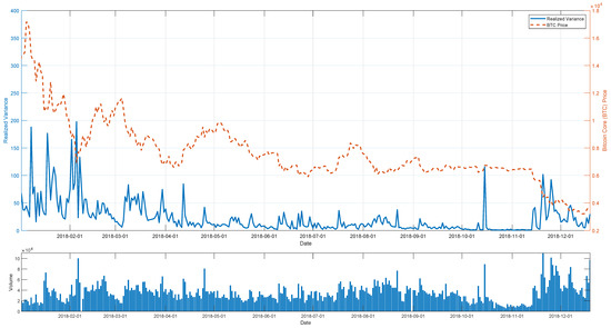
Figure 1. BTC/USD price, realized variance, and volume on Binance.

Table 1 presents summary statistics for the data and p-values of both the Jarque–Bera (JB) test for normality and of the Augmented Dickey–Fuller (ADF) tests for unit root. Note that, for the JB and ADF test statistics that are outside tabulated critical values, we report the maximum (0.999) or minimum (0.001) p-values. In Table 1, we consider the first half, the second half, and full samples in columns 2–4, respectively. Each of the series exhibits tremendous variability and a large range across the respective sample period. Furthermore, none of the series are normally distributed or nonstationary at the 5% level.

Table 1. Descriptive statistics of the BTC/USD RV.

Statistics	First Half	Second Half	Full Sample
Mean	32.4200	12.3319	22.3760
Median	21.9565	6.4271	11.8865
Maximum	197.6081	115.6538	197.6081
Minimum	1.8285	0.5241	0.5241
Std. Dev.	33.7164	17.2047	28.5575
Skewness	2.4792	3.2186	2.9249
Kurtosis	10.6082	15.9842	14.3301
Jarque–Bera	0.0010	0.0010	0.0010
ADF Test	0.0010	0.0010	0.0010

Table 1 reports the mean, the sample mean, median, minimum, maximum, standard deviation, skewness, and kurtosis for the realized variance series of the BTC/USD returns. The p-values of the Jarque–Bera and the Augmented Dickey–Fuller (ADF) tests for RV are recorded in order to test their normality and stationarity, respectively. Note that, for JB and ADF test statistics that are outside tabulated critical values, we report the maximum (0.999) or minimum (0.001) p-values.

5. The Empirical Exercise

To investigate the relative prediction efficiency of the H-MAHAR estimator and its comparison methods, we conduct an h-step-ahead rolling window exercise of forecasting the BTC/USD RV for various forecasting horizons.9 Table 2 lists each estimator considered in the exercise. For all the HAR-type estimators in Panel A, except the HAR-Full model with all the lagged covariates from 1 to 30, we set $l=[1,7,30]$. For the model-averaging methods in Panel B, our general unrestricted model that includes all covariates is the HAR-Full model which only replaces RV${}_t^{\left(1\right)}$10 with the semi-variance components from the HAR-RS-I. The candidate model set is first pre-screened by the ARMS method of Yuan and Yang (2005), and we only pick the top 10 models. The tuning parameter in LASSO is estimated through a 5-fold cross-validation.11 Throughout the experiment, the window length is fixed at 100 observations. We also tried other window lengths and reached similar conclusions. See Section 6.2 for additional details.

Table 2. List of heterogeneous autoregressive (HAR)-type estimators.

Panel A: Conventional Regressions
(1)	AR(1)	a simple autoregressive model
(2)	HAR-Full	the HAR model proposed in Corsi (2009) with $l=[1,2,\dots ,30]$, equivalent to a restricted AR(30)
(3)	HAR	the conventional HAR model proposed in Corsi (2009) with $l=[1,7,30]$
(4)	HAR-J	the HAR model with jump component proposed in Andersen et al. (2007)
(5)	HAR-CJ	the HAR model with continuous jump component proposed in Andersen et al. (2007)
(6)	HAR-RS-I	the HAR model with semi-variance components (Type I) proposed in Patton and Sheppard (2015)
(7)	HAR-RS-II	the HAR model with semi-variance components (Type II) proposed in Patton and Sheppard (2015)
(8)	HAR-SJ-I	the HAR model with semi-variance and jump components (Type I) proposed in Patton and Sheppard (2015)
(9)	HAR-SJ-II	the HAR model with semi-variance and jump components (Type II) proposed in Patton and Sheppard (2015)
Panel B: Methods Acknowledging Model Uncertainty
(10)	LASSO	the LASSO HAR method proposed in Audrino and Knaus (2016)
(11)	MAHAR	the model averaging HAR method proposed in Lehrer et al. (2018)
(12)	HRCP	the hetero-robust model-averaging method proposed in Liu and Okui (2013)
(13)	JMA	the jackknife model-averaging method discussed in Zhang et al. (2013)
(14)	H-MAHAR	the hetero-robust model averaging HAR method proposed in Qiu and Xie (2018)

Table 2 lists all the HAR-type estimators included in the empirical exercise. For all the conventional HAR specifications without considering model uncertainty in Panel A, except the HAR-Full model (all the lagged covariates from 1 to 30), we set $l=[1,7,30]$. To build the candidate models for the model-averaging methods in Panel B, we take a general unrestricted model that includes all covariates in the HAR-Full model and only replace RV${}_t^{\left(1\right)}$ by the semi-variance components from HAR-RS-I.

We first consider the case of one-day-ahead forecast ($h=1$). The results of the prediction experiment are reported in Table 3. The estimation strategies are listed in the first column, and the remaining columns present alternative criteria to evaluate the forecast performance. The criteria include (i) the mean squared forecast error (MSFE), (ii) the mean absolute forecast error (MAFE), (iii) the standard deviation of the forecast error (SDFE), and (iv) the Mincer–Zarnowitz pseudo $R^2$.

Table 3. Out-of-sample forecast comparison for the BTC/USD RV.

Method	MSFE	MAFE	SDFE	Pseudo ${\mathit{R}}^2$
Panel A: Conventional Regressions
AR(1)	239.1504	10.0717	15.4645	0.4106
HAR-Full	302.3662	10.8925	17.3887	0.2548
HAR	204.6532	8.3302	14.3057	0.4956
HAR-J	208.7348	8.5570	14.4477	0.4856
HAR-CJ	215.9540	8.3766	14.6954	0.4678
HAR-RS-I	193.2083	8.1705	13.8999	0.5238
HAR-RS-II	197.3354	8.2618	14.0476	0.5137
HAR-SJ-I	193.7362	8.2167	13.9189	0.5225
HAR-SJ-II	201.1249	8.3640	14.1819	0.5043
Panel B: Method Acknowledging Model Uncertainty
LASSO	247.8799	8.2628	15.7442	0.3891
MAHAR	191.9673	7.1735	13.8552	0.5269
HRCP	196.8785	7.3539	14.0313	0.5148
JMA	191.9862	7.1772	13.8559	0.5269
H-MAHAR	191.3624	7.1621	13.8334	0.5284

Table 3 compares the out-of-sample performance of the H-MAHAR estimator relative to its comparison methods. The sample period for the Bitcoin RV spans from 1 January 2018 to 20 December 2018 (a total of 352 observations). We use a rolling window of 100 observations to estimate the coefficients of all the models and evaluate the out-of-sample forecast performance at $h=1$. Bold numbers indicate the best performing model by each criterion.

To ease interpretation, the results that identify the estimator with the best performance in each column of Table 3 is marked in bold. The performance of autoregressive models, represented by the AR(1) and HAR-Full models, is weak. For each panel, the HAR-type methods demonstrate noticeably improved performances relative to the autoregressive models. In the case of Bitcoin volatility, there is not much gain from including the jump and/or semi-variance components in the standard HAR model. The above set of results suggests that the heterogeneity in modeling Bitcoin volatility cannot be fully accommodated by simply adding extra covariates to the linear model. The least squares model-averaging methods that acknowledge model uncertainty show superior forecasting accuracy under all the evaluation criteria. Among the averaging methods, H-MAHAR displays the best performance. On the other hand, the model-selection-based LASSO method has the worst performance in this situation.

To examine if the improvement from the least squares model-averaging methods is statistically significant, we perform the modified Giacomini–White (GW) test (Giacomini and White 2006)12 of the null hypothesis that the column method performs equally as well as the row method in terms of MAFE. The corresponding p-values are presented in Table 4 for $h=1$. We see that the gains in forecast accuracy from the model-averaging methods relative to other strategies are statistically significant at the 5% level.

Table 4. Results of the Giacomini–White test for $h=1$.

Method	AR(1)	Full	HAR	J	CJ	RS-I	RS-II	SJ-I	SJ-II	LASSO	MAHAR	HRCP	JMA
Panel A: Conventional Regressions
AR(1)	-	-	-	-	-	-	-	-	-	-	-	-	-
HAR-Full	0.1617	-	-	-	-	-	-	-	-	-	-	-	-
HAR	0.0000	0.0000	-	-	-	-	-	-	-	-	-	-	-
HAR-J	0.0000	0.0000	0.0888	-	-	-	-	-	-	-	-	-	-
HAR-CJ	0.0000	0.0000	0.8449	0.4070	-	-	-	-	-	-	-	-	-
HAR-RS-I	0.0000	0.0000	0.4376	0.1074	0.4895	-	-	-	-	-	-	-	-
HAR-RS-II	0.0000	0.0000	0.7418	0.2239	0.7047	0.1137	-	-	-	-	-	-	-
HAR-SJ-I	0.0000	0.0000	0.5839	0.1283	0.5811	0.3202	0.5546	-	-	-	-	-	-
HAR-SJ-II	0.0000	0.0000	0.8739	0.4253	0.9667	0.0969	0.4063	0.1413	-	-	-	-	-
Panel B: Methods Acknowledging Model Uncertainty
LASSO	0.0009	0.0000	0.8632	0.4805	0.7957	0.8245	0.9980	0.9113	0.8042	-	-	-	-
MAHAR	0.0000	0.0000	0.0001	0.0000	0.0007	0.0003	0.0001	0.0002	0.0001	0.0029	-	-	-
HRCP	0.0000	0.0000	0.0008	0.0001	0.0037	0.0035	0.0018	0.0023	0.0012	0.0150	0.0255	-	-
JMA	0.0000	0.0000	0.0001	0.0000	0.0007	0.0003	0.0001	0.0002	0.0001	0.0030	0.5774	0.0251	-
H-MAHAR	0.0000	0.0000	0.0000	0.0000	0.0006	0.0002	0.0001	0.0001	0.0001	0.0024	0.3481	0.0227	0.3119

The modified Giacomini–White test (Giacomini and White 2006) is implemented to test the null hypothesis that the row method (in vertical headings) performs equally as well as the column method (in horizontal headings) in terms of the absolute forecast error. Corresponding p-values for each method are reported in Panels A to B of Table 4.

By exploring weight estimates of the H-MAHAR estimator on the full dataset, we can shed light on both the relative importance of the candidate models and the inclusion of various HAR-type lagged components. The models that are assigned the five highest weights by the H-MAHAR estimator are described in Table 5 (presented in the 2nd row of Table 5 in a descending fashion). The “x” sign indicates that the corresponding covariate (listed in the first column) is contained in the model. Certain variables, like RV${}_t^{-}$ and RV${}_t^{\left(30\right)}$, are included in every model, but variables like RV${}_t^{+}$ or RV${}_t^{\left(10\right)}$ are excluded from each of the top five dominant models.

Table 5. Top 5 models from the heteroskedasticity-robust model averaging HAR (H-MAHAR) estimator.

	Model 1	Model 2	Model 3	Model 4	Model 5
Weight	0.3441	0.3355	0.2546	0.0488	0.0170
Panel A: HAR-RS Components
RV${}_t^{+}$
RV${}_t^{-}$	x	x	x	x	x
Panel B: Selected HAR Covariates
RV${}_t^{\left(15\right)}$	x		x	x
RV${}_t^{\left(16\right)}$	x		x	x
RV${}_t^{\left(18\right)}$		x	x
RV${}_t^{\left(22\right)}$	x				x
RV${}_t^{\left(23\right)}$	x				x
RV${}_t^{\left(28\right)}$	x		x	x	x
RV${}_t^{\left(29\right)}$	x	x	x	x	x
RV${}_t^{\left(30\right)}$	x	x	x	x	x

Table 5 describes the models that are assigned the five highest weights by the H-MAHAR estimator. Note that x denotes that the explanatory variable is included in the specific model.

Throughout our analysis, we find that the incorporation of negative semi-variances improves the prediction accuracy and explains a large fraction of the variation in RV, which is consistent with the finding of the literature (Patton and Sheppard 2015). The H-MAHAR method places large weights on models with HAR components of lag indices greater than 15, which may be in part due to the strong short-term performance of the RV${}_t^{-}$ variable. We also observe that HAR components with high lag indices (for example, RV${}_t^{\left(29\right)}$ and RV${}_t^{\left(30\right)}$) mimicking the long-term dynamics of RV are intensively picked by the model averaging process. Most importantly, none of the top 5 models has the conventional lag index specification of $[1,7,30]$. The above exercise uncovers the sheer existence of model uncertainty for Bitcoin volatility and accredits the use of model-averaging methods.

6. Robustness Check

In this section, we perform three robustness checks on our results in Section 5. We first extend the exercises to relatively longer forecast horizons. Specifically, we consider $h=2,3,$ and 4. In the second robustness check, we consider alternative window lengths. In the last robustness check, the H-MAHAR method is compared with Model 1 from Table 5, the one with the highest model weight among all candidate models.

6.1. Various Forecast Horizons

Table 6 represents the forecast performance of the considered estimators for $h=2$, 3, and 4 periods ahead.13 Table 7 examines the statistical significance of the forecasting accuracy improvement. For all h periods, the forecasts by least squares model averaging estimators dominate those by other methods in general. Among all the model averaging estimators, the HRCP method is seen to perform the best in most times according to the criteria we used, although such improvement is not statistically significant according to the results in Table 7.

Table 6. Forecast performance comparison for various horizons.

Method		MSFE	MAFE	SDFE	Pseudo ${\mathit{R}}^2$		MSFE	MAFE	SDFE	Pseudo ${\mathit{R}}^2$		MSFE	MAFE	SDFE	Pseudo ${\mathit{R}}^2$
		$\mathit{h}=2$					$\mathit{h}=3$					$\mathit{h}=4$
Panel A: Conventional Regressions
AR(1)		262.9289	10.3286	16.2151	0.3062		277.6988	10.6643	16.6643	0.2643		283.2303	10.9911	16.8294	0.2502
HAR-Full		334.5891	11.6691	18.2918	0.1171		346.2303	12.1207	18.6073	0.0828		346.7523	12.2453	18.6213	0.0821
HAR		224.2440	8.8998	14.9748	0.4083		234.6886	9.3141	15.3196	0.3783		241.8037	9.2817	15.5500	0.3599
HAR-J		226.2970	8.9210	15.0432	0.4028		235.0144	9.2912	15.3302	0.3774		245.8197	9.5108	15.6786	0.3493
HAR-CJ		221.2180	8.8997	14.8734	0.4162		223.1287	9.1104	14.9375	0.4089		244.7930	9.6451	15.6459	0.3520
HAR-RS-I		226.5678	8.9060	15.0522	0.4021		258.0224	9.5877	16.0631	0.3164		230.6331	9.0845	15.1866	0.3895
HAR-RS-II		231.1408	9.0014	15.2033	0.3901		262.3614	9.7318	16.1976	0.3050		242.0860	9.3867	15.5591	0.3591
HAR-SJ-I		228.7837	8.9241	15.1256	0.3963		260.7971	9.6530	16.1492	0.3091		232.6273	9.1173	15.2521	0.3842
HAR-SJ-II		233.0146	9.1070	15.2648	0.3851		290.9509	9.6781	17.0573	0.2292		239.4566	9.3162	15.4744	0.3661
Panel B: Methods Acknowledging Model Uncertainty
LASSO		265.2809	8.7407	16.2874	0.3000		270.9054	9.0213	16.4592	0.2823		270.9619	9.2020	16.4609	0.2827
MAHAR		216.7814	8.4566	14.7235	0.4280		228.6793	8.4375	15.1221	0.3942		225.0127	8.1343	15.0004	0.4043
HRCP		217.2918	8.4100	14.7408	0.4266		228.5923	8.3638	15.1193	0.3944		220.1249	7.9448	14.8366	0.4173
JMA		216.9337	8.4577	14.7287	0.4276		228.7295	8.4372	15.1238	0.3940		227.8901	8.1982	15.0960	0.3967
H-MAHAR		216.9262	8.4746	14.7284	0.4276		228.7536	8.4606	15.1246	0.3940		223.9671	8.1245	14.9655	0.4071

Table 6 compares the out-of-sample performance of the H-MAHAR estimator relative to its comparison methods. The sample period for the Bitcoin RV spans from 1 January 2018 to 20 December 2018 (a total of 352 observations). We use a rolling window of 100 observations to estimate the coefficients of all the models and evaluate the out-of-sample forecast performance at $h=2,3$, and 4. The results for each h are reported in the left, middle, and right blocks, respectively. Bold numbers indicate the best performing model by each criterion.

Table 7. Results of the Giacomini–White test for various forecast horizons.

Method	AR(1)	Full	HAR	J	CJ	RS-I	RS-II	SJ-I	SJ-II	LASSO	MAHAR	HRCP	JMA
Panel A: $h=2$
AR(1)	-	-	-	-	-	-	-	-	-	-	-	-	-
HAR-Full	0.0688	-	-	-	-	-	-	-	-	-	-	-	-
HAR	0.0008	0.0000	-	-	-	-	-	-	-	-	-	-	-
HAR-J	0.0013	0.0000	0.7804	-	-	-	-	-	-	-	-	-	-
HAR-CJ	0.0065	0.0000	0.9999	0.9478	-	-	-	-	-	-	-	-	-
HAR-RS-I	0.0011	0.0000	0.9548	0.9016	0.9848	-	-	-	-	-	-	-	-
HAR-RS-II	0.0033	0.0000	0.4109	0.5236	0.7577	0.1555	-	-	-	-	-	-	-
HAR-SJ-I	0.0011	0.0000	0.8446	0.9817	0.9418	0.6648	0.3559	-	-	-	-	-	-
HAR-SJ-II	0.0048	0.0000	0.2016	0.2599	0.5321	0.0556	0.4204	0.0425	-	-	-	-	-
LASSO	0.0149	0.0004	0.7522	0.7190	0.7794	0.7414	0.6079	0.7187	0.4705	-	-	-	-
MAHAR	0.0005	0.0000	0.2397	0.2196	0.2723	0.2467	0.1613	0.2397	0.1070	0.5903	-	-	-
HRCP	0.0003	0.0000	0.1952	0.1811	0.2413	0.2040	0.1304	0.1987	0.0868	0.5285	0.6363	-	-
JMA	0.0005	0.0000	0.2430	0.2231	0.2768	0.2500	0.1640	0.2428	0.1090	0.5930	0.9213	0.6168	-
H-MAHAR	0.0006	0.0000	0.2616	0.2404	0.2964	0.2685	0.1780	0.2606	0.1188	0.6154	0.3316	0.4998	0.2370
Panel B: $h=3$
AR(1)	-	-	-	-	-	-	-	-	-	-	-	-	-
HAR-Full	0.0974	-	-	-	-	-	-	-	-	-	-	-	-
HAR	0.0121	0.0000	-	-	-	-	-	-	-	-	-	-	-
HAR-J	0.0149	0.0000	0.8366	-	-	-	-	-	-	-	-	-	-
HAR-CJ	0.0281	0.0001	0.6213	0.6402	-	-	-	-	-	-	-	-	-
HAR-RS-I	0.0477	0.0001	0.2135	0.3144	0.3559	-	-	-	-	-	-	-	-
HAR-RS-II	0.0979	0.0002	0.0511	0.1174	0.2237	0.1753	-	-	-	-	-	-	-
HAR-SJ-I	0.0580	0.0002	0.1491	0.2454	0.3068	0.0937	0.4849	-	-	-	-	-	-
HAR-SJ-II	0.0933	0.0005	0.2751	0.3349	0.3545	0.5870	0.7948	0.8733	-	-	-	-	-
LASSO	0.0410	0.0014	0.6278	0.6430	0.9034	0.3877	0.2914	0.3399	0.3513	-	-	-	-
MAHAR	0.0011	0.0000	0.0393	0.0431	0.1216	0.0218	0.0102	0.0174	0.0327	0.3106	-	-	-
HRCP	0.0007	0.0000	0.0236	0.0257	0.0872	0.0136	0.0059	0.0108	0.0230	0.2573	0.4987	-	-
JMA	0.0011	0.0000	0.0402	0.0443	0.1260	0.0223	0.0105	0.0178	0.0333	0.3115	0.9892	0.4993	-
H-MAHAR	0.0012	0.0000	0.0471	0.0515	0.1411	0.0258	0.0124	0.0206	0.0372	0.3333	0.4041	0.3999	0.2248
Panel C: $h=4$
AR(1)	-	-	-	-	-	-	-	-	-	-	-	-	-
HAR-Full	0.1863	-	-	-	-	-	-	-	-	-	-	-	-
HAR	0.0063	0.0000	-	-	-	-	-	-	-	-	-	-	-
HAR-J	0.0150	0.0000	0.1822	-	-	-	-	-	-	-	-	-	-
HAR-CJ	0.0272	0.0006	0.3321	0.6941	-	-	-	-	-	-	-	-	-
HAR-RS-I	0.0022	0.0000	0.2372	0.0900	0.1312	-	-	-	-	-	-	-	-
HAR-RS-II	0.0109	0.0001	0.6134	0.6596	0.5091	0.0238	-	-	-	-	-	-	-
HAR-SJ-I	0.0021	0.0000	0.2823	0.0800	0.1454	0.4460	0.0413	-	-	-	-	-	-
HAR-SJ-II	0.0038	0.0000	0.8608	0.4391	0.3665	0.0606	0.5947	0.0570	-	-	-	-	-
LASSO	0.0723	0.0047	0.9119	0.6823	0.5731	0.8570	0.7716	0.8976	0.8607	-	-	-	-
MAHAR	0.0003	0.0000	0.0242	0.0067	0.0027	0.0370	0.0057	0.0317	0.0122	0.0649	-	-	-
HRCP	0.0004	0.0000	0.0118	0.0027	0.0009	0.0172	0.0046	0.0149	0.0061	0.0484	0.5237	-	-
JMA	0.0004	0.0000	0.0385	0.0124	0.0051	0.0593	0.0100	0.0516	0.0207	0.0866	0.1211	0.4208	-
H-MAHAR	0.0002	0.0000	0.0200	0.0049	0.0025	0.0331	0.0055	0.0281	0.0112	0.0673	0.8426	0.5390	0.3280

The modified Giacomini–White test (Giacomini and White 2006) is implemented to test the null hypothesis that the row method (in vertical headings) performs equally as well as the column method (in horizontal headings) in terms of the absolute forecast error. Corresponding p-values for each h are reported in Panels A to C of Table 7.

6.2. Alternative Window Lengths

In the main exercises, we set the window length at $L=100$. In this section, we also tried other window lengths such as $L=50$ and 200. We present the estimation results for $h=1$. Although not reported here, we also tried other forecast horizons and the robustness remains intact.

Table 8 shows the forecast performance of all the methods for various window lengths. In all the cases, the H-MAHAR estimator yields the smallest MSFE, MAFE, and SDFE and the largest Pseudo $R^2$. We examine the statistical significance of the forecast accuracy improvement in Table 9. The small p-values on the H-MAHAR method against other methods, especially that with no model averaging estimators, indicate that the improvement is significant at the 5% level in most cases.

Table 8. Forecast performance comparison under different window lengths.

Method		MSFE	MAFE	SDFE	Pseudo ${\mathit{R}}^2$		MSFE	MAFE	SDFE	Pseudo ${\mathit{R}}^2$
		$\mathit{L}=50$					$\mathit{L}=150$
Panel A: Conventional Regression
AR(1)		249.6477	10.0160	15.8002	0.5658		238.3546	9.9032	15.4387	0.4277
HAR-Full		1637.2399	22.4248	40.4628	−1.8473		243.7945	9.6486	15.6139	0.4147
HAR		276.8757	10.5585	16.6396	0.5185		212.9744	8.2480	14.5936	0.4887
HAR-J		293.4600	10.7562	17.1307	0.4896		210.7548	8.2194	14.5174	0.4940
HAR-CJ		374.7990	11.8093	19.3597	0.3482		208.9187	8.2310	14.4540	0.4984
HAR-RS-I		283.6314	10.6281	16.8414	0.5067		201.2067	8.1321	14.1847	0.5169
HAR-RS-II		295.0338	10.7334	17.1765	0.4869		204.8401	8.1870	14.3122	0.5082
HAR-SJ-I		284.4146	10.6127	16.8646	0.5054		200.6347	8.1156	14.1646	0.5183
HAR-SJ-II		299.5199	10.9971	17.3066	0.4791		206.0011	8.2656	14.3527	0.5054
Panel B: Method Acknowledges Model Uncertainty
LASSO		806.0115	15.7427	28.3903	−0.4017		252.3836	7.7437	15.8866	0.3940
MAHAR		255.5945	9.3474	15.9873	0.5555		200.1770	7.3587	14.1484	0.5194
HRCP		298.5371	10.1002	17.2782	0.4808		203.2551	7.4930	14.2568	0.5120
JMA		257.5357	9.4021	16.0479	0.5521		200.4459	7.3838	14.1579	0.5187
H-MAHAR		252.6259	9.2245	15.8942	0.5607		199.8410	7.3540	14.1365	0.5202

Table 8 compares the out-of-sample performance of the H-MAHAR estimator relative to its comparison methods. The sample period for the Bitcoin RV spans from 1 January 2018 to 20 December 2018 (a total of 352 observations). We consider alternative rolling window lengths of 50 and 150 observations to estimate the coefficients of all the models and evaluate the out-of-sample forecast performance at $h=1$. The results for each L are reported in the left and right blocks, respectively. Bold numbers indicate the best performing model by each criterion.

Table 9. Results of the Giacomini–White test for different window lengths.

Method	AR(1)	Full	HAR	J	CJ	RS-I	RS-II	SJ-I	SJ-II	LASSO	MAHAR	HRCP	JMA
Panel A: $L=50$
AR(1)	-	-	-	-	-	-	-	-	-	-	-	-	-
HAR-Full	0.0000	-	-	-	-	-	-	-	-	-	-	-	-
HAR	0.1474	0.0000	-	-	-	-	-	-	-	-	-	-	-
HAR-J	0.0681	0.0000	0.4518	-	-	-	-	-	-	-	-	-	-
HAR-CJ	0.0034	0.0000	0.0321	0.0603	-	-	-	-	-	-	-	-	-
HAR-RS-I	0.1389	0.0000	0.8267	0.7392	0.0471	-	-	-	-	-	-	-	-
HAR-RS-II	0.0890	0.0000	0.6123	0.9521	0.0642	0.5173	-	-	-	-	-	-	-
HAR-SJ-I	0.1486	0.0000	0.8691	0.7025	0.0448	0.7674	0.4758	-	-	-	-	-	-
HAR-SJ-II	0.0244	0.0000	0.1869	0.4996	0.1604	0.1067	0.3281	0.1017	-	-	-	-	-
LASSO	0.0000	0.0015	0.0000	0.0000	0.0009	0.0000	0.0000	0.0000	0.0000	-	-	-	-
MAHAR	0.1109	0.0000	0.0062	0.0016	0.0001	0.0043	0.0022	0.0051	0.0003	0.0000	-	-	-
HRCP	0.8760	0.0000	0.3767	0.2145	0.0160	0.3150	0.2315	0.3332	0.0954	0.0000	0.0045	-	-
JMA	0.1450	0.0000	0.0089	0.0024	0.0002	0.0062	0.0032	0.0073	0.0005	0.0000	0.0783	0.0056	-
H-MAHAR	0.0552	0.0000	0.0024	0.0005	0.0001	0.0015	0.0007	0.0019	0.0001	0.0000	0.1164	0.0059	0.0532
Panel B: $L=150$
AR(1)	-	-	-	-	-	-	-	-	-	-	-	-	-
HAR-Full	0.6126	-	-	-	-	-	-	-	-	-	-	-	-
HAR	0.0000	0.0003	-	-	-	-	-	-	-	-	-	-	-
HAR-J	0.0000	0.0003	0.7912	-	-	-	-	-	-	-	-	-	-
HAR-CJ	0.0002	0.0013	0.9390	0.9513	-	-	-	-	-	-	-	-	-
HAR-RS-I	0.0001	0.0004	0.5688	0.6630	0.7045	-	-	-	-	-	-	-	-
HAR-RS-II	0.0001	0.0008	0.7840	0.8864	0.8770	0.4173	-	-	-	-	-	-	-
HAR-SJ-I	0.0001	0.0004	0.5361	0.5855	0.6460	0.7331	0.4473	-	-	-	-	-	-
HAR-SJ-II	0.0001	0.0012	0.9318	0.8167	0.8949	0.1200	0.4995	0.0689	-	-	-	-	-
LASSO	0.0000	0.0005	0.1911	0.2364	0.3101	0.3522	0.2891	0.3814	0.2050	-	-	-	-
MAHAR	0.0000	0.0000	0.0014	0.0015	0.0028	0.0033	0.0024	0.0043	0.0007	0.3147	-	-	-
HRCP	0.0000	0.0000	0.0068	0.0079	0.0114	0.0158	0.0118	0.0196	0.0038	0.5165	0.0173	-	-
JMA	0.0000	0.0000	0.0018	0.0021	0.0037	0.0045	0.0033	0.0057	0.0009	0.3481	0.0001	0.0463	-
H-MAHAR	0.0000	0.0000	0.0013	0.0015	0.0027	0.0031	0.0023	0.0040	0.0006	0.3081	0.6172	0.0204	0.0166

The modified Giacomini–White test (Giacomini and White 2006) is implemented to test the null hypothesis that the row method (in vertical headings) performs equally as well as the column method (in horizontal headings) in terms of the absolute forecast error. Corresponding p-values for each L are reported in Panels A to B of Table 9, respectively.

7. Conclusions

In this paper, we study the forecast performance of least squares model-averaging methods when predicting Bitcoin volatility. Our method allows for a more general lag structure under the HAR framework, instead of restricting it to daily, weekly, and monthly frequencies. Specially, we estimate the semi-variance HAR models in Patton and Sheppard (2015) with the least squares model-averaging method and consider constructing the potential model set with a full permutation of all of the possible lags and the maximum lag order of 30. The H-MAHAR-embedded model is data-driven, as the empirical weights on potential models with different lag combinations vary with underlying volatility series and forecast horizons.

In the out-of-sample application to high-frequency data of the realized variance of BTD/USD, we provide suggestive evidence that there exists excessive model uncertainty when modeling the Bitcoin volatility by conventional regression methods. We further demonstrate that the model-averaging methods can generally outperform conventional regression methods under various forecast criteria as well as across all forecast horizons $(h=1,2,3,4)$. Specifically, we apply the GW test to examine the statistical significance of the improvement made by the model-averaging method. We reveal that the model-averaging method, especially the one robust to heterskedasicity (the H-MAHAR), performs significantly better than conventional regressions at a 5% confidence level. Therefore, the least squares model-averaging methods adapt themselves remarkably well to a relatively short sample with evident model uncertainty.

This research also shed some light on future works related to the emerging asset class such as the cryptocurrency. When a new asset class is introduced, proper asset valuation theory is always invented with lags and institutional investors will hesitate to enter the market for risk control purposes. Regulations and technology developments are also likely to keep the market structure susceptible to shocks and to cause great price variations. Moreover, the lack of trading data of long durations is particularly a concern compared with other well-established asset classes. In this situation, model averaging contributes to alleviating model specification uncertainty and even to controlling for heteroskedasticity. There are still some interesting questions left to further research, for instance, the deep relationship between the crypto trading environment (i.e., the impact of sentiment ) and volatility data structure.

References

- Andersen, Torben G., and Tim Bollerslev. 1998. Answering the Skeptics: Yes, Standard Volatility Models Do Provide Accurate Forecasts. International Economic Review 39: 885–905. [Google Scholar] [CrossRef]
- Andersen, Torben G., Tim Bollerslev, and Francis X. Diebold. 2007. Roughing It Up: Including Jump Components in the Measurement, Modeling, and Forecasting of Return Volatility. The Review of Economics and Statistics 89: 701–20. [Google Scholar] [CrossRef]
- Andersen, Torben G., Tim Bollerslev, Francis X. Diebold, and Heiko Ebens. 2001a. The distribution of realized stock return volatility. Journal of Financial Economics 61: 43–76. [Google Scholar] [CrossRef]
- Andersen, Torben G., Tim Bollerslev, Francis X. Diebold, and Paul Labys. 2001b. The Distribution of Realized Exchange Rate Volatility. Journal of the American Statistical Association 96: 42–55. [Google Scholar] [CrossRef]
- Audrino, Francesco, and Simon D. Knaus. 2016. Lassoing the HAR Model: A Model Selection Perspective on Realized Volatility Dynamics. Econometric Reviews 35: 1485–521. [Google Scholar] [CrossRef]
- Audrino, Francesco, Huang Chen, and Okhrin Ostap. 2019. Flexible HAR Model for Realized Volatility. Studies in Nonlinear Dynamics & Econometrics 23: 1–22. [Google Scholar]
- Audrino, Francesco, Lorenzo Camponovo, and Constantin Roth. 2015. Testing the lag Structure of Assets’ Realized Volatility Dynamics. Economics Working Paper Series 1501; St. Gallen: University of St. Gallen, School of Economics and Political Science. [Google Scholar]
- Barnard, George A. 1963. New Methods of Quality Control. Journal of the Royal Statistical Society. Series A (General) 126: 255–58. [Google Scholar] [CrossRef]
- Breiman, Leo. 2001. Random Forests. Machine Learning 45: 5–32. [Google Scholar] [CrossRef]
- Buckland, Steven T., Kenneth P. Burnham, and Nicole H. Augustin. 1997. Model Selection: An Integral Part of Inference. Biometrics 53: 603–18. [Google Scholar] [CrossRef]
- Corsi, Fulvio, Francesco Audrino, and Roberto Renò. 2012. HAR Modeling for Realized Volatility Forecasting. In Handbook of Volatility Models and Their Applications. Hoboken: John Wiley & Sons, Inc., pp. 363–82. [Google Scholar]
- Corsi, Fulvio, Stefan Mittnik, Christian Pigorsch, and Uta Pigorsch. 2008. The Volatility of Realized Volatility. Econometric Reviews 27: 46–78. [Google Scholar] [CrossRef]
- Corsi, Fulvio. 2009. A Simple Approximate Long-Memory Model of Realized Volatility. Journal of Financial Econometrics 7: 174–96. [Google Scholar] [CrossRef]
- Craioveanu, Mihaela, and Eric Hillebrand. 2012. Why It Is OK to Use the HAR-RV (1, 5, 21) Model. Technical Report. Missouri: University of Central Missouri. [Google Scholar]
- Dacorogna, Michael M., Ulrich A. Müller, Robert J. Nagler, Richard B. Olsen, and Olivier V. Pictet. 1993. A geographical model for the daily and weekly seasonal volatility in the foreign exchange market. Journal of International Money and Finance 12: 413–38. [Google Scholar] [CrossRef]
- Giacomini, Raffaella, and Halbert White. 2006. Tests of Conditional Predictive Ability. Econometrica 74: 1545–78. [Google Scholar] [CrossRef]
- Hansen, Bruce E. 2007. Least Squares Model Averaging. Econometrica 75: 1175–89. [Google Scholar] [CrossRef]
- Hansen, Bruce E. 2008. Least-squares forecast averaging. Journal of Econometrics 146: 342–50. [Google Scholar] [CrossRef]
- Hansen, Bruce E. 2009. Averaging Estimators for Regressions with A Possible Structural Break. Econometric Theory 25: 1498–514. [Google Scholar] [CrossRef]
- Hansen, Bruce E. 2010. Averaging Estimators for Autoregressions with A Near Unit Root. Journal of Econometrics 158: 142–55. [Google Scholar] [CrossRef]
- Hansen, Bruce E., and Jeffrey S. Racine. 2012. Jackknife model averaging. Journal of Econometrics 167: 38–46. [Google Scholar] [CrossRef]
- Hoeting, Jennifer A., David Madigan, Adrian E. Raftery, and Chris T. Volinsky. 1999. Bayesian Model Averaging: A Tutorial. Statistical Science 14: 382–401. [Google Scholar]
- Huang, Xin, and George Tauchen. 2005. The Relative Contribution of Jumps to Total Price Variance. Journal of Financial Econometrics 3: 456–99. [Google Scholar] [CrossRef]
- Lehrer, Steven F., Tian Xie, and Xinyu Zhang. 2018. Wits versus Tweets: Does Adding Social Media Wisdom Trump Admitting Ignorance when Forecasting the CBOE VIX? Working Paper A0167. Hong Kong, China: The City University of Hong Kong. [Google Scholar]
- Liu, Qingfeng, and Ryo Okui. 2013. Heteroskedasticity-robust Cp Model Averaging. The Econometrics Journal 16: 463–72. [Google Scholar] [CrossRef]
- Magnus, Jan R., Owen Powell, and Patricia Prüfer. 2010. A comparison of two model averaging techniques with an application to growth empirics. Journal of Econometrics 154: 139–53. [Google Scholar] [CrossRef]
- Müller, Ulrich A., Michel M. Dacorogna, Rakhal D. Davé, Olivier V. Pictet, Richard B. Olsen, and J. Robert Ward. 1993. Fractals and Intrinsic Time—A Challenge to Econometricians. Technical Report. Zürich: Olsen & Associates. [Google Scholar]
- Patton, Andrew J., and Kevin Sheppard. 2015. Good Volatility, Bad Volatility: Signed Jumps and The Persistence of Volatility. The Review of Economics and Statistics 97: 683–97. [Google Scholar] [CrossRef]
- Qiu, Yue, and Tian Xie. 2018. Forecasting Foreign Exchange Realized Volatility: A Least Squares Model Averaging Approach. Journal of Systems Science and Mathematical Sciences 38: 725–44. [Google Scholar]
- Qiu, Yue, Xinyu Zhang, Tian Xie, and Shangwei Zhao. 2019. Versatile HAR model for realized volatility: A least square model averaging perspective. Journal of Management Science and Engineering 4: 55–73. [Google Scholar] [CrossRef]
- Wan, Alan TK, Xinyu Zhang, and Guohua Zou. 2010. Least Squares Model Averaging by Mallows Criterion. Journal of Econometrics 156: 277–83. [Google Scholar] [CrossRef]
- Xie, Tian. 2015. Prediction Model Averaging Estimator. Economics Letters 131: 5–8. [Google Scholar] [CrossRef]
- Xie, Tian. 2017. Heteroscedasticity-robust Model Screening: A Useful Toolkit for Model Averaging in Big Data Analytics. Economics Letters 151: 119–22. [Google Scholar] [CrossRef]
- Yuan, Zheng, and Yuhong Yang. 2005. Combining Linear Regression Models: When and How? Journal of the American Statistical Association 100: 1202–14. [Google Scholar] [CrossRef]
- Zhang, Xinyu, Alan TK Wan, and Guohua Zou. 2013. Model averaging by jackknife criterion in models with dependent data. Journal of Econometrics 174: 82–94. [Google Scholar] [CrossRef]
- Zhao, Shangwei, Xinyu Zhang, and Yichen Gao. 2016. Model Averaging with Averaging Covariance Matrix. Economics Letters 145: 214–17. [Google Scholar] [CrossRef]