Abstract
Homogenization of climatic time series aims to remove non-climatic biases which come from the technical changes in climate observations. The method comparison tests of the Spanish MULTITEST project (2015–2017) showed that ACMANT was likely the most accurate homogenization method available at that time, although the tested ACMANTv4 version gave suboptimal results when the test data included synchronous breaks for several time series. The technique of combined time series comparison was introduced to ACMANTv5 to better treat this specific problem. Recently performed tests confirm that ACMANTv5 adequately treats synchronous inhomogeneities, but the accuracy has slightly worsened in some other cases. The results for a known daily temperature test dataset for four U.S. regions show that the residual errors after homogenization may be larger with ACMANTv5 than with ACMANTv4. Further tests were performed to learn more about the efficiencies of ACMANTv4 and ACMANTv5 and to find solutions for the problems occurring with the new version. Planned changes in ACMANTv5 are presented in the paper along with related test results. The overall results indicate that the combined time series comparison can be kept in ACMANT, but smaller networks should be generated in the automatic networking process of the method. To improve further the homogenization methods and to obtain more reliable and more solid knowledge about their accuracies, more synthetic test datasets mimicking the true spatio-temporal structures of real climatic data are needed.
1. Introduction
The purpose of the homogenization of observed climatic time series is to remove possible non-climatic biases which often occur for changes in station location, instrumentation, instrument installation, station surrounding, or observing practices. The effects of such technical changes are referred to as inhomogeneities, and they usually manifest as sudden, non-climatic shifts (breaks) in the section mean values of the time series and in other statistical properties of the probability distribution of the observed data, although sometimes gradually growing biases also occur. The homogenization of climatic time series (hereafter: homogenization) intends to separate non-climatic biases from true climate variation. In homogenization, a candidate series is usually compared to several neighbor series, and the differences are evaluated using appropriately designed statistical methods [1,2,3,4]. This procedure is named relative homogenization, and its advantage is that regionally common climatic variations are not present in the spatial difference series. Therefore, the use of spatial difference series (they can be arithmetic differences or ratios according to climatic variables, and all of them can be referred to as relative time series) helps to separate non-climatic changes from true climate variation. Homogenization can be performed with the help of documents (so-called metadata) about the history of technical changes in the observations, but the inclusion of statistical homogenization is preferred even when metadata support homogenization. When insufficient station density limits or impedes the use of neighbor series, reanalysis data or other kinds of auxiliary climate series may help homogenization [5,6], and in some special cases absolute homogenization, i.e., homogenization of a candidate series without the use of any other time series, can be performed.
In this study, the accuracy of some relative homogenization methods without metadata use will be analyzed in synthetically developed test datasets. For the tests, the use of synthetically developed datasets is needed, since true inhomogeneity properties are known only in synthetic data.
A large number of statistical methods have been developed to provide accurate relative homogenization. Some important milestones of this development were the creation of the MASH [7], PRODIGE [8], PHA [9], HOMER [10], Climatol [11], and ACMANT [12] homogenization methods. In the international method comparison tests, ACMANT was found to be the best performing method more frequently than any other tested method [13,14,15,16,17], although the rank order of efficiency depends on test dataset properties, efficiency measures and the tested method versions. Regarding recent developments, some promising novel techniques are included in ACMANTv5 [18] and in a new, HOMER-based method, Bart [19]. The new MASH version (MASHv4 [20]) also includes valuable elements. Notwithstanding, in this study only some ACMANT versions are tested due to limits of technical and working capacity.
Domonkos [18] reported that the method of “combined time series comparison”, including a break detection step with pairwise comparisons and another break detection step with composite reference series use, increases the efficiency of homogenization when time series are affected by synchronous or semi-synchronous breaks (they are also referred to as clustered breaks). That research used a test dataset [16] having been part of the Spanish MULTITEST project [17] and is referred to as the MULTITEST dataset in this study, and the findings showed that the new method tends to give more accurate homogenization results even for datasets free of clustered breaks. However, newer tests with the synthetic daily temperature test dataset developed by Killick [13] (hereafter the K2016 dataset) gave somewhat less favorable results, which inspired the author to perform even more tests and search for possible refinements of the methodology. The objective of this paper is to share the results of the new tests with the research community, and discuss the knowledge provided by these tests.
The K2016 dataset is used throughout the paper, but in two different forms: it is used in its original form, but also in a modified form where subsets of 50 time series are selected from the original dataset. ACMANTv4 and two experimental versions of ACMANTv5 are tested.
The structure of the study is as follows: In Section 2, a brief review is presented about the main concepts and tools of climate data homogenization. Section 3 contains the detailed descriptions of the test datasets. In Section 4, the ACMANT versions used in this study are presented. The measures of homogenization accuracy used are described in Section 5. Section 6 and Section 7 are dedicated to the presentation of the results and the discussion of the results, respectively. Finally, the conclusions are presented in Section 8.
2. Main Concepts and Methods of Climate Data Homogenization
The purpose of homogenization is the removal of non-climatic effects, so-called inhomogeneities, from the temporal evolution of the recorded observed values. While the climate signal is approximately the same within a given climatic region, most inhomogeneities are station-specific, since they are linked to some local change in the technical conditions of the observation or data recording. For the latter reason, inhomogeneities can be referred to as the temporal changes in the station effect. Then, the time series of observed data X consists of the climate signal (U), station effect (V) and noise (ε) where the noise is composed of the spatially uneven weather effects and non-systematic observation errors (Equation (1)).
When the relative time series (T) of X and a neighbor series (F) is examined, U will be 0 (approximately), and only the station effects of the two series and a noise series remain (Equation (2)).
The neighbor series used for spatial comparisons are often referred to as reference series. When the reference series is homogeneous, VF is constant, and thus only the noise might mask the inhomogeneities of X. Time series models used in homogenization usually contain break type inhomogeneities only.
The efficient homogenization of long time series is generally a challenging task for several reasons.
When long time series are examined, all or most of the time series include inhomogeneities of different sizes, so we cannot find homogeneous reference series a priori. The average frequency of break occurrences is usually around 1 per 15–20 years [2,21].
The signal-to-noise ratio (SNR) is often lower than expected. A low SNR may occur due to insufficient spatial density of observations, low correlations between the observed time series, or the small magnitude or short duration of inhomogeneities. Inhomogeneities of small magnitude or short duration cause relatively small biases from the true climate signal, but they may affect the correct detection of larger inhomogeneities [22,23]
Long time series are usually affected by multiple inhomogeneities, making the correct detection of individual breaks and the removal of the complex bias that they cause in the time series of observed data difficult.
Sometimes several time series are affected by the same type of inhomogeneity bias, which may notably reduce the efficiency of time series comparisons in relative homogenization.
A large number of statistical homogenization methods have been developed by mathematicians and climate researchers, but some common features exist between them. A relative homogenization method includes at least three steps: (a) time series comparison; (b) detection of inhomogeneities; and (c) corrections for removing inhomogeneity biases. Relative homogenization methods usually also contain outlier filtering and gap filling steps, and the overall number of steps is usually much higher than three for the attenuation of the possible effects of large inhomogeneities (can be referred to as pre-homogenization) before the final homogenization cycle of time series comparison, inhomogeneity detection, and bias removal. Most homogenization methods are multiphase procedures including two or more homogenization cycles. Relative homogenization methods often also calculate the seasonal differences and some higher statistical moments of inhomogeneity biases. Here, only the three main parts of relative homogenization, the effects of the iterative approach to inhomogeneity bias removal, and the role of metadata are discussed.
- (a)
- Time series comparison: This is usually solved either using (i) composite reference series or using (ii) pairwise comparisons. Further possibilities are (iii) the use of multiple reference series or (iv) combined time series comparison.
- (i)
- A composite reference series includes the simple or weighted average of some selected neighbor series [1,24]. With the averaging, the impacts of possible inhomogeneities in the neighbor series are attenuated. Weightings can be applied according to the squared spatial correlations [24] or using ordinary kriging [25].
- (ii)
- Pairwise comparisons: The candidate series is compared one-by-one to each of the selected neighbor series [8,26]. The detected breaks in individual time series comparisons are subjected to a final evaluation. An automated version of this procedure has been developed [9]. Pairwise comparison is often considered a modern and powerful homogenization tool [4,10,27,28], although this method has both advantages and drawbacks in comparison to the use of composite reference series [29].
- (iii)
- Multiple reference series: The selected neighbor series are sorted into some groups, and composite reference series are edited from the series of a group in each group, according to (i). The pieces of the break detection results are jointly evaluated as in (ii) [7,30].
- (iv)
- Combined time series comparison: First, the break detection is performed using pairwise comparisons, then the break detection is repeated using composite reference series. In the second step of the combined time series comparison, the dates of the breakpoints detected in the first step are set as fix break positions, and only possible additional breaks are searched in the second step [18].
- (b)
- Detection of inhomogeneities: A large number of inhomogeneity detection methods have been used in the history of climate data homogenization. Most inhomogeneity detection methods detect breaks only, and in the modern homogenization practice inhomogeneity detection always means break detection. This is because the modeling of more complex inhomogeneity structures than breaks acts as an additional error source in the inhomogeneity detection [31]. In the use of break detection methods, gradually changing inhomogeneity biases are approached with the detection of one or more breaks, and the methods must be prepared to detect multiple break occurrences. From this point of view, break detection methods can be sorted to three main groups: (i) iterative, hierarchical approach to the final solution with the detection of one break in an iteration step, and cutting the time series into two parts at the detected breakpoint (binary segmentation) [32] to examine them separately for the detection of possible further breaks; (ii) direct detection of multiple break structures; and (iii) the use of moving windows (i.e., sections of time series) for detecting one or zero breaks in each window.
- (i)
- There are a large variety of single break detection methods. The maximum likelihood methods like the Bayesian test [33] or Penalized Maximal t Test (PMT) [34] are the best methods, but their advantage over many other methods is minor [31]. Another type of method, the Standard Normal Homogeneity Test (SNHT) [35], is the most commonly used single break detection method. SNHT is a likelihood ratio test, and its simplicity compensates for the minor and practically imperceptible decrease in accuracy relative to the maximum likelihood methods.
- (ii)
- The direct detection of multiple break structures is performed mostly using step function fitting, following the model of [8]. Its bivariate version was developed by Domonkos [12]. A different kind of multiple break detection method is applied by Szentimrey [7,20]. Beyond these, there exists a method in which all breaks of a network of time series are jointly detected (joint segmentation [36]). It is included in HOMER [10,37,38] and Bart [19,39] and is known as Joint detection.
- (iii)
- Break detection using moving windows: such methods are generally not recommended since their results are generally poor due to the limited coherence between the pieces of the break detection results. However, in Climatol [11,40,41,42] a combination of binary segmentation and moving windows is applied with very good results [13,16,17,43].
- (c)
- Corrections for removing inhomogeneity biases: Various methods are in use, but in relative homogenization one method clearly outperforms the others, and it is the joint calculation of correction terms for the network of time series whose data are homogenized together. The so-called ANOVA correction model was introduced to homogenization by Henry Caussinus and Olivier Mestre [8]. The model does not presume conditions other than those that are generally used in relative homogenization; hence, it does not have any specific error source. The joint calculation of correction terms is based on an equation system, in which the slightly modified forms of Equation (1) are written for each time point of the time series and also for each homogeneous section (i.e., sections between two adjacent detected breakpoints, or between an endpoint of the time series and the closest detected break to the endpoint) of each time series [8,12,37,44,45]. The ANOVA correction model has a more developed version, referred to as the weighted ANOVA model [12] in which the spatial variation in the climate signal is taken into account. The ANOVA correction model is applied in PRODIGE, HOMER, Bart, AHOPS [30], and ACMANT.
When using different inhomogeneity removal methods than ANOVA corrections, individual adjustments are applied for each detected break, or, alternatively, spatial interpolation can be applied. In both cases, the final solution is approached with a large number of iterations. Such iterations often cause undesired error propagation between the jointly homogenized time series [29], resulting in elevated biases in the regional mean trends. It is a serious problem since the importance of the accuracy of the regional mean trends is enhanced [29,46,47] The Pairwise Homogenization Algorithm (PHA) [9,28,48] excludes any iteration, and it uses only the presumably homogeneous sections of the neighbor series for the calculation of correction terms. This strategy has specific advantages and drawbacks [16,29]. It is noted again that none of the methods discussed in this paragraph have competitive performance with the ANOVA corrections.
The accuracy of homogenization depends both on the homogenization methods and the statistical properties of the homogenized time series. Metadata are generally considered to be important [1,3,49,50], but dense and spatially highly correlated time series can be homogenized without metadata. However, the consideration of metadata is particularly important when they indicate synchronous or semi-synchronous technical changes in many time series [4,16,51,52], since such incidents may make the separation of inhomogeneities from true climatic variation difficult or impossible. The potential benefit of metadata increases with the magnitude of inhomogeneity biases and with decreasing station density [53]. Thus, metadata are generally even more important in the homogenization of the old data of early instrumental observations [2,54,55] than in that of the modern climate observations.
Metadata showing station-specific changes can be used within automatic homogenization procedures, and the most efficient method is the introduction of metadata dates into the final application of the ANOVA correction model. ACMANTv5 includes this automatic metadata use [53]. ACMANT is an effective and user-friendly homogenization method, and its use is recommended before climatological analyses [17,43,45,56,57,58,59].
Interested readers can find many more details about the homogenization of climatic time series in a recently published book [29].
3. Data
The study uses the synthetic daily temperature dataset of K2016 [13]. In the first part of this section (Section 3.1), some characteristics of the original dataset are presented, then the two ways that it is used in this study are described in Section 3.2 and Section 3.3. However, the description starts here with the definition of some terms.
“Synthetic”, “surrogate” and “simplified” test data: During the European project HOME [21] the concept of surrogate data was introduced for artificially generated data mimicking most of the spatial and temporal variations in observed data in a given geographical area well, while test data developed using simpler methods are called synthetic data. A drawback of this use of terms is that any artificially developed dataset can be called a synthetic dataset. Using the term “simplified dataset” would likely be better for datasets excluding the reproduction of truly occurring low-frequency changes in spatial climatic gradients.
In this study, the term “network” is reserved for groups of time series whose data are homogenized together, and it is not used in other contexts, e.g., for sections of a dataset specific for a geographical region or for the method of the dataset generation.
3.1. Properties of the Source Dataset
The source dataset K2016 is a surrogate daily temperature dataset representing four U.S. regions of 2 × 10⁵ to 3 × 10⁵ km2 size for each. They are referred to as Wyoming (WY), Northeastern (NE), Southeastern (SE) and Southwestern (SW) regions. The base of the dataset development was the 20th Century Reanalysis dataset [60], but observed climatic data and large-scale circulation indices were also used in the formation of the temporal and spatial structures of the data. The test dataset has a “clean” section which does not contain inhomogeneities or missing data, while its “corrupted” section includes both inhomogeneities and missing data. Three or four inhomogeneous sections were developed for each region; such sections sometimes differ also in station density. The overall number of inhomogeneous dataset sections is 13, and each of them includes 75 to 222 time series. All of the time series cover the 1970–2011 period with less than 25% missing data. The median spatial correlation is around 0.75, although it is only ~0.6 for the SW region (see Figure 3.6 of [13]). These correlations allow the use of neighbor series for any candidate series from almost all parts of a region. However, the simulated climate and its temporal evolution are not constant spatially. Temporal changes in spatial climatic gradients might cause the detection of false breaks, since they cause the presence of some climate effects in relative time series. Killick [13] tested the frequency of false break detection using the PHA method in the homogeneous sections of the dataset. Domonkos et al. [29] performed the same tests using ACMANTv5. The results of these tests (Table 1) are important for the correct interpretation of the test results for the inhomogeneous sections of the dataset.

Table 1.
Number of detected breaks in the homogeneous section of the K2016 dataset. Mean magnitudes (°C) of ACMANT detected breaks are shown in brackets. Adopted from [29].
The frequency of time series with detected false breaks may be expected not to exceed 5–10% of the number of tested time series. However, many false breaks were detected for the SW region using both tested methods due to the complex geographical composition of that region [13]. Overall, ACMANT detected many more false breaks than PHA, but not in every region. Table 1 shows that the ratio of false breaks depends both on the spatio-temporal changes in climate and on the homogenization methods. For instance, in the SE region only ACMANT detected more false breaks than expected. Fortunately, the magnitudes of these breaks are generally very small, hence their effect on the accuracy of inhomogeneity bias removal is minor [13,29].
3.2. Dense Test Dataset
The source K2016 dataset was used in its original form, and it is referred to as the dense dataset. The mean distance between the adjacent stations is about 40–50 km.
3.3. Moderately Dense Test Dataset
The core operation is the random selection of 50 stations from a section of the source K2016 dataset. This operation was performed 10 times for each of the WY1, NE1, SE1 and SW1 sections of the K2016 dataset. In this way, the moderately dense test dataset was generated and included 40 dataset sections. The mean distance between adjacent stations is ~80 km. The main goal of this dataset creation was to use a dataset with a higher number of dataset sections than the source dataset in order to reduce the random component of the estimated homogenization accuracies.
4. ACMANT Homogenization Method
The development of ACMANT started around 2010 based on the PRODIGE method (ACMANT = Adapted Caussinus–Mestre Algorithm for the homogenization of Networks of climatic Time series). It approaches the final solution with three homogenization cycles, and ensemble homogenization helps to attenuate random effects. A brief description of ACMANT is provided in a recent daily temperature and precipitation dataset development for Catalonia [45], while the full description of ACMANTv4 was published by Domonkos [12]. ACMANTv4 was used in the method comparison tests of the MULTITEST project. In those tests, ACMANTv4 often produced more accurate homogenization results than any other tested method [16,17], but a problem of ACMANTv4 was also revealed: the method cannot effectively treat inhomogeneities of clustered breaks. To address this issue, the combined time series comparison was introduced to ACMANTv5 [18]. The development of ACMANTv5 is ongoing, and some of the recent developments have not been published in other documents. Here, the differences from ACMANTv4 in three subversions of ACMANTv5 are presented. Note that from the three subversions only ACMANTv5.1 is currently available and the other subversions, referred to as A52 and A53, are under development.
4.1. ACMANTv5.1
The method of combined time series comparison (Section 2) has been introduced into the first homogenization cycle of the method, and it has exchanged the ensemble homogenization of that cycle in the earlier versions. A set of detected breaks produced with the combined time series comparison contains the detected breaks from the first step together with the additionally detected breaks from the second step. Of course, the number of detected breaks can be zero in any step. Inhomogeneity bias removal is performed only after both steps of the combined time series comparison have been finished, and it is completed using the ANOVA correction model. The full description of the combined time series comparison was presented by Domonkos [18].
Two more important novelties of ACMANTv5 are as follows: (i) this method has both automatic and interactive versions [61] and (ii) metadata can be treated using both of the automatic and interactive versions [53]. The details of these aspects are not provided here, since the present study examines only automatic homogenization without metadata.
In ACMANTv5.1, the parameterization of the final ensemble homogenization (at step 17.3.2 of ACMANTv4) is modified. The nine linear combinations of the minimum of the ensemble results (z′) of the second homogenization cycle and the arithmetical average of the same ensemble results (z+) are used both in ACMANTv4 and ACMANTv5. Using ACMANTv4 the weights of z′ (denotation of weight: c′) change from −3 to 4, while those of z+ (c+) decrease from 4 to −3. In ACMANTv5, weights c′ increase by 0.5, while c+ decrease by 0.5 (Table 2).
Table 2.
Coefficients of adjustment terms z’ and z+ in the nine ensemble members of the final homogenization cycle in ACMANTv5.
4.2. Version A52
The changes introduced by ACMANTv5.1 are kept, but three further modifications are applied.
- (i)
- The length of the overlapping periods in the use of relative time series for break detection is changed. The concept and practice of using overlapping relative time series are presented at section B6 and step 10.1 of the ACMANTv4 description [12]. As a first approach, only one relative time series is used, always the one with the highest β score. This score is determined primarily using the number of neighbor series included in the composite reference series, but some other factors are also considered. However, close to any endpoint of a relative time series (which can be different to the endpoints of the candidate series), the reliability of break detection is reduced. Therefore, overlapping of relative time series is applied when it helps to cease or reduce such edge effects. In ACMANTv5.1, the maximum length of the overlap is 9 years, while in A52 it is increased to 15 years. However, when a detected break point is close to the endpoint of the previously used relative time series, the overlap by the lately used relative time series extends only to the timing of that detected break. This parameter change is applied in all break detection steps of A52 when multiple relative time series are used.
- (ii)
- The creation of relative time series for break detection in the first homogenization cycle is modified. The applied modifications partly change the content of steps 9.1–9.3 of ACMANTv4. Note that in ACMANTv5, these steps are part of the combined time series comparison.
In A52 networks are classified to be small networks or large networks. In the classification, the mean number of time series with comparable observed data (N*) is considered. For the calculation of N*, the period from the earliest starting year (YA ≥ 1) of all homogenized periods to the latest ending year (YB ≤ n) of all homogenized periods is used. N denotes the number of years in the study period defined by the user, while the homogenized period defines the period of a time series in which the ratio and compactness of the observed data, as well as the availability of spatially comparable data of neighbor series, make it possible to perform homogenization with ACMANT [61]. When the total number of time series in the network is N, the number of truly comparable data N′ (N′ ≤ N) may vary over time (i), Equation (3).
In method A52 a network is considered to be a small network if N* ≤ 15, while it is considered to be a large network in the opposite scenario.
In small networks, only one relative time series is edited for each candidate series. It covers the whole homogenized period of the candidate series. The composite reference series includes all neighbor series which have a homogenized period overlapping with the homogenized period of the candidate series. When the considered neighbor series have missing data, they are completed over the homogenized period of the candidate series, and the completed series are used for the creation of the relative time series. Neighbor series are equally weighted in small networks.
In large networks, the neighbor series are weighted using their squared spatial correlations with the candidate series. There is no other change in the edition of multiple relative time series for large networks.
Note again that this methodology is used only at the second step of the combined time series comparison and is not used in other relative time series edition steps of A52.
- (iii)
- In the gap filling steps of A52, the use of monthly data is preferred in several details of the procedure, even when daily data homogenization is performed. The earlier concept of always using daily data for gap filling in daily data homogenization was based on the fact that monthly values may have elevated uncertainty when some of their daily data are missing. However, tests proved (not shown) that the use of daily data in gap filling does not yield perceptible accuracy improvement in the final results, except for a few details of the procedure, which are presented here and still considered in A52. The motivation of these changes is that the reduction in using daily data in gap filling steps often significantly reduces the computational time.
The gap filling for monthly temperatures is performed using Equations (4)–(7) adopted from Section B12 of the ACMANTv4 description:
Denotations: gc—candidate series; gs—neighbor series s; h—serial number of month; h0—timing (month) of missing data in the candidate series; N″—number of neighbor series used; ws—weight (depending most on the squared spatial correlation between gc and gs); h1 and h2 are the applied time window around h0; H″—number of months with observed data in both gc and gs within the time window; and p4—parameter (usually 0.4).
When the time resolution is changed from monthly to daily, d (day) can be written instead of h in Equations (4) and (5), with which the formulas are converted to Equations (8) and (9).
In ACMANTv4 and ACMANTv5.1, Equations (8) and (9) are applied in all gap filling steps of daily data homogenization. (Gap filling for precipitation data is somewhat different, but its presentation is excluded in this study.) However, Equation (9) is not used in A52, except for at the initial generation of monthly data (next paragraph). In the preliminary operations and within the first two homogenization cycles, only monthly data are used in gap filling, and Equations (4) and (5) are also used there for daily data homogenization. It is possible, because in the first two homogenization cycles the other steps of the homogenization are also completed in monthly or annual resolution. In the last homogenization cycle and in the final gap filling step, the daily values are determined using Equation (8), but still monthly data are used for calculating the differences between the averages of station series, as shown with Equation (10)
In the daily data homogenization with ACMANT, a monthly data is considered to be observed when at least 75% of the daily data in the month are observed. Differences between the mean climate anomaly of the observed data of a month and that of the other days of the month may cause biased estimations of monthly values. To reduce such biases, gap filling with daily data is performed in the initial generation of monthly data. In this step, only the data of the month including the target missing data (d0) are used. Here, Equation (9) is used with d1 = 1, and d2 equals the number of days in the month.
4.3. Version A53
The changes introduced with A52 are kept, but further modifications are included. All of the newly introduced changes are related to the automatic network construction. In A53 two networks are used when the input dataset contains more than 22 time series. One of the networks is constructed in the same way as in the earlier ACMANT versions, while the other network is constructed with the modification of a few parameters. These new networks are generally smaller than the networks of the earlier method versions, and to distinguish the two network types easily they will be referred to as large networks and small networks.
- (a)
- Generation of large networks: identical to the network construction of the earlier method versions (see step 3.6 of the ACMANTv4 description).
- (b)
- Generation of small networks:
- (i)
- First, the best correlating 20 neighbor series are selected.
- (ii)
- When the first 20 neighbor series do not cover parts of the homogenized section of the candidate series sufficiently, further neighbor series are selected when neighbor series s with index S > 0 can be found (Equation (11)).
S1 is an empirically constructed index characterizing the frequency of those observed monthly values of the candidate series, which are paired with fewer than 10 synchronous observed data of the neighbor series. S2 is also an empirically constructed index, with which the frequency of fewer than 20 synchronous observed data of neighbor series are considered in overlapping 10-year-long sections of the homogenized period of the candidate series. There is no change in the calculation of S1 and S2 relative to their use in large networks. Index S3 is a penalty term for the excess in the network size (N′, see Equation (12)).
In the construction of large networks q = 31, while in that of the small networks q = 21. When S is positive for more than one neighbor series, the one with the highest S is selected. The network construction is finished when no neighbor series with S > 0 can be found.
- (c)
- Use of small networks and large networks in A53: In most parts of A53 the small network is used. The exceptions are the second step of the combined time series comparison, i.e., the break detection with composite reference series in the first homogenization cycle, and the preparatory steps for that break detection step.
4.4. Selection of Method Versions
Here, the reasoning for the actual method version selection is provided. As preliminary examinations indicated that the network size impacts the test results more than the other modifications applied, A52 and A53 are selected to compare two method versions differing only in the construction and use of networks. The results of these ACMANTv5 versions are contrasted with the results of ACMANTv4 to analyze the favorable and unfavorable features of the recent modifications in ACMANT.
5. Efficiency Measures
The accuracy of the homogenization results is evaluated through examining the differences between the homogenized series (A) and the perfectly homogeneous series (B). In this study, the centered root mean square error (RMSE) of daily values, the RMSE of annual means, the absolute value of linear trend bias for the whole period of the individual time series and the absolute value of network mean linear trend bias are examined. Note that a particularity of the centered RMSE is that possible deviations in the overall mean values are not considered, but only the deviations in the temporal variation. The use of centered RMSE was introduced to the evaluation of homogenization accuracy during HOME [21].
- (i)
- RMSE of daily values:
In Equation (13) M and n stand for the length of time series in days and years, respectively.
- (ii)
- RMSE of annual values:
- (iii)
- Absolute value of linear trend bias (Trb) when trend slopes are denoted with α:
Equation (15) can be applied for the calculation of trend bias both in individual time series and in area mean series. In the calculation of regional mean trend bias, the regional mean annual values are calculated before the application of Equation (15). In this study, the default unit of Trb is °C per 100 years, but some exceptions will be indicated when another unit is applied for visualization purposes.
- (iv)
- The improvement in ACMANTv5 in comparison with the ACMANTv4 results is characterized with the Z-index [18].
In Equation (16) E stands for the mean of a given type of error (RMSE or Trb) calculated using Equations (13)–(15). Negative (positive) values of Z indicate an improvement (worsening) relative to ACMANTv4. When the absolute value of the denominator is small, the Z-index might show unrealistic values. Therefore, Equation (16) is applied only to sufficiently large samples of homogenization results.
6. Results
6.1. Results for the Dense Test Dataset
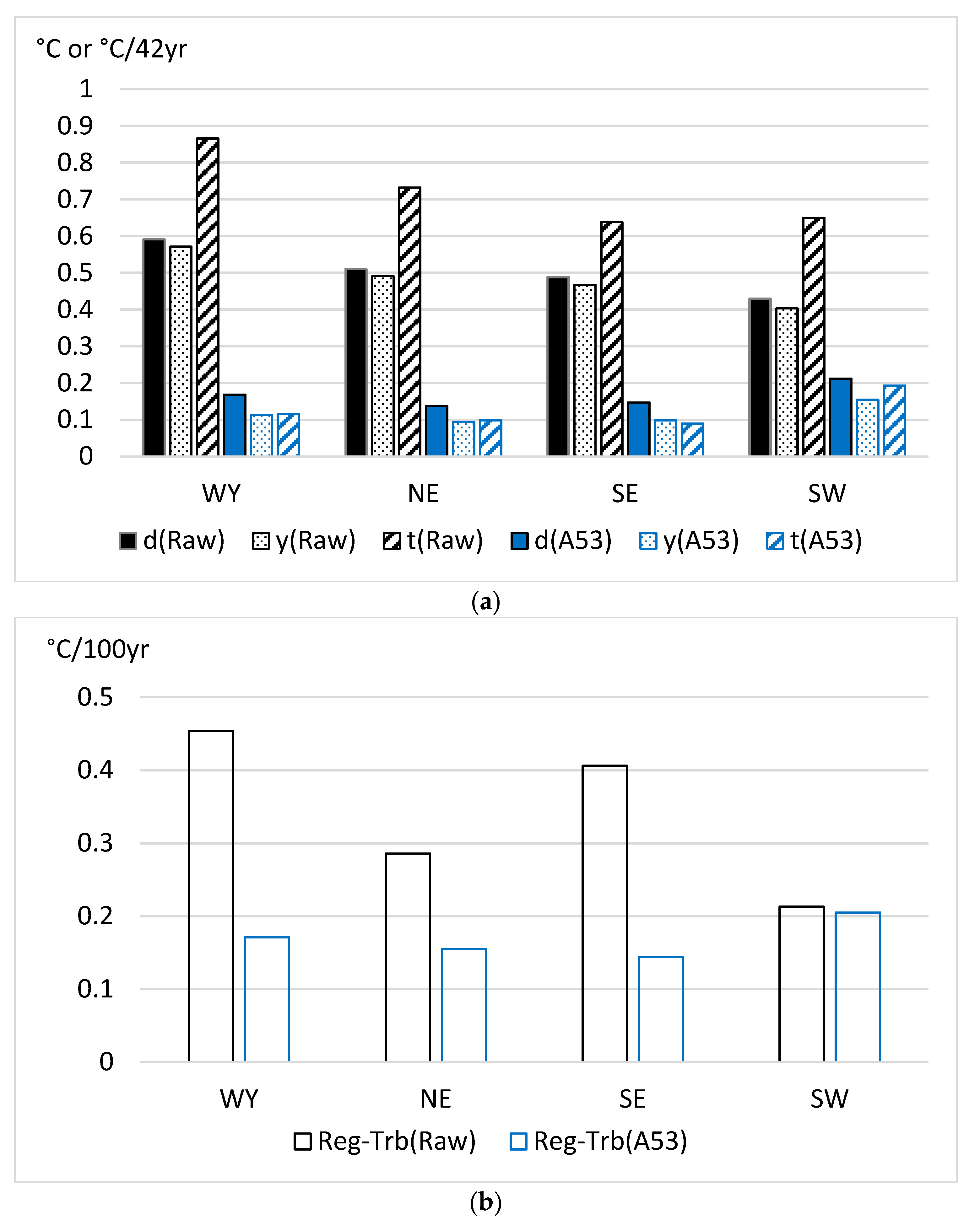
Figure 1 shows the inhomogeneity bias reduction using the A53 method in the 13 sections of the original, dense K2016 dataset.
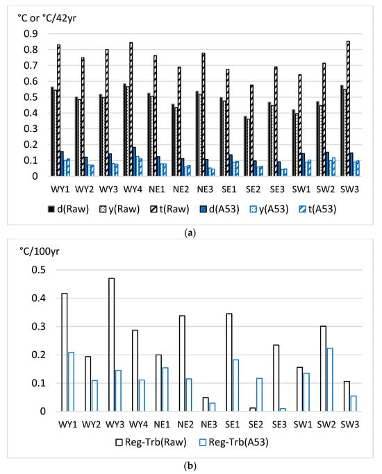
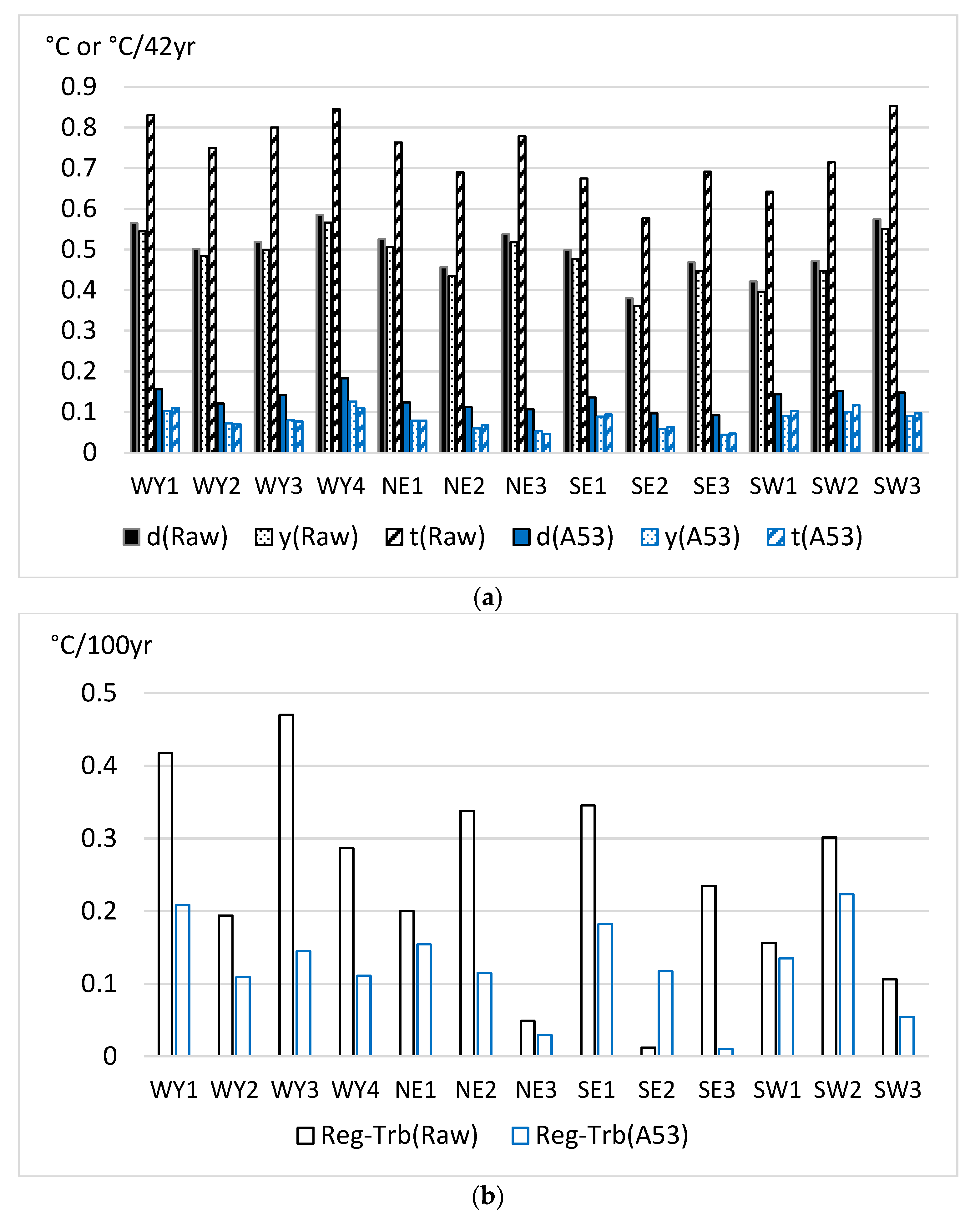
Figure 1.
Raw data errors and residual errors after homogenization with method A53 for the 13 sections of the original (dense) K2016 dataset [13]. Upper panel (a) d—RMSE of daily values; y—RMSE of annual means; t—mean absolute trend bias (Trb) for station series. Lower panel (b) Reg-Trb—regional mean absolute trend bias. Note: trend bias for station series is shown in °C per length of time series (42 years) unit for better visualization.
Figure 1a shows that high ratios of the raw data errors are removed in all error types of daily RMSE, annual RMSE and trend bias for the individual time series. The highest error reduction is achieved for the Trb of the individual series. By contrast, the error reduction in the regional mean trend bias (Figure 1b) is much smaller, but note that the regional mean trend biases of the raw data are generally small, particularly if the shortness of the time series (42 years) is also considered. When the found efficiencies according to error types are ranked from the highest to the lowest, the order is Trb for individual time series, annual RMSE, daily RMSE and Trb for the regional mean series. This rank order is typical for homogenization results, and it was found in several other studies [16,21] with the only difference that the monthly RMSE is tested instead of the daily RMSE when the test data have a monthly resolution. In the present test results, the error reductions in RMSE and Trb for individual time series are higher than in many other tests, mainly for the high station density, high spatial correlations and generally high SNR in the K2016 dataset.
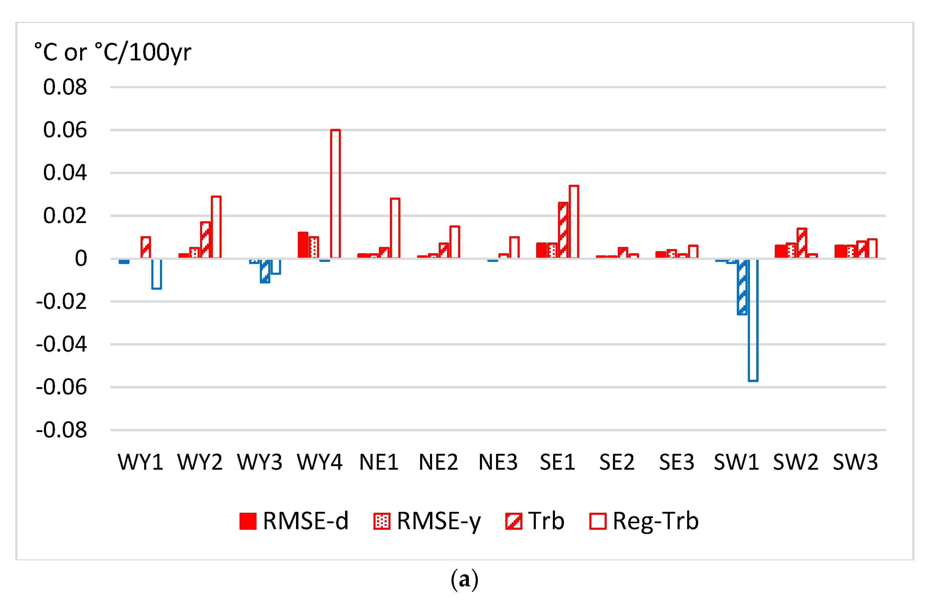
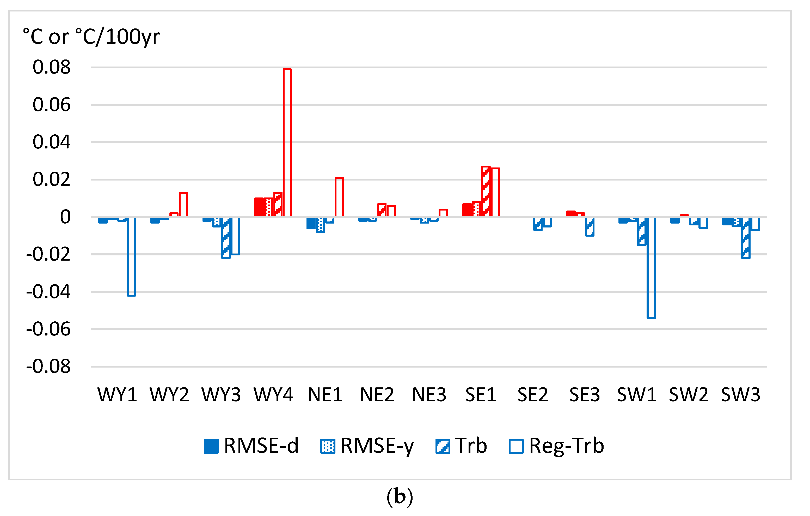
In Figure 2 the residual homogenization errors are compared between different ACMANT versions. Figure 2a compares the results of A52 and ACMANTv4, while Figure 2b shows the same comparison for A53 and ACMANTv4.
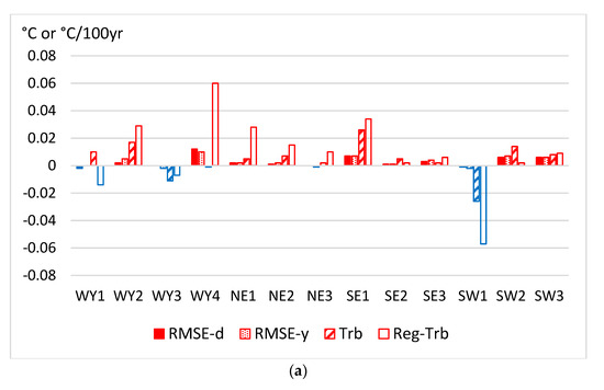

Figure 2.
Differences between homogenization errors when comparing ACMANTv5 versions to ACMANTv4 using the dense dataset. Upper panel (a) comparison of A52 and ACMANTv4; lower panel (b) comparison of A53 and ACMANTv4. Trb—mean absolute trend bias for station series; Reg-Trb—regional mean absolute trend bias.
Increasing (decreasing) errors relative to ACMANTv4 results are shown with red (blue) color. Figure 2a shows that although the absolute values of differences are small, the dominance of positive sign changes indicates that the errors with A52 are mostly larger than with ACMANTv4. The typical magnitude of the difference is lower than 0.02 °C RMSE or 0.02 °C/100 yr Trb. In the trend bias results, and particularly in the regional mean trend bias results, the differences between A52 and ACMANTv4 results are sometimes larger. Note, however, that this difference in the magnitude of differences is likely for the relatively large sampling errors of regional trend bias values (there are only 13 regions). The presence of sampling errors in the results explains that a large error decrease from ACMANTv4 to A52 also occurred (in region SW1), which, however, does not change much in the generally unfavorably picture regarding the A52 results.
Figure 2b shows that the A53 results tend to be more accurate than the ACMANTv4 results, although the magnitudes of the differences are very small. The regional trend bias results are exceptions. No decreasing tendency can be found for them, i.e., in six regions the A53 results are the most accurate, in further six regions the ACMANTv4 results are the most accurate, while in one region the regional trend bias is exactly the same with any of the two examined methods.
6.2. Results for the Moderately Dense Dataset
Figure 3 shows the residual errors of homogenization with A53 in comparison with the raw data errors.
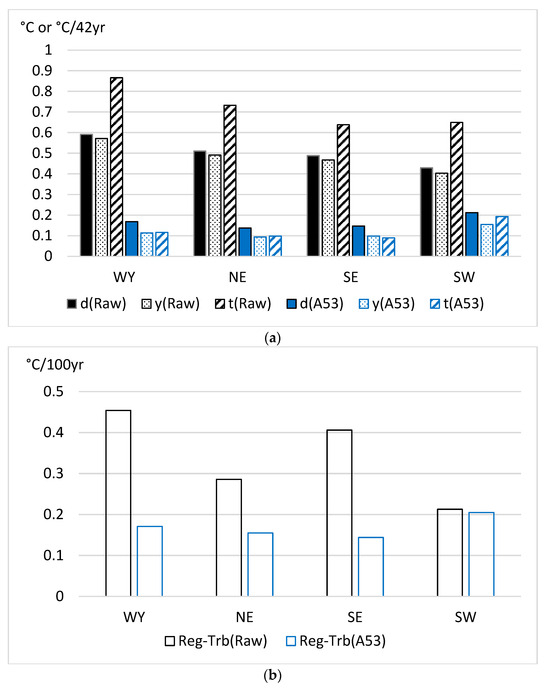
Figure 3.
Mean raw data errors and mean residual errors after homogenization with method A53 for the four main sections of the moderately dense dataset. Upper panel (a) d—RMSE of daily values; y—RMSE of annual means; t—mean absolute trend bias for station series. Lower panel (b) Reg-Trb—regional mean absolute trend bias. Note: trend bias for station series is shown in °C per length of time series (42 years) unit for better visualization.
The results of Figure 3 show that the reduction in station density relative to that of the original dataset has little effect on the homogenization accuracy, except for in the SW region where the error increase relative to the errors of the dense dataset is notable.
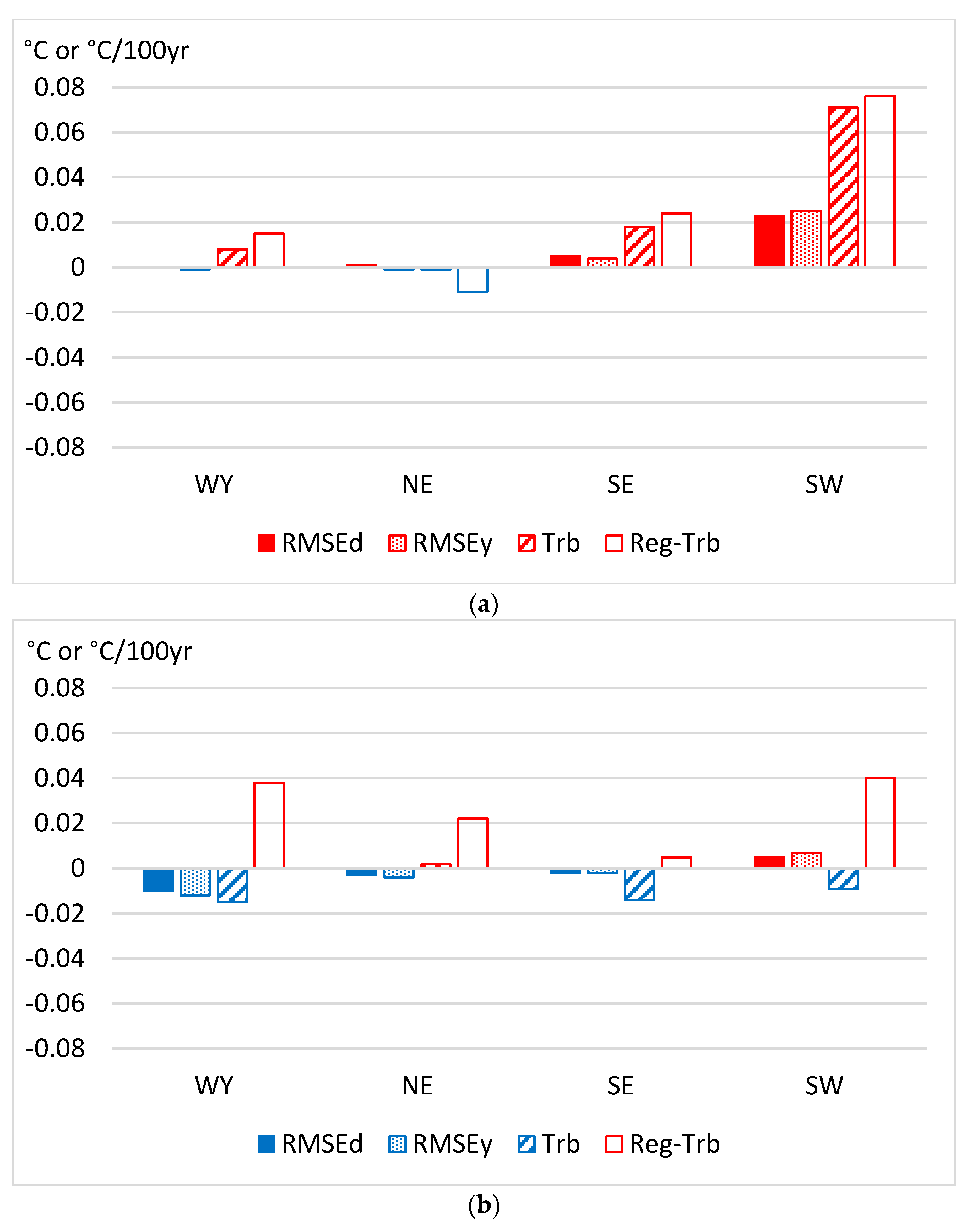
In Figure 4 the residual homogenization errors of A52 and A53 are compared to those of the ACMANTv4 results in the same way as they were compared in Figure 2 for the dense test dataset.

Figure 4.
Differences between homogenization errors when comparing ACMANTv5 versions to ACMANTv4 using the moderately dense test dataset. Each piece of the results is an average for 10 subsections of the test dataset. Upper panel (a) comparison of A52 and ACMANTv4; lower panel (b) comparison of A53 and ACMANTv4. Trb—mean absolute trend bias for station series, Reg-Trb—regional mean absolute trend bias.
In comparing the A52-ACMANTv4 differences between the results of Figure 4a and those of Figure 2a, one can find both similarities and notable differences. An important similarity between Figure 4a and Figure 2a is the dominance of red color indicating generally poorer results for A52 than for ACMANTv4. However, an important difference is that the regional differences are generally larger in Figure 4a. Here, the difference between A52 and ACMANTv4 results is practically zero for the WY and NE regions, the differences are higher for the SE region and the highest for the SW region. These results indicate that false breaks for the complexity of spatial-temporal climatic structures (see Table 1 in Section 3.1) may have a greater effect on the homogenization results when the station density is moderated, and they affect the accuracy of A52 more than the accuracy of ACMANTv4.
In Figure 4b the regional differences are smaller than in Figure 4a, and most pieces of the A53 results indicate small improvement in comparison with the ACMANTv4 results. However, the regional trends are exceptions, for them the ACMANTv4 results are better. When the frequency of false breaks is low (Table 1), the reduction in network size between A52 and A53 caused an improvement in the RMSE errors but worsening in the regional trend estimations. These results are concordant with the results of an earlier study where the network size effect on the homogenization accuracy was examined [62] with ACMANTv3 and with large surrogate datasets based on a WY section of the K2016 dataset.
6.3. Z-Index of Accuracy Improvement
Z-index values are examined for the averages of homogenization errors in the 13 (40) sections of the dense (moderately dense) datasets. Table 3 presents the results.
Table 3.
Z-index (percentage) of the change in homogenization errors when comparing versions A52 and A53 of ACMANTv5 to ACMANTv4. Mean results for entire datasets. RMSE-d—RMSE of daily values; RMSE-y—RMSE of annual values; Trb—mean absolute trend bias for station series; and Reg-Trb—regional mean absolute trend bias for dataset sections.
The reduction in network size between the A52 and A53 methods results in a small, but systematic accuracy improvement in the RMSE and station-specific trend estimations. However, the results are less clear for the regional trend bias: in dense datasets the network size reduction improved the results, while in the moderately dense dataset the regional trend estimations are almost the same with A52 and A53, and they are both poorer than with ACMANTv4. The advantage of ACMANTv4 in the regional trend estimations seems to be notable in the Z-index results, but note that the absolute differences are very small, as shown in Section 6.1 and Section 6.2.
7. Discussion
The results show generally small differences between the accuracies of the tested method versions, therefore one question is whether such small differences merit attention. I think the correct answer is yes, for two main reasons:
- (i)
- Homogenization methods are applied for several climate variables and for data observed under varied geographical conditions and using varied observation practices. Therefore, the differences found between homogenization efficiencies might be related to larger and more important absolute differences in climate characteristics than those for the K2016 dataset.
- (ii)
- Small differences in the mean errors often indicate more significant differences in the risk of committing large homogenization errors. This was demonstrated with the MULTITEST results [16,29].
The results from the K2016 dataset do not show any advantage of the pre-homogenization with combined time series comparisons, and the regional mean trend errors were found to be larger with the ACMANTv5 versions than with ACMANTv4. The likely reason for the disappointing weak results with methods including the combined time series comparison is that regional mean trend biases are generally very small in the K2016 dataset, which, however, is not rare in real observational datasets. As the accuracy of regional mean trends is a particularly important issue in climate science [29,46,47], the found problems need further research. The differences in the two experimental versions of ACMANTv5 relative to ACMANTv5.1 have the greatest influence on the homogenization of large datasets and the automatic networking procedure, while their effect is minor on previously defined small networks like most segments of the MULTITEST dataset. Therefore, the results of a comparison between ACMANTv4 accuracy and ACMANTv5 accuracy in an earlier study [18] in which the MULTITEST dataset and ACMANTv5.1 were used are considered to be usable for the joint analysis with the results of this study. Given that ACMANTv5 performed better than ACMANTv4 in most sections of the MULTITEST dataset, some slight advantage of the combined time series comparison can be concluded by the joint evaluation. The use of reduced network size in A53 is found to be more favorable than the former parameterization of automatic networking included in A52 and in previous ACMANT versions. Note, however, that these evaluations do not free from the subjectively judged importance dedicated to individual pieces of the results, and later tests might lead to other conclusions. One key issue of the further progress in relative homogenization is to learn more about the frequency and magnitude of low frequency changes in climatic gradients between time series with seemingly sufficient spatial correlations. To find reliable answers to these questions, the development of homogeneous surrogate datasets should be continued using the method started with the creation of the K2016 dataset, but further climatic zones and further climatic variables should be included.
A peculiarity of the automatic networking with A53 is that the old parameterization is used in only one break detection step of the procedure, i.e., in the second step of the combined time series comparison. There, the use of larger networks is advantageous since only relatively large breaks are searched by using a stricter significance threshold than in the other break detection steps [12]. Stricter significance thresholds could also be used in the pairwise detection step of the combined comparisons but experiments with them (not shown) did not yield better results than when the original parameterization of ACMANTv5 [18] is used.
The A53 version of ACMANT was selected as the base for further methodological developments, but later research results might modify this preference in three different ways: (i) it is possible that a more effective method of combining pairwise comparisons and the use of composite reference series will be found; (ii) future tests might indicate the superiority of the ensemble pre-homogenization method of ACMANTv4; or (iii) the method of pre-homogenization will depend on some parameters and/or previously calculated statistics for the input data in a possible future version of ACMANT. Nevertheless, regarding the available homogenization methods, both of the ACMANTv5 and ACMANTv4 methods are recommended since the inclusion of the ANOVA correction model, bivariate homogenization (when applicable) and ensemble homogenization provide the superior performance of the analyzed ACMANT versions in comparison with many other homogenization methods.
8. Conclusions
Some versions of the ACMANT homogenization method were tested with the original dense version and with a derived moderately dense version of the synthetic daily temperature dataset developed for four U.S. regions (K2016 dataset) [13]. Two experimental versions of ACMANTv5, referred to as A52 and A53, were used, and the changes in homogenization accuracy relative to the ACMANTv4 accuracy were analyzed. The main conclusions are summarized as follows:
- The found differences between ACMANTv5 accuracy and ACMANTv4 accuracy are generally small, and ACMANTv5 often gave slightly worse results than ACMANTv4.
- A reduction in network sizes reduced the RMSE and station specific trend errors of ACMANTv5, while it did not change the regional mean trend biases significantly.
- Regional mean trend biases are particularly sensitive both to the simulated climate properties of the test dataset and to the fine details of the applied homogenization method. Therefore, further improvements in the creation and use of more high-quality homogenous test datasets are needed.
- The joint analysis of the results of this study and an earlier study indicates that the inclusion of combined time series comparison in ACMANT is likely favorable.
The results of this study confirm that both of the ACMANTv4 and ACMANTv5 methods are efficient and recommended tools for the preparation of observed climatic data for climate change and climate variability studies.
Funding
This research received no external funding.
Data Availability Statement
Not applicable.
Conflicts of Interest
The author declares no conflict of interest.
References
- Moberg, A.; Alexandersson, H. Homogenization of Swedish temperature data. Part II: Homogenized gridded air temperature compared with a subset of global gridded air temperature since 1861. Int. J. Climatol. 1997, 17, 35–54. [Google Scholar] [CrossRef]
- Auer, I.; Böhm, R.; Jurkovic, A.; Orlik, A.; Potzmann, R.; Schöner, W.; Ungersböck, M.; Brunetti, M.; Nanni, T.; Maugeri, M.; et al. A new instrumental precipitation dataset for the Greater Alpine Region for the period 1800–2002. Int. J. Climatol. 2005, 25, 139–166. [Google Scholar] [CrossRef]
- Begert, M.; Schlegel, T.; Kirchhofer, W. Homogeneous temperature and precipitation series of Switzerland from 1864 to 2000. Int. J. Climatol. 2005, 25, 65–80. [Google Scholar] [CrossRef]
- Menne, M.J.; Williams, C.N.; Vose, R.S. The U.S. Historical Climatology Network Monthly Temperature Data, Version 2. Bull. Am. Meteor. Soc. 2009, 90, 993–1008. [Google Scholar] [CrossRef]
- Haimberger, L.; Tavolato, C.; Sperka, S. Homogenization of the global radiosonde temperature dataset through combined comparison with reanalysis background series and neighboring stations. J. Clim. 2012, 25, 8108–8131. [Google Scholar] [CrossRef]
- Nguyen, K.N.; Quarello, A.; Bock, O.; Lebarbier, E. Sensitivity of change-point detection and trend estimates to GNSS IWV time series properties. Atmosphere 2021, 12, 1102. [Google Scholar] [CrossRef]
- Szentimrey, T. Multiple Analysis of Series for Homogenization (MASH). In Second Seminar for Homogenization of Surface Climatological Data; Szalai, S., Szentimrey, T., Szinell, C., Eds.; WMO WCDMP-41; WMO: Geneva, Switzerland, 1999; pp. 27–46. [Google Scholar]
- Caussinus, H.; Mestre, O. Detection and correction of artificial shifts in climate series. J. R. Stat. Soc. Ser. C Appl. Stat. 2004, 53, 405–425. [Google Scholar] [CrossRef]
- Menne, M.J.; Williams, C.N., Jr. Homogenization of temperature series via pairwise comparisons. J. Clim. 2009, 22, 1700–1717. [Google Scholar] [CrossRef]
- Mestre, O.; Domonkos, P.; Picard, F.; Auer, I.; Robin, S.; Lebarbier, E.; Böhm, R.; Aguilar, E.; Guijarro, J.; Vertacnik, G.; et al. HOMER: Homogenization software in R—Methods and applications. Időjárás 2013, 117, 47–67. [Google Scholar]
- Guijarro, J.A. Homogenization of Climatic Series with Climatol; 2018. Available online: http://www.climatol.eu/homog_climatol-en.pdf (accessed on 25 September 2023).
- Domonkos, P. ACMANTv4: Scientific Content and Operation of the Software; 2020, 71p. Available online: https://github.com/dpeterfree/ACMANT/blob/ACMANTv4.4/ACMANTv4_description.pdf (accessed on 25 September 2023).
- Killick, R.E. Benchmarking the Performance of Homogenisation Algorithms on Daily Temperature Data. Ph.D. Thesis, University of Exeter, Exeter, UK, 2016. Available online: https://ore.exeter.ac.uk/repository/handle/10871/23095 (accessed on 5 November 2023).
- Chimani, B.; Venema, V.; Lexer, A.; Andre, K.; Auer, I.; Nemec, J. Inter-comparison of methods to homogenize daily relative humidity. Int. J. Climatol. 2018, 38, 3106–3122. [Google Scholar] [CrossRef]
- Guijarro, J.A. Recommended Homogenization Techniques Based on Benchmarking Results. WP-3 Report of INDECIS Project. 2019. Available online: http://www.indecis.eu/docs/Deliverables/Deliverable_3.2.b.pdf (accessed on 25 September 2023).
- Domonkos, P.; Guijarro, J.A.; Venema, V.; Brunet, M.; Sigró, J. Efficiency of time series homogenization: Method comparison with 12 monthly temperature test datasets. J. Clim. 2021, 34, 2877–2891. [Google Scholar] [CrossRef]
- Guijarro, J.A.; López, J.A.; Aguilar, E.; Domonkos, P.; Venema, V.K.C.; Sigró, J.; Brunet, M. Homogenization of monthly series of temperature and precipitation: Benchmarking results of the MULTITEST project. Int. J. Climatol. 2023, 43, 3994–4012. [Google Scholar] [CrossRef]
- Domonkos, P. Combination of using pairwise comparisons and composite reference series: A new approach in the homogenization of climatic time series with ACMANT. Atmosphere 2021, 12, 1134. [Google Scholar] [CrossRef]
- Joelsson, L.M.T.; Sturm, C.; Södling, J.; Engström, E.; Kjellström, E. Automation and evaluation of the interactive homogenization tool HOMER. Int. J. Climatol. 2022, 42, 2861–2880. [Google Scholar] [CrossRef]
- Szentimrey, T. Overview of mathematical background of homogenization, summary of method MASH and comments on benchmark validation. Int. J. Climatol. 2023. early view. [Google Scholar] [CrossRef]
- Venema, V.; Mestre, O.; Aguilar, E.; Auer, I.; Guijarro, J.A.; Domonkos, P.; Vertacnik, G.; Szentimrey, T.; Štěpánek, P.; Zahradníček, P.; et al. Benchmarking monthly homogenization algorithms. Clim. Past 2012, 8, 89–115. [Google Scholar] [CrossRef]
- Lindau, R.; Venema, V.K.C. The uncertainty of break positions detected by homogenization algorithms in climate records. Int. J. Climatol. 2016, 36, 576–589. [Google Scholar] [CrossRef]
- Lindau, R.; Venema, V.K.C. The joint influence of break and noise variance on the break detection capability in time series homogenization. Adv. Stat. Clim. Meteorol. Oceanogr. 2018, 4, 1–18. [Google Scholar] [CrossRef]
- Peterson, T.C.; Easterling, D.R. Creation of homogeneous composite climatological reference series. Int. J. Climatol. 1994, 14, 671–679. [Google Scholar] [CrossRef]
- Szentimrey, T. Methodological questions of series comparison. In Sixth Seminar for Homogenization and Quality Control in Climatological Databases; Lakatos, M., Szentimrey, T., Bihari, Z., Szalai, S., Eds.; WMO WCDMP-76; WMO: Geneva, Switzerland, 2010; pp. 1–7. [Google Scholar]
- Craddock, J.M. Methods of comparing annual rainfall records for climatic purposes. Weather 1979, 34, 332–346. [Google Scholar] [CrossRef]
- Kuglitsch, F.G.; Toreti, A.; Xoplaki, E.; Della-Marta, P.M.; Luterbacher, J.; Wanner, H. Homogenization of daily maximum temperature series in the Mediterranean. J. Geophys. Res. 2009, 114, D15108. [Google Scholar] [CrossRef]
- Trewin, B. A daily homogenized temperature data set for Australia. Int. J. Climatol. 2013, 33, 1510–1529. [Google Scholar] [CrossRef]
- Domonkos, P.; Tóth, R.; Nyitrai, L. Climate Observations: Data Quality Control and Time Series Homogenization; Elsevier: Amsterdam, The Netherlands, 2022; 302p. [Google Scholar]
- Rustemeier, E.; Kapala, A.; Meyer-Christoffer, A.; Finger, P.; Schneider, U.; Venema, V.; Ziese, M.; Simmer, C.; Becker, A. AHOPS Europe—A gridded precipitation data set from European homogenized time series. In Proceedings of the Ninth Seminar for Homogenization and Quality Control in Climatological Databases; Szentimrey, T., Lakatos, M., Hoffmann, L., Eds.; WMO WCDMP-85; WMO: Geneva, Switzerland, 2017; pp. 88–101. [Google Scholar]
- Domonkos, P. Efficiency evaluation for detecting inhomogeneities by objective homogenisation methods. Theor. Appl. Climatol. 2011, 105, 455–467. [Google Scholar] [CrossRef]
- Easterling, D.R.; Peterson, T.C. A new method for detecting undocumented discontinuities in climatological time series. Int. J. Climatol. 1995, 15, 369–377. [Google Scholar] [CrossRef]
- Perreault, L.; Haché, M.; Slivitzky, M.; Bobée, B. Detection of changes in precipitation and runoff over eastern Canada and U.S. using a Bayesian approach. Stoch. Environ. Res. Risk Assess. 1999, 13, 201–216. [Google Scholar] [CrossRef]
- Wang, X.L.; Wen, Q.H.; Wu, Y. Penalized maximal t test for detecting undocumented mean change in climate data series. J. Appl. Meteor. Climatol. 2007, 46, 916–931. [Google Scholar] [CrossRef]
- Alexandersson, H. A homogeneity test applied to precipitationdata. J. Climatol. 1986, 6, 661–675. [Google Scholar] [CrossRef]
- Picard, F.; Lebarbier, E.; Hoebeke, M.; Rigaill, G.; Thiam, B.; Robin, S. Joint segmentation, calling, and normalization of multiple CGH profiles. Biostatistics 2011, 12, 413–428. [Google Scholar] [CrossRef]
- Mamara, A.; Argiriou, A.; Anadranistakis, E. Detection and correction of inhomogeneities in Greek climate temperature series. Int. J. Climatol. 2014, 34, 3024–3043. [Google Scholar] [CrossRef]
- Gofa, F.; Mamara, A.; Anadranistakis, M.; Flocas, H. Developing gridded climate data sets of precipitation for Greece based on homogenized time series. Climate 2019, 7, 68. [Google Scholar] [CrossRef]
- Joelsson, L.M.T.; Engström, E.; Kjellström, E. Homogenization of Swedish mean monthly temperature series 1860–2021. Int. J. Climatol. 2023, 43, 1079–1093. [Google Scholar] [CrossRef]
- Skrynyk, O.; Aguilar, E.; Guijarro, J.; Randriamarolaza, L.Y.A.; Bubin, S. Uncertainty evaluation of Climatol’s adjustment algorithm applied to daily air temperature time series. Int. J. Climatol. 2021, 41 (Suppl. 1), E2395–E2419. [Google Scholar] [CrossRef]
- Kessabi, R.; Hanchane, M.; Guijarro, J.A.; Krakauer, N.Y.; Addou, R.; Sadiki, A.; Belmahi, M. Homogenization and trends analysis of monthly precipitation series in the Fez-Meknes region, Morocco. Climate 2022, 10, 64. [Google Scholar] [CrossRef]
- Pita-Díaz, O.; Ortega-Gaucin, D. Analysis of anomalies and trends of climate change indices in Zacatecas, Mexico. Climate 2020, 8, 55. [Google Scholar] [CrossRef]
- Coll, J.; Domonkos, P.; Guijarro, J.; Curley, M.; Rustemeier, E.; Aguilar, E.; Walsh, S.; Sweeney, J. Application of homogenization methods for Ireland’s monthly precipitation records: Comparison of break detection results. Int. J. Climatol. 2020, 40, 6169–6188. [Google Scholar] [CrossRef]
- Lindau, R.; Venema, V. On the reduction of trend errors by the ANOVA joint correction scheme used in homogenization of climate station records. Int. J. Climatol. 2018, 38, 5255–5271. [Google Scholar] [CrossRef]
- Prohom, M.; Domonkos, P.; Cunillera, J.; Barrera-Escoda, A.; Busto, M.; Herrero-Anaya, M.; Aparicio, A.; Reynés, J. CADTEP: A new daily quality-controlled and homogenized climate database for Catalonia (1950–2021). Int. J. Climatol. 2023, 43, 4771–4789. [Google Scholar] [CrossRef]
- Williams, C.N.; Menne, M.J.; Thorne, P. Benchmarking the performance of pairwise homogenization of surface temperatures in the United States. J. Geophys. Res. 2012, 117, D05116. [Google Scholar] [CrossRef]
- Menne, M.J.; Williams, C.N.; Gleason, B.E.; Rennie, J.J.; Lawrimore, J.H. The Global Historical Climatology Network monthly temperature dataset, version 4. J. Clim. 2018, 31, 9835–9854. [Google Scholar] [CrossRef]
- Thorne, P.W.; Menne, M.J.; Williams, C.N.; Rennie, J.J.; Lawrimore, J.H.; Vose, R.S.; Peterson, T.C.; Durre, I.; Davy, R.; Esau, I.; et al. Reassessing changes in diurnal temperature range: A new data set and characterization of data biases. J. Geophys. Res. Atmos. 2016, 121, 5115–5137. [Google Scholar] [CrossRef]
- Laapas, M.; Venäläinen, A. Homogenization and trend analysis of monthly mean and maximum wind speed time series in Finland, 1959–2015. Int. J. Climatol. 2017, 37, 4803–4813. [Google Scholar] [CrossRef]
- O’Neill, P.; Connolly, R.; Connolly, M.; Soon, W.; Chimani, B.; Crok, M.; de Vos, R.; Harde, H.; Kajaba, P.; Nojarov, P.; et al. Evaluation of the homogenization adjustments applied to European temperature records in the Global Historical Climatology Network Dataset. Atmosphere 2022, 13, 285. [Google Scholar] [CrossRef]
- Vincent, L.A.; Wang, X.L.; Milewska, E.J.; Wan, H.; Yang, F.; Swail, V. A second generation of homogenized Canadian monthly surface air temperature for climate trend analysis. J. Geophys. Res. 2012, 117, D18110. [Google Scholar] [CrossRef]
- Kuglitsch, F.G.; Auchmann, R.; Bleisch, R.; Brönnimann, S.; Martius, O.; Stewart, M. Break detection of annual Swiss temperature series. J. Geophys. Res. 2012, 117, D13105. [Google Scholar] [CrossRef]
- Domonkos, P. Automatic homogenization of time series: How to use metadata? Atmosphere 2022, 13, 1379. [Google Scholar] [CrossRef]
- Prohom, M.; Barriendos, M.; Sanchez-Lorenzo, A. Reconstruction and homogenization of the longest instrumental precipitation series in the Iberian Peninsula (Barcelona, 1786–2014). Int. J. Climatol. 2016, 36, 3072–3087. [Google Scholar] [CrossRef]
- Camuffo, D.; della Valle, A.; Becherini, F. Instrumental and observational problems of the earliest temperature records in Italy: A methodology for data recovery and correction. Climate 2023, 11, 178. [Google Scholar] [CrossRef]
- Fioravanti, G.; Piervitali, E.; Desiato, F. A new homogenized daily data set for temperature variability assessment in Italy. Int. J. Climatol. 2019, 39, 5635–5654. [Google Scholar] [CrossRef]
- Yosef, Y.; Aguilar, E.; Alpert, P. Changes in extreme temperature and precipitation indices: Using an innovative daily homogenized database in Israel. Int. J. Climatol. 2019, 39, 5022–5045. [Google Scholar] [CrossRef]
- Adeyeri, O.E.; Laux, P.; Ishola, K.A.; Zhou, W.; Balogun, I.A.; Adeyewa, Z.D.; Kunstmann, H. Homogenising meteorological variables: Impact on trends and associated climate indices. J. Hydrol. 2022, 607, 127585. [Google Scholar] [CrossRef]
- Molina-Carpio, J.; Rivera, I.A.; Espinoza-Romero, D.; Cerón, W.L.; Espinoza, J.-C.; Ronchail, J. Regionalization of rainfall in the upper Madeira basin based on interannual and decadal variability: A multi-seasonal approach. Int. J. Climatol 2023. early view. [Google Scholar] [CrossRef]
- Compo, G.P.; Whitaker, J.S.; Sardeshmukh, P.D.; Matsui, N.; Allan, R.J.; Yin, X.; Gleason, B.E., Jr.; Vose, R.S.; Rutledge, G.; Bessemoulin, P.; et al. The twentieth century reanalysis project. Q. J. R. Meteorol. Soc. 2011, 137, 1–28. [Google Scholar] [CrossRef]
- Domonkos, P. Manual of ACMANTv5. 2021. Available online: https://github.com/dpeterfree/ACMANT/tree/ACMANTv5_documents (accessed on 25 September 2023).
- Domonkos, P.; Coll, J. Time series homogenisation of large observational datasets: The impact of the number of partner series on the efficiency. Clim. Res. 2017, 74, 31–42. [Google Scholar] [CrossRef]
Disclaimer/Publisher’s Note: The statements, opinions and data contained in all publications are solely those of the individual author(s) and contributor(s) and not of MDPI and/or the editor(s). MDPI and/or the editor(s) disclaim responsibility for any injury to people or property resulting from any ideas, methods, instructions or products referred to in the content. |
© 2023 by the author. Licensee MDPI, Basel, Switzerland. This article is an open access article distributed under the terms and conditions of the Creative Commons Attribution (CC BY) license (https://creativecommons.org/licenses/by/4.0/).