Abstract
Tropical cyclones (TCs) are one of the most destructive natural hazards to impact on Australia’s population, infrastructure, and the environment. To examine potential TC impacts, it is important to understand which assets are exposed to the hazard and of these, which are vulnerable to damage. The aim of this study is to improve TC risk assessments through developing an exposure–vulnerability index, utilising a case study for the six Local Government Areas (LGAs) impacted by the landfall of TC Debbie in 2017: Burdekin Shire, Charters Towers Region, Isaac Region, Mackay Region, City of Townsville, and Whitsunday Region. This study utilised a natural hazard risk assessment methodology, linking exposure and vulnerability indicators related to social factors, infrastructure, and the environment. The two LGAs with the most extreme exposure–vulnerability values were the coastal regions of Mackay Region and the City of Townsville. This is consistent with urbanisation and city development trends, with these LGAs having more people (social) and infrastructure exposed, while the environmental domain was more exposed and vulnerable to TC impacts in rural LGAs. Therefore, further resilience protocols and mitigation strategies are required, particularly for Mackay Region and the City of Townsville, to reduce the damage and ultimate loss of lives and livelihoods from TC impacts. This study serves as a framework for developing a TC risk index based on hazard, exposure, and vulnerability indices, and insight into the improved mitigation strategies for communities to implement in order to build resilience to the impacts of future TCs.
1. Introduction
Natural hazards are environmental phenomena that have the potential to produce negative impacts on society and the natural environment, resulting in the loss of life, injury, damage, or degradation [1]. Described as one of the most pertinent and devastating natural hazards facing Australia [2], tropical cyclones (TCs) are severe, multi-hazard weather phenomena, generating destructive winds, heavy rainfall, and coastal storm surges, which all contribute to destructive impacts on population, infrastructure, and the environment [3].
The impacts of TCs in the Pacific region exhibit a wide range of effects that are both diverse and disastrous [4]. Whether it be for small island developing states with fragile economies or for developed Pacific island countries like Australia, impacts manifest differently and are modulated by the socio-environmental conditions of the region they make landfall on [5,6]. Although TCs are most harmful to small islands and fragile economies, they have made a large imprint in Australia [7]. Long-term records demonstrate that on average eleven TCs occur in the Australian region each year [8]. The total cost of TCs in Australia has amassed to AUD 23 billion since 1967 [9] and resulted in the loss of an estimated 206 lives from 1970–2017 within Australia directly from TC impacts [10].
Climate change increases the range of impacts from natural hazards, including their socio-ecological interactions, scale, location, timing, and frequency [11]. The projected increasing intensity of TCs due to anthropogenic climate change will have profound implications for the sustainability of societies, ecosystems, and biodiversity, and so must be addressed systematically and comprehensively [2,12,13,14].
Through TCs’ potential devastation in Australia, there is a bolstered ambition within the scientific landscape to develop mechanisms to assess natural hazard risks [13,15]. Correctly defining natural hazard risk terminology is critical due to its contribution to informing stakeholders and decision makers on TC risk reduction procedures. The definitions of risk terminology vary amongst the literature. In this study, the definitions from the Intergovernmental Panel on Climate Change (IPCC) have been adopted [13]. Natural hazard risk is defined by the IPCC as “the possibility for adverse implications for human or ecological systems from natural hazards” [13]. To combat the rising concern over natural hazard risks, there has been an emphasis on the application of a natural hazard risk assessment (NHRA) to ultimately inform decision makers and critical stakeholders when developing mitigation and adaptation strategies for exposed and vulnerable communities [16]. Thus, decision makers and stakeholders can identify at-risk regions in advance and develop appropriate measures to reduce mortality, damages, and economic losses from potential TC impacts in the future [17].
With the anthropogenic influence of climate change, an NHRA enables an effective approach to generate evaluation techniques for local study areas [13]. This allows for long-term socio-economic adaptation and response mechanisms, improving the possible disaster resilience of a community in both the short-term and long-term [13,18].
Additionally, the escalating chance of societal, infrastructural, and environmental impacts from TCs demands further investigation into early warning systems and mitigation strategies, including TC risk assessments [19]. Risk assessments are paramount due to the multi-hazard implications associated with TCs within Australia’s coastal regions, requiring further attention and risk management [20].
Natural hazard risk is typically conceptualised as a risk triangle [21]. It explains risk as the product of three components presented in Equation (1):
where hazard is defined as “the potential occurrence of a natural hazard event that may cause loss of life, injury, or other health impacts, as well as damage and loss to property infrastructure, livelihoods, and service provision” [13]. Exposure is defined as “the presence of people; livelihoods; species or ecosystems; environmental functions, services and resources; infrastructure; or economic, social or cultural assets in place and settings that could be adversely affected [by a natural hazard]” [13]. Vulnerability is defined as “the propensity or predisposition to be adversely affected [by a natural hazard] and encompasses a variety of concepts and elements, including sensitivity or susceptibility to harm and lack of capacity to cope and adapt” [13].
Risk = Hazard × Exposure × Vulnerability
Although NHRA can be conducted using a variety of methods and environments, it is found to be most effective and useful when tailored to a specific spatial context, including resolutions of Local Government Areas (LGAs) [22]. This allows research to arrive at evidence-based conclusions and recommendations for local decision makers and stakeholders in disaster risk reduction strategies [22,23,24,25].
For Australia-based TC risk, the exposed assets that are most susceptible to damage tend to be critical infrastructure including hospitals and residential housing, and environment landscapes including cropland and coral reefs [26].
To evaluate the contribution of specific characteristics of exposure and vulnerability to the risk of a natural hazard, an index can be used to quantify the impact. Multi-Criteria Decision-Making techniques, referred to as indices within this study [27], provide weighting to key criteria to posit comparative information for decision-making analyses. Several TC exposure and vulnerability indices can then be paired with TC hazard indices to calculate the overall TC risk. With indices being composed of community-focused indicators, maps can be generated and analysed to highlight the most at-risk areas.
The aim of this study is to improve TC risk assessments through developing an exposure–vulnerability index. Listed below are the research gaps of this study. First, in earlier studies, when doing a cross-comparison between exposure and vulnerability for TC risk assessments, when exposure and vulnerability indices are paired, the indicators are incongruous [28]. An example of this is seen in the TCs’ risk assessment by Do and Kuleshov [28], who links coral density and unemployment rate in the same index. Linking uncorrelated indicators ultimately reduces the value of the exposure–vulnerability index for decision makers, as they may have information on how exposed a particular asset is, but not on how vulnerable this asset is to damage. Vulnerability indicators mostly focus on socially oriented themes, including unemployment rate and socio-economic disadvantage, whilst exposure is often composed of social, physical, and environmental indicators [28,29,30,31,32,33]. However, by linking the exposure indicators with related vulnerability indicators, stakeholders have greater insight into specific resilience structures and mitigation strategies moving forward.
In this study, we link exposure and vulnerability indicators following the method of Peduzzi, et al. [34]. Each vulnerability indicator will be directly linked to the exposure indicator to ensure appropriateness in the index alignment between the three domains of social, physical, and environmental. An example of this could include pairing the exposure indicator of population density with the vulnerability indicator of unemployment rate, between which there is a known relationship [35]. Indices will be created for all of the three domains of social, infrastructure, and environment, and then for a complete exposure–vulnerability index. The suitability of linking exposure indicators with related vulnerability indicators is confirmed by the effectiveness of the risk assessment generated by Peduzzi et al. [34], who utilised this methodology, and in the work by Do and Kuleshov [28], who explain that the lack of linking between indicators is a limitation of their study. Additionally, each index of exposure and vulnerability will both have indicators for all social, infrastructure, and environment factors.
Second, Multi-Criteria Decision-Making technique studies have seldom been conducted in Australia, despite international use in recent years [36,37,38,39]. Additionally, the TC risk assessments conducted in Australia are not community-specific—being nationwide rather than examining smaller regions in depth. By analysing community-specific TC risk assessments, this study provides decision makers with insight into what community-specific assets are exposed and also vulnerable to damage, and thus increasing their ability to implement more community-focused resilience structures and mitigation strategies. In this study, a community-specific exposure–vulnerability index will be developed for the eastern coast of Australia, with the study area localised to the six surrounding LGAs where TC Debbie made landfall in 2017. All indicators will be related to the impacts and settings of these six LGAs.
Third, there has historically been an equal weighting of indicators, rather than having them weighted based on their contextual significance [28,40]. By weighing them based on their influence, this spotlights the most critical assets that are exposed and vulnerable to damage, inspiring an improved ability to implement mitigation strategies that will save the most lives and livelihoods. This study will use a weighting approach through a Principal Component Analysis (PCA), explained further in Section 2.8.
Ultimately, this study adopts an approach to TC risk assessments through linking exposure and vulnerability indicators together within the three domains of social, infrastructure, and environment, which have been weighted by impact, to generate a single index, and performing this in a specific location within the eastern coast of Australia.
2. Materials and Methods
2.1. Study Area
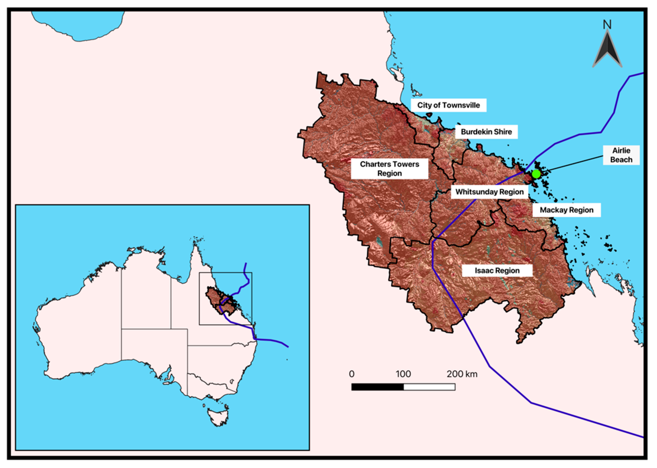
TC Debbie made landfall on the 28 March 2017 [41]. Causing AUD 3.5 billion in damage and fourteen deaths primarily through extreme riverine and coastal flooding, this event has gained a reputation as one of the most destructive TC events in Australian recorded history [41,42,43]. With TC Debbie making landfall by Airlie Beach, Queensland, and progressing southward to New South Wales, this TC event covered an extensive geographical scale. To ensure that this study is specific to the TC Debbie event, Figure 1 displays the six LGAs surrounding landfall that will be utilised as the study area, including Burdekin Shire, Charters Towers Region, Isaac Region, Mackay Region, City of Townsville, and Whitsunday Region.
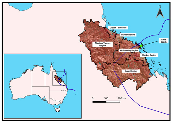
Figure 1.
Study area of six Local Government Areas surrounding TC Debbie landfall near Airlie Beach, marked by the green dot, with the blue line representing the TC Debbie track (generated using QGIS 3.30 software).
The exposure–vulnerability index developed in this study prioritises indicators that directly impact human health and livelihoods, in accordance with the exposure and vulnerability definitions adopted by the IPCC. To the best of our knowledge, this is the first exposure–vulnerability assessment to make use of this study area, which is of particular importance being a highly TC-prone region in Australia.
2.2. Selecting Tropical Cyclone Indicators
Indicators for both exposure and vulnerability were identified for the three domains of social, infrastructure, and environment. The selection of the indicators was contingent on the impacts experienced by the LGAs within the study area, as well as the data available. Table 1 provides a summary of the indicators, while a full definition of the indicators is provided in Section 2.3 and Section 2.4.

Table 1.
Exposure and vulnerability indicators utilised within the three domains of social, infrastructure, and environment.
The two domains of social and infrastructure, seen in Table 1, were evaluated because of their historical prevalence in risk assessments [3,22,29]. The third domain, environment, is less prevalent in the literature, yet, in combination with social and infrastructural factors, it provides a holistic assessment of the exposure and vulnerability within society [28].
Table 2 displays where the indicators were sourced, alongside the datasets’ resolution and year of release.

Table 2.
The datasets, sources, resolution, and year of release for each indicator within the two risk groups of exposure and vulnerability.
2.3. Exposure
2.3.1. Population Density
Population density is a common social exposure indicator for community exposure during a natural hazard including TC events [3,40,44]. This indicator can be calculated by dividing the estimated resident population by the land area, and so measures the number of people living in a designated region that could be negatively impacted by a TC event. There is a positive correlation between population density and TC exposure where an increase in population density results in greater TC exposure. Increased TC exposure leads to a larger number of people that can be affected by TC damage, causing a loss of lives and livelihoods.
2.3.2. Hospitals
Hospitals are utilised as an infrastructural exposure indicator within this study. Hospitals are used for TC risk assessments due to their important role in providing health-care services and supporting emergency response efforts. Humans are frequently injured from TC events, particularly from moving debris and in some cases infrastructural collapse, and thus need medical attention [45,46]. There is a positive correlation between hospital numbers and exposure; LGAs with more hospitals are more exposed. An extreme level of exposure for this indicator demonstrates high levels of hospitals that can be exposed to TC impacts.
The locations of private and public hospitals were downloaded as a CSV file to then be imported into QGIS with their geographical coordinates.
2.3.3. Residential Housing
To quantify the impact of a TC on the physical environment, another prominent infrastructure asset is the dwelling areas of the people within that region. In the study area, the most common dwelling area is residential housing, and so this is a pertinent indicator for infrastructural exposure. There is a positive relationship between residential housing and exposure, where an increase in residential housing increases the number of assets exposed to the potential harms of TCs. Residential housing was obtained through a Digital Cadastre dataset, providing a spatial representation of each current parcel of land within the study area. This dataset is considered a point of verity for the graphical representation of property boundaries. Obtained on 1 May 2023, this dataset is updated weekly on each Sunday from the Lands Address Location Framework database [47]. This foundational dataset contains the number, street, locality, and coordination referee(s) for property addresses in the study area.
2.3.4. Land Use Land Cover (LULC)
LULC is a common natural hazard environmental exposure indicator, also typically found in TC studies [27]. LULC posits the different land types which exist in a given area based on their use. Mapped by the Australian Land Use and Management Classification, the Queensland Government maps and assesses the land use patterns and changes across regions.
The LULC indicator was created using QGIS version 3.30.1’s Hertogenbosch software. The Land Use of Australia 2010–2011 to 2015–2016, 250 m dataset, based on the 2021 census, is a product of the Australian Collaborative Land Use and Management Program. To correlate LULC with community exposure, each LULC has been attributed with a weight classification depending on their value in the context of TC exposure, where higher values indicate more community value and hence greater TC exposure. Thematic layers of land use were compartmentalised into eight classifications, seen in Table 3. Thereafter, each classification was assigned a value for the potential impact that exposed assets in this LULC indicator can be afflicted by a TC event.

Table 3.
Reclassified LULC, with respective values and ratings, for the LULC indicator.
Whilst sometimes open to subjectivity, this reclassification and valuing system is prevalent throughout the literature and is an effective way to quantitatively categorise qualitative land use classes [27,40,48,49]. Additionally, this method has been conducted based on a comprehensive understanding and informed decisions about LULCs within this study scope. Thus, this method is suitable for such a study. There is a positive relationship between LULC and exposure; as the LULC weighted value increases, the greater the exposure of the asset to the harms of TC events.
2.4. Vulnerability
2.4.1. Index of Relative Socio-economic Disadvantage (IRSD)
The IRSD, a component of the Socio-Economic Indexes for Areas (SEIFA), is a comprehensive index created by the Australian Bureau of Statistics (ABS). This index differs from other indices in that it solely describes the factors of relative disadvantage, which effectively captures the non-TC conditions that render the community highly vulnerable. The adoption of the IRSD as a social vulnerability indicator is advantageous as the variables included are multifaceted. Described in Appendix A, the IRSD encompasses important domains of vulnerability of both economic and social dimensions.
IRSD scores are presented using quintiles (the scores are ranked and distributed into five groups, with each group representing 20% of the distribution), whereby the lowest scoring 20% of areas are assigned a quintile number of 1, up to the highest 20% of areas, which are ascribed a quintile number of 5. Low IRSD scores indicate that an area has a relatively greater socio-economic disadvantage overall. The ABS recommends that IRSD data be used when investigating broad measures of disadvantage, rather than specific measures. This is applicable to this study since a broader scope is more appropriate for assessing the data’s contribution to TC vulnerability.
The IRSD data were downloaded as an Excel dataset from the ABS website for each LGA, normalised using a logarithmic min–max approach, and then imported into the QGIS 3.30 software.
2.4.2. Vulnerable Age Groups
Defined by people aged below 15 and over 65, vulnerable age groups have seldom been used in academic literature as a social indicator to assess the vulnerability of a community to TC impact. However, through the impacts and the responses from the six LGAs identified as the study area in this study, it is clear that these categorised age groups were disproportionately affected by TC Debbie [50]. There is a positive correlation between vulnerable age groups and vulnerability, where the higher the proportion of population that fall into these two categories, the more vulnerable that population is to damage. These data were normalised on a scale of 0–1 using the logarithmic min–max method.
2.4.3. Core Assistance
Core Activity Need for Assistance (CANA) is being utilised as a social indicator for vulnerability. This indicator records the number of people with a profound or severe core activity limitation, who thus require daily assistance in one or more of the three core activities of self-care, mobility, and communication. Contributing factors, as included in the 2021 census, include long-term health conditions that have lasted for more than 6 months, a disability of over 6 months, and old age. There is a positive relationship between CANA and vulnerability, where the more people that require core assistance for daily activities, the greater the vulnerability of that population to TC impacts. These data were then normalised on a scale of 0–1 using a logarithmic min–max approach.
2.4.4. Travel to Hospital Difficulty
In a TC event, humans could be injured through collapsing buildings and moving debris, and thus require hospital services [45,46]. To measure the accessibility of health services for people in need during TC events, the social indicator for vulnerability of hospital travel difficulty can be utilised. In this study, the method for estimating travel difficulty is through the shortest distance from residential housing to hospital locations, utilising a Euclidean ‘crow flight’ approach. This approach is the shortest single, straight journey from the initial point to the final point. The residential housing dataset is found through Queensland Local Government, and in some instances, private developers. The hospital location is found through Queensland Health. The distances from residential housing to hospitals were averaged for each LGA, and normalised using a logarithmic min–max approach.
There is a positive correlation between travel to hospital difficulty and vulnerability. If the difficulty increases, indicating a longer distance, then these individuals are more vulnerable to the negative impacts from TCs.
2.4.5. Residential Housing Building Codes
The destructive winds and storm surges from TCs exert huge forces on houses with pressure pushing on the windward wall and applying high suction pressures on the roof (trying to lift the house out of the ground) [51,52]. Additionally, if a sudden opening occurs, for example, a broken window or a failed door, the windward wall pressure can suddenly enter the house and exacerbate the stress on the roof structure. Evidence suggests that this is a key failure in older homes [51].
In Queensland, residential houses built before the late 1980s were more susceptible to TC damage through weak building codes [51]. Since the building code reform in the late 1980s within Queensland, measures were implemented to enhance the strength and structural integrity of homes, including retrofitting the roof structure, protecting the windows, and strengthening the doors. Thus, the age of residential housing, whether it was constructed prior to or proceeding the 1980s’ building code reform, has been utilised as an infrastructure indicator for vulnerability. There is a positive correlation between homes built before 1981 and TC vulnerability, where the houses built before 1981 are more vulnerable to damage from TC events. Within the vicinity of these houses with outdated building codes, vulnerability also increases through flying debris damage [46].
To map this indicator, the National Exposure Information System (NEXIS) Residential Building Exposure (SA1) 2020 dataset was utilised, found through Geoscience Australia. Equation (2) was used to calculate the building resilience γ through building codes:
where x is the number of built buildings before 1981 and y is the number of built buildings after 1981. Through Equation (2), if the value of γ is greater than 0.5, then more buildings were built before 1981 than those built after 1981. Therefore, with a range from 0–1, as the value of γ increased, the lower the resilience of the buildings in that area. All of the Statistical Area 1 (SA1) values within each LGA were averaged to generate a single value for each LGA.
γ = x/(x + y)
2.4.6. Topographic Position Index—Critical Infrastructure
The Topographic Position Index (TPI) is a topographic attribute that plays a crucial role in shaping the direction and velocity of water flow during TC events [53]. TPI is calculated by subtracting the elevation and relative position of a specific pixel from the average of its neighbouring pixels. The radius of each pixel is contingent on the resolution of the elevation dataset. In this study, the elevation data were acquired through Geoscience Australia in the format of a Digital Elevation Model (DEM) raster layer. Utilising a 9 s resolution (250 m) raster dataset, this was imported into QGIS and was then clipped to the study area.
TPI is normalised from the ranges of −100 to 100, where a positive TPI value indicates a hilltop, whereas a negative TPI value indicates a valley. In positions of low-lying TPI, the regions are more susceptible to water-based damages as water travels from higher to lower elevation, heightening the propensity of flooding, landslides, and increased runoff.
TPI is not a commonly used infrastructural indicator within TC risk assessments to assess the vulnerability of a region to very localised or flash flooding. Therefore, this approach provides new insight into the vulnerability of a community and the validity of TPI as a vulnerability indicator.
A negative TPI value indicates that the elevation of a specific location is lower than the average elevation of its surrounding points within a defined radius. For this indicator, this study has quantified the number of locations in which the TPI was below −24 that intersects with critical infrastructure. TPI below −24 falls within the lowest two TPI classifications, denoting a higher propensity to infrastructural vulnerability.
After inserting the DEM raster layer, this was then converted to a TPI raster layer using the QGIS software. The LULC raster layer was then added into QGIS, where a new layer was created of only the critical infrastructure LULC. Using the Raster Boolean AND processing tool, a final layer was created to find the intersections between these two aforementioned raster layers. From there, this final layer was graduated for each LGA to classify the average count of TPI of less than −24 intersecting the specific land use to then generate a vulnerability map.
Critical Infrastructure in the Land Use of Australia 2010–2011 to 2015–2016, 250 metre dataset produced by the ABARES includes all hospitals, health-care services, factories, storage properties, oil refineries, urban residential area, and rural residential area with and without agriculture, remote communities, and farm buildings.
2.4.7. Soil Moisture
Soil moisture (SM), the water content of the soil expressed in a volume, has been selected as an environmental vulnerability indicator. This indicator is utilising root zone (1 m surface depth) SM, and the absolute root zone SM in percent, commonly found to be the most impactful to the vulnerability of the environment [54]. There is a positive correlation between root level SM and community vulnerability, where with an increase in soil moisture, the vulnerability of an impacted area increases due to wetter soil making the environment more susceptible to flooding.
The root zone SM used in this study is from the 22 March 2017, the week prior to TC Debbie landfall. With the SM being assessed and updated daily by the Bureau of Meteorology, this information was mapped before the event. SM data were averaged within each LGA.
2.4.8. Topographic Position Index—Nature Conservation and Forestry
TPI was again used for environmental vulnerability. In this indicator, the count of TPI less than −24 intersecting natural environments and forestry was performed. Points of low TPI within these LULCs signify a heightened propensity for runoff, landslides, and flooding, all of which can severely degrade the natural environment [55]. The higher the count of TPI less than −24 intersecting this land use, the higher the predisposition for environmental vulnerability. The method for generating this TPI vulnerability map was the same as found in Section 2.4.6.
2.4.9. Topographic Position Index—Animal Agriculture and Cropping
In this environmental vulnerability indicator, the count of TPI less than −24 intersecting animal agriculture and cropping landscapes was performed. All environmental concerns that come with low TPI can severely degrade crop land and pose harm to the livestock. The higher the count of TPI less than −24 intersecting this land use, the higher the predisposition for environmental vulnerability. It must be noted that the density of crops or animals was not considered within this indicator. Additionally, the environmental assessment of crop vulnerability was considered to be the same throughout the year, despite some crops only being grown in specific periods of the year. The method for generating this TPI vulnerability map was the same as found in Section 2.4.6.
2.5. Social, Environment, Infrastructure Indices’ Calculation and Mapping
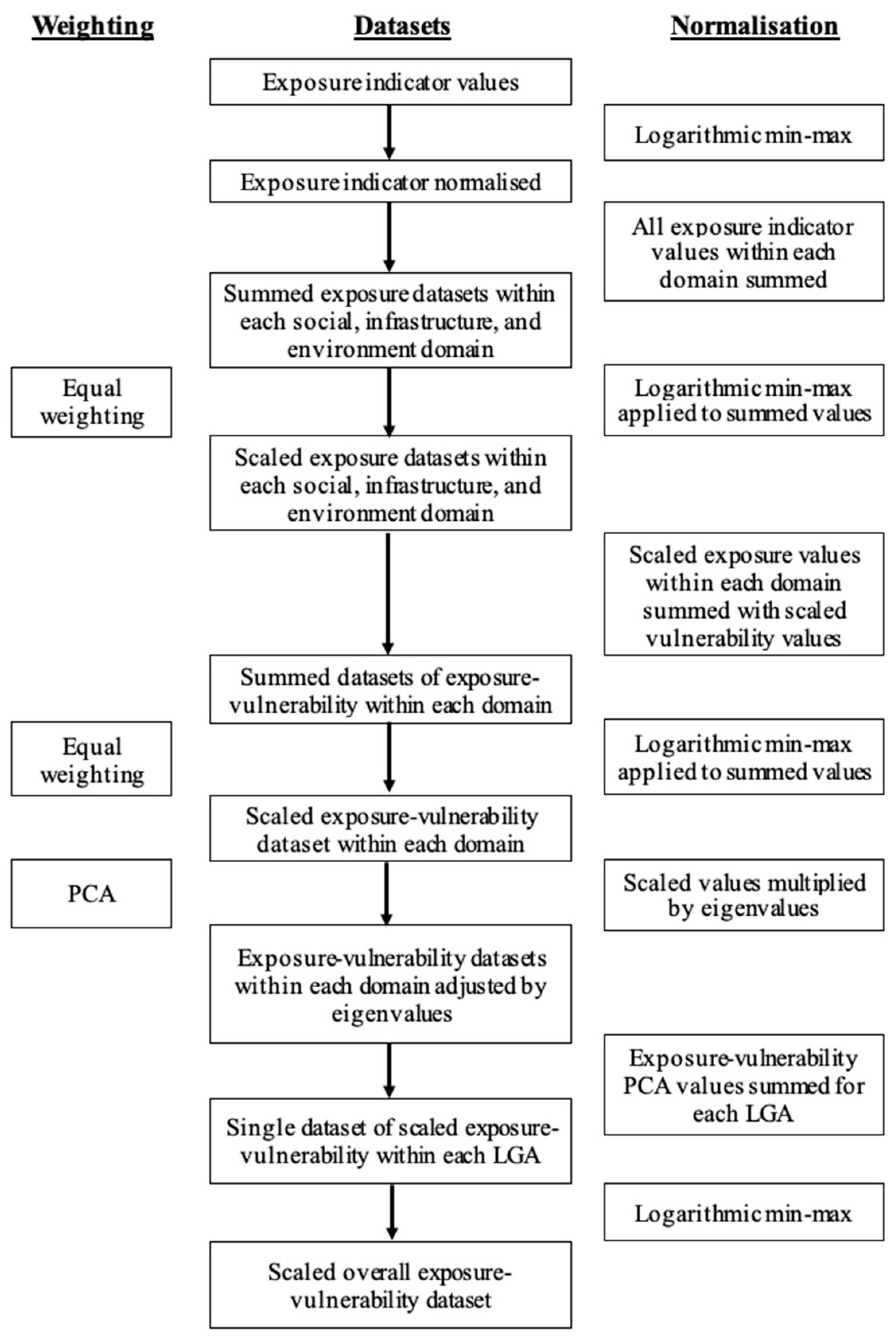
With each indicator’s data converted into a single value for each LGA, the data between the LGAs were then normalised through a logarithmic min–max process, creating a scale from 0 to 1. To then create the social, infrastructure, and environment exposure indices, all normalised exposure indicator datasets within each domain were summed and then again normalised through a logarithmic min–max process to produce a scaled set of values for the indices of social, infrastructure, and environment exposure. An example of this is an exposure dataset within the social domain. This same methodology was performed for vulnerability. From there, the sum of the exposure and vulnerability values within each domain was calculated, and then subjected to another logarithmic min–max calculation to generate a final index for each domain. An example of this is an exposure–vulnerability dataset for the social domain.
This process is visualised in Figure 2, which includes the weighting schemes, the datasets created, and the normalisation techniques applied at each process for the exposure indicators. The same process was utilised for the vulnerability indicators. The blocks representing the steps for the weighting and normalisation columns have been placed between the blocks representing the datasets to explain the weighting and normalisation method used to create the following dataset throughout the methodology.

Figure 2.
Diagrammatic method for weighting and standardising the datasets within this study.
In turn, maps of each indicator, maps of exposure and vulnerability within each domain, and the final exposure–vulnerability index for each domain were produced.
Within each of the social, environment, and infrastructure indices, the equal weighting approach was applied. In this way, each indicator within the indices is seen to be equally critical in the exposure and vulnerability of a region. This approach is commonly used in TC exposure and vulnerability assessments, and although less robust than a PCA, it still provides useful and reliable results. This approach was applied because exposure has two indicators, population density and residential housing, that are highly correlated. When datasets are highly correlated, it implies that they share a substantial amount of information. PCA seeks to maximise the variance in the data, which may result in discarding valuable information that could be crucial for understanding the relationship between the variables when they are highly correlated [56]. By applying PCA, there is a risk of losing valuable information that is present in the original datasets. To ensure that both sides of the exposure and vulnerability indices are methodologically consistent, equal weighting was applied in creating these indices. In summary, the datasets within each domain utilised equal weighting methods, and the overall exposure–vulnerability index links exposure indicators with related vulnerability indicators via PCA. This approach is further explained in Section 2.8.
Charted in Table 4, to assess and map each index, the symbology of the data was graduated into five risk classes: ‘very low’, ‘low’, ‘moderate’, ‘severe’, and ‘extreme’. An equal interval classification mode is most useful when there are only a few data points, so with this study including only six LGAs, this graduation method is appropriate [57]. This method provides an evenly distributed classification scheme, which is effective in displaying and identifying patterns in the data. Furthermore, this mode ensures that each class represents a consistent range of values. Thus, if values for one indicator are all high between the LGAs, this method ensures that these values are all represented through high classes, rather than allocating them into lower classes due to relative comparability. This mode therefore avoids misleading information on comparative values.

Table 4.
Equal Weighting risk classes assigned to values for the overall tropical cyclone exposure–vulnerability index map.
2.6. Exposure–Vulnerability Index
Succeeding the normalisation process and the generation of the social, infrastructure, and environment indices, to prepare the maps for the generation of the overall exposure–vulnerability index, the data were then analysed using a PCA in order to identify the eigenvectors. PCA can be used in this calculation because no two domains are highly correlated. From there, the dataset values were multiplied with their corresponding eigenvalues for each LGA. This provided a table of 3 vector columns, consistent with the 3 domains, for each LGA. Each LGA column was then added before the values were subjected to the logarithmic min–max normalisation process.
These values ranging from 0 to 1 were then inputted into QGIS to create a final exposure–vulnerability index, visualised as a map of the extent and propensity of the assets being exposed and vulnerable to TC damage for each LGA within the study area.
The graduating scheme and symbology applied in the overall exposure–vulnerability index are the same as outlined in Section 2.5.
2.7. Normalisation Technique
The datasets for each indicator were normalised to provide datasets with the same range from 0 to 1, to allow for cross-comparison. The methodology for normalisation includes the logarithmic min–max approach, following Equation (3):
where x is the original data value, x’ is the new normalised value, min(x) is the minimum value in the dataset, and max(x) is the maximum value in the dataset—of which all values must be positive. This approach was utilised because it can rescale the data to the specific range of 0–1 for interpretation and visualisation purposes, and is less sensitive to outliers in the dataset compared to the general min–max normalisation method. With each indicator’s values sharing the same range, cross-comparison and manipulation of the data are simple and feasible, which is of particular interest when indicators come in differing initial scales and values, including numerical versus categorical data. Moreover, this technique is commonly used in risk assessment studies that perform normalisation processes for the dataset [58,59,60].
x’ = (Log10(x) − Log10(min(x)))/(Log10(max(x)) − Log10(min(x)))
2.8. Indicator Weighting
In this study, two approaches for weighting the significance of indicators for the indices were utilised. The first approach is equal weighting. Equal weighting is a common tool that ranks each indicator equally in importance for that study area, for example being utilised in this study [61]. Although research has found this assessment to be reductive and simplifying, a systematic review found that 40% of the papers they reviewed, the largest portion for multi-criteria processing, used this method, primarily due to its methodological simplicity [27].
The second approach is the multivariate technique of PCA, an efficient method for quantifying exposure and vulnerability indicators [32,44,62,63,64,65]. PCA analyses several quantitatively dependent variables to extract important information to identify patterns of similarity between the observations and the variables [66,67]. PCA is a dimensionality reduction technique that transforms a dataset by projecting it onto a new set of orthogonal axes, which are called principal components (PCs). These components are then ordered by the amount of variance they capture in the data. Each indicator influences the creation of the PCs based on the covariance with other indicators, and so indicators exhibiting high variability or correlations with other indicators increase in the propensity to have a larger contribution on the PCs.
3. Results
The five risk classifications for each indicator, outlined in Table 4, have been normalised, making each LGA value relative to the values of the other LGAs within the study area. Thus, an LGA that has been allocated to a lower class does not imply that the exposure or vulnerability is low, but instead that it is low relative to the values in the other LGAs being analysed in this study.
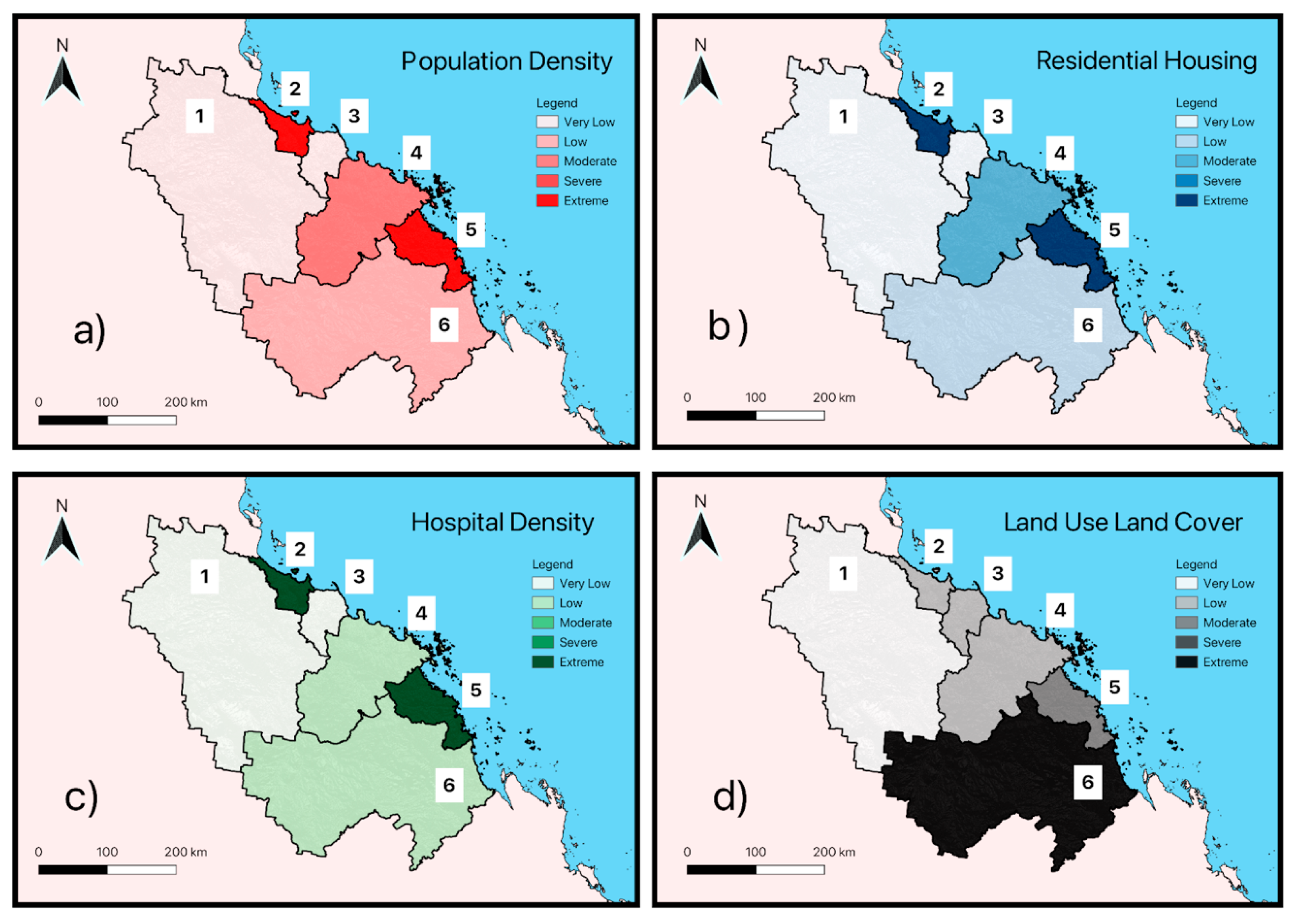
Maps of all four exposure indicators in the designated study area, seen in Figure 3, demonstrate a trend of the most exposed LGAs being the coastal regions, particularly the City of Townsville and Mackay Region, displaying an ‘extreme’ ranking for three of the four indicators. Mackay Region and the City of Townsville only showed a ‘moderate’ and ‘low’ ranking, respectively, for the environmental exposure indicator of LULC.
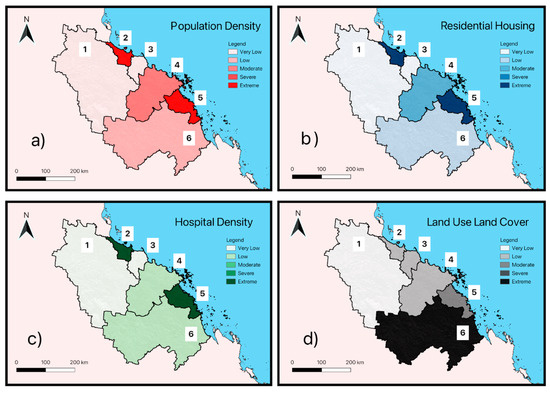
Figure 3.
Maps of tropical cyclone exposure indicators in the six LGAs surrounding TC Debbie landfall, after logarithmic min–max normalisation, with 1 = Charters Towers Region, 2 = City of Townsville, 3 = Burdekin Shire, 4 = Whitsunday Region, 5 = Mackay Region, 6 = Isaac Region (QGIS 3.30 software).
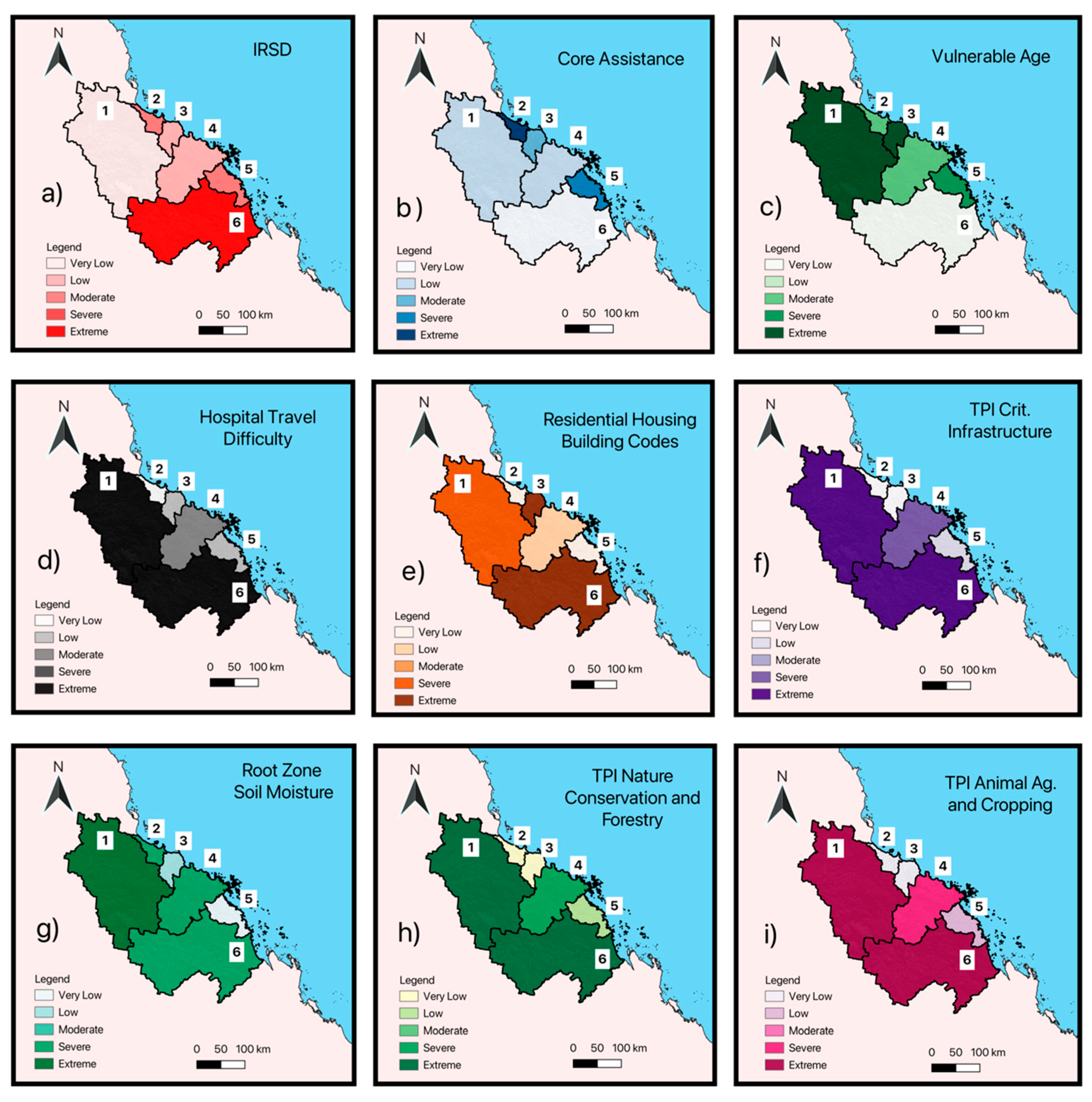
Maps of all nine vulnerability indicators in the designated study area, seen in Figure 4, demonstrate a large variability in the regions with high rankings. The inland LGAs of Isaac Region and Charters Towers Region show trends of high vulnerability, particularly for the infrastructural and environmental vulnerability indicators of residential housing building codes, TPI for critical infrastructure, root zone SM, TPI of nature conservation and forestry, and TPI for animal agriculture and cropping. There is no clear trend in Figure 4a–d, maps of the social vulnerability indicators, with coastal LGAs showing high vulnerability in the core assistance indicator, showing medium vulnerability in the vulnerable age and IRSD indicators, and then showing low vulnerability in the hospital travel difficulty indicator.
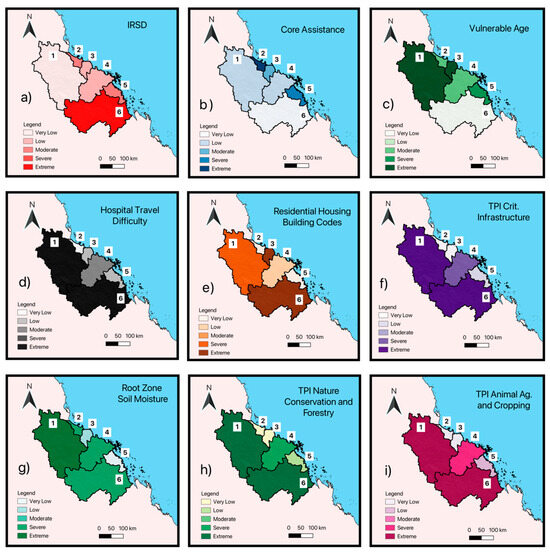
Figure 4.
Maps of tropical cyclone vulnerability indicators in the six LGAs surrounding TC Debbie landfall, after logarithmic min–max normalisation, with 1 = Charters Towers Region, 2 = City of Townsville, 3 = Burdekin Shire, 4 = Whitsunday Region, 5 = Mackay Region, 6 = Isaac Region (QGIS 3.30 software).
Figure 5 combines all social indicators together from exposure and vulnerability to create a map of the social exposure–vulnerability in the designated study area. Figure 5 demonstrates that Mackay Region and the city of Townsville are the most exposed and vulnerable to TC impacts, falling under the ‘extreme’ classification with a normalised value of 1.00 and 0.953, respectively. Whitsunday Region displays a social exposure–vulnerability rating of ‘very low’, showing a value of 0.00. The remaining coastal LGA within the City of Townsville, as well as the inland LGAs of Charters Towers Region and Isaac Region, exhibit a ‘low’ rating. Specifically, the coastal LGA has a value of 0.299, while Charters Towers Region and Isaac Region have values of 0.346 and 0.213, respectively. Overall, the exposure–vulnerability was greater in coastal regions.
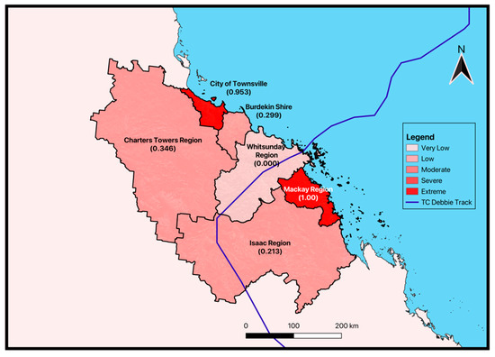
Figure 5.
Map of tropical cyclone social exposure–vulnerability in the six LGAs surrounding TC Debbie landfall, with values after logarithmic min–max normalisation (QGIS 3.30 software).
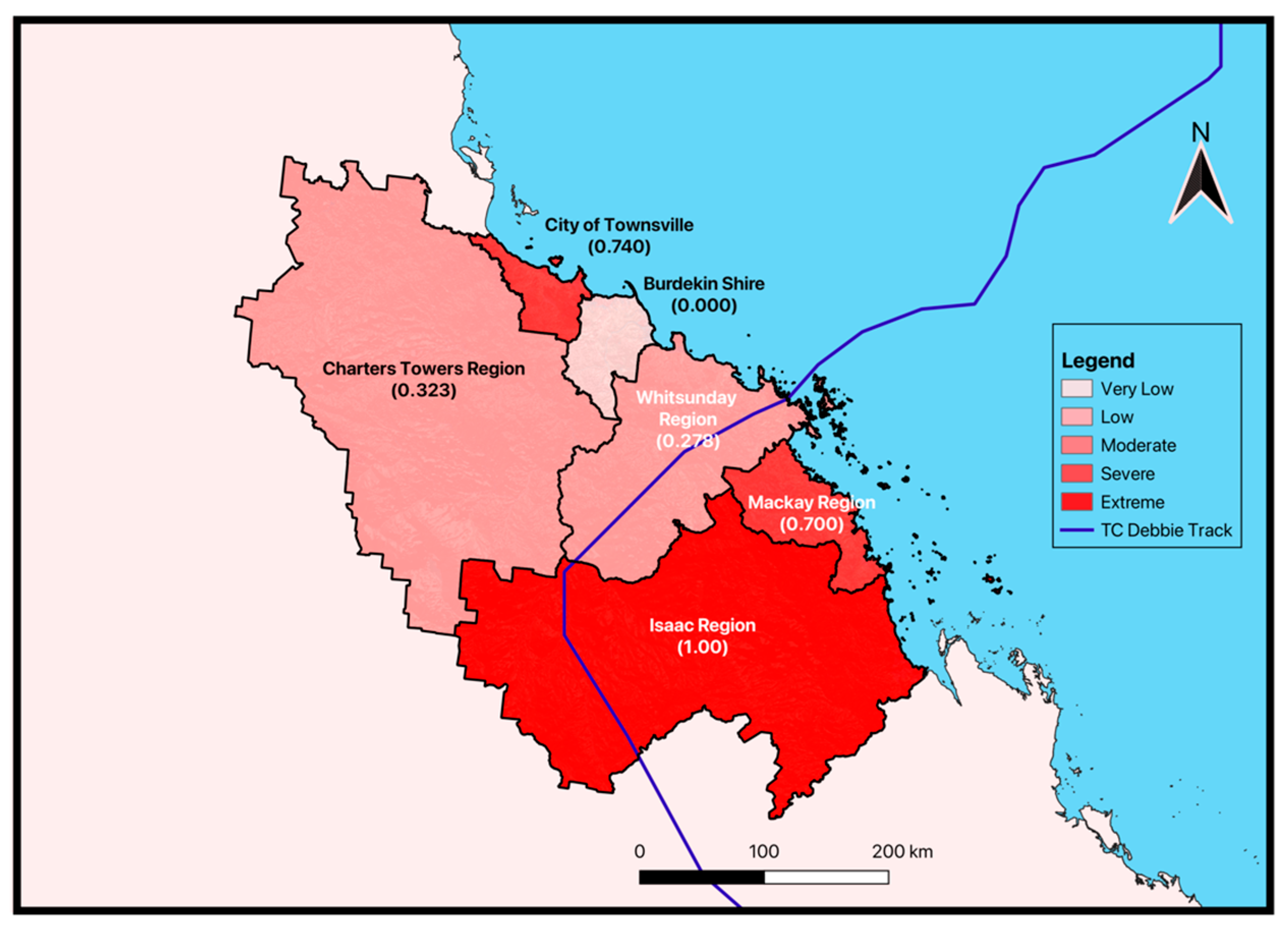
Combining all infrastructure indicators together from exposure and vulnerability, Figure 6 displays a map of infrastructure exposure–vulnerability for the designated study area. Contrasting Figure 5, Isaac Region is the only LGA that has an ‘extreme’ infrastructure exposure–vulnerability ranking (1.00). The City of Townsville and Mackay Region both assume rankings of ‘severe’, with values 0.740 and 0.700, respectively. Unlike other maps where coastal/inland contrast is prevalent, no visible patterns for exposure–vulnerability are displayed within this map. Charters Towers Region and Whitsunday Region both share rankings of ‘low’ exposure–vulnerability, and Burdekin Shire has a ranking of ‘very low’, with a relative exposure–vulnerability of 0.00.
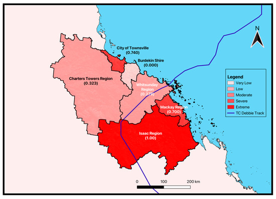
Figure 6.
Map of tropical cyclone infrastructural exposure–vulnerability in the six LGAs surrounding TC Debbie landfall, with values after logarithmic min–max normalisation (QGIS 3.30 software).
Combining all environmental indicators together from exposure and vulnerability, a map of environmental exposure–vulnerability for the designated study area, Figure 7, demonstrates contrasting patterns to that of the social and infrastructural maps seen in Figure 5 and Figure 6. Here, a pattern has been identified where the coastal regions are less exposed and vulnerable to TC damage in this study area than the inland areas. The coastal LGAs of Mackay Region, the City of Townsville, and Burdekin Shire all assume ‘very low’ rankings (0.101, 0.121, and 0.000, respectively). The other coastal LGA of Whitsunday Region receives a ranking and value of ‘moderate’ and 0.542. The more inland LGAs of Charters Towers Region and Isaac Region have ‘extreme’ environmental exposure–vulnerability ratings. Despite some coastal regions within Isaac Region, the large majority of its land mass is inland.
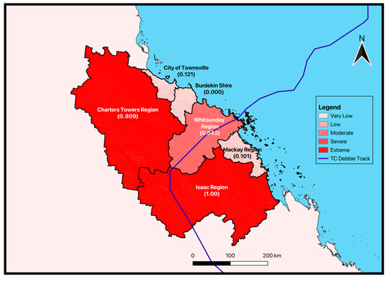
Figure 7.
Map of tropical cyclone environmental exposure–vulnerability in the six LGAs surrounding TC Debbie landfall, with values after logarithmic min–max normalisation (QGIS 3.30 software).
To combine the social, infrastructure, and environment exposure–vulnerability maps to produce the overall map, the values within each map must be multiplied by the eigenvalues generated through PCA. The eigenvalues are found in Table 5. The percentage of variance explained from the first PC in the social domain is 45.28%. This is calculated by summing the total eigenvalues and then dividing the eigenvalue by the total sum. An example for the social domain within Vector 1 is (0.7376/(0.7376 + 0.2744 + 0.6169) × 100%. The vector that explains the most variance is called the first PC. Thus, for the social domain, Vector 1 is the first PC, Vector 3 is the second PC, and Vector 2 is the third PC. For the infrastructure domain, Vector 2 is the first PC representing 58% of the variance in the infrastructure dataset. For the environment domain, Vector 1 is the first PC and explains 39% of the variance in the dataset.

Table 5.
Eigenvalues generated through a PCA, to then be multiplied by the social, infrastructure, and environment values to create the overall exposure–vulnerability map.
Combining the social, infrastructure, and environment exposure–vulnerability maps produces an overall exposure–vulnerability map, seen in Figure 8. The LGAs with an ‘extreme’ rating of exposure–vulnerability from TC impacts are Mackay Region and the City of Townsville, valued at 1.00 and 0.980, respectively. The two inland LGAs of Isaac Region and Charters Towers Region demonstrate a ‘severe’ exposure–vulnerability rating, with values of 0.706 and 0.626, respectively. The other two coastal LGAs, Burdekin Shire and Whitsunday Region, have rankings and values of ‘moderate’ and ‘very low’, 0.217 and 0.000, respectively. In this final map, there is no clear pattern between coastal and inland LGAs. The track map of TC Debbie, displayed in Figure 8, is seen to have made landfall near Airlie Beach within the Whitsunday Region LGA. Despite this, the overall exposure–vulnerability map displays that this LGA has the lowest ranking of exposure and vulnerability from TC impact.
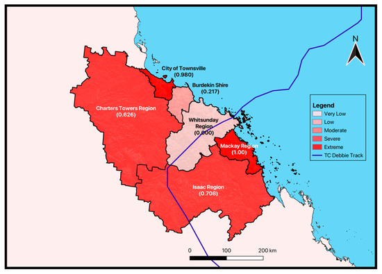
Figure 8.
Map of overall tropical cyclone exposure–vulnerability in the six LGAs surrounding TC Debbie landfall, with values after logarithmic min–max normalisation (QGIS 3.30 software).
4. Discussion
This study aimed to quantify TC exposure–vulnerability through the use of an indicator-based multi-criteria analysis approach, by considering indices that explore societal, infrastructural, and environmental factors associated with exposure and vulnerability. The question driving this investigation asks whether an index-based approach was effective in the assessment of TCs within the eastern coast of Australia. Furthermore, this study has attempted to provide actionable risk data to local decision makers so that specific resilience structures and mitigation strategies can be implemented. The following sections will discuss the findings and reasonings from this study.
4.1. Social Exposure–Vulnerability
In each indicator within this study, the LGA values are relative to the values of the other LGAs within the study area. Thus, given that the methodology has each indicator normalised, LGAs with high exposure or vulnerability might be allocated to a lower class if it is comparatively low compared to the surrounding LGA values.
This study adds value to a field of risk assessment research as it comes from linking exposure indicators with related vulnerability indicators within each domain of social, infrastructure, and environment. This is an improvement from previous literature, including Do and Kuleshov [28], who have also assessed exposure and vulnerability together within the Queensland region, but did so at a lower resolution, did not utilise community-specific indicators, and did not link the indicators together. Through these risk assessment improvements, this study provides more community-specific results that can be used by policy makers to implement specific and contextual mitigation strategies for exposed assets that are also vulnerable to damages from TCs. By using datasets and indicators related to the specific case study of TC Debbie, including the date of impact, this study provides insights through the results being contextual to an event, which can thus be further compared to real damage data from this event to analyse the index’s efficacy. Additionally, including a weighting system for each indicator based on impact improves risk assessment methodology compared to previous studies [28,40] that typically utilised equal weighting mechanisms for indicators.
The social exposure indicator utilised in creating the social exposure–vulnerability index, Figure 5, included population density, and the vulnerability indicators used were IRSD, core assistance, vulnerable ages, and hospital travel difficulty. The map of social exposure (Appendix B) is the same map as the population density exposure indicator map seen in Figure 3a, as this is the only social exposure indicator within this study. This map demonstrates that most populations along the coast have higher TC exposure. Both the City of Townsville and Mackay Region have ‘extreme’ population density exposure, and Whitsunday Region has ‘moderate’ TC exposure. This trend is consistent with Queensland’s urban growth, being in proximity to the central city areas and coastal regions. With urbanisation comes increased development and its associated population growth, and thus higher population exposure in the presence of TC events [68].
The correlation between rapid urban growth and increasing coastal natural hazard risk is well established in the literature [69]. Rapid urban growth and its associated high population density levels within coastal regions is a product of rural–urban migration and environmental urban fertility [69,70,71]. However, rapid urbanisation puts pressure upon water resources, increases deforestation, and degrades coastal environments, all of which combine to increase natural hazard risk [72]. The process of deforestation undertaken for urban development purposes produces extensive water runoff and can obstruct city drainage systems, resulting in storm water flooding [73]. However, these compounding factors can be avoided through better land and infrastructure management [73].
It is important to note that this study utilised population density as a social exposure indicator as opposed to alternative methods such as absolute resident population because population density can normalise between differently sized study regions. Population density data were taken from the Statistical Area 2 (SA2) scale, similar in size to suburbs, and then averaged into the LGA scale. Thus, data might have been lost in the process of rescaling, which could have reduced the reliability of the results. Nevertheless, this method was most appropriate for the scale and methodology of this study, and population density at an LGA scale still provided suitable results to draw upon.
The exposure indicator of population density is directly linked to the social vulnerability indicators. The inland LGA of Charters Towers Region has an ‘extreme’ ranking for two of the four social vulnerability indicators: vulnerable age and hospital travel difficulty. Thus, the population density exposure map in Figure 4a contrasts the social indicator TC vulnerability maps (Figure 4c,d), which demonstrates high levels of social vulnerability within the inland LGA of Charters Towers Region. This can be further explained through Appendix C to demonstrate the social TC vulnerability of this LGA. Hence, the ability to travel to a hospital, compounding the population density of people aged below 15 or above 65, makes this inland region highly vulnerable to social damages from TC impacts, such as flooding or severe winds.
It should also be noted that hospital travel difficulty measures the crow’s flight distance. A more expansive analysis would make use of the road network and population density as a consideration when measuring distance from residential housing to hospitals. This would require finding the shortest route within the road network from each residential house to each hospital within the constraints of the LGAs, and then averaging these values across the region. Through the crow’s flight method, travel difficulty was heavily influenced by land mass and the number of hospitals in each LGA, rather than taking into account the road network, population density, and infrastructure available to access health facilities. Resultantly, as seen in Figure 4d, the LGAs with the greatest travel difficulty were seen as the two largest LGAs, with ‘extreme’ and ‘severe’ rankings for Charters Towers Region and Isaac Region, respectively.
This limitation is of particular importance in circumstances where roads are impacted by fallen power lines or trees. In these cases, vulnerability can be greatly increased when there is a single road in and out of a community when reaching a hospital, as the accessibility of these critical services can be severely reduced [74]. Therefore, for this reason, it is crucial to know whether various options exist to travel to the hospital, and the fastest route of transportation.
Despite this indicators’ limitation, crow’s flight distance can be a useful proxy for road-based distances and this result is consistent with the health-care access data in the literature [75]. This is particularly true in areas where road data are unavailable, or where road conditions are poor and undergoing constant maintenance. Additionally, during TC events, heavy rainfall may make dirt roads impassable. In these circumstances, the data are not truly reflective of the actual road conditions, making the crow’s flight method a judicious approach [76,77].
Additionally, this result is supported regarding that access to health-care services in rural settings is limited [75]. Typically, the proximity to hospitals and number of hospitals within rural settings are minimal in comparison to coastal, urbanised areas. Through urbanisation, population density and associated development has been heightened in coastal LGAs. Thus, consistent with the results found in Figure 4d, the number of hospitals and the proximity of residential houses to the hospitals are greater in the coastal LGAs where the difficulty of hospital travel is least extreme, ranging from ‘moderate’ to ‘very low’.
Although no clear trends can be made within Figure 4c, the vulnerable age group indicator contributes to shaping Charters Towers Region’s vulnerability and so is crucial in determining the overall vulnerability of its population. People found within the two age groups of below 15 or above 65 have heightened vulnerability through their limited mobility and cognitive ability, impeding on their capacity to respond and cope with the impacts of a TC [78]. Children below the age of 15 may be unable to effectively communicate their needs or comprehend the severity of the event [79]. Simultaneously, individuals who are aged 65 or older may experience greater difficulties with regards to evacuation procedures, accessing medications, or accessing vital emergency services [80]. Furthermore, these age groups are more vulnerable to physical impacts from TCs through their multi-hazards of storm surges, destructive winds, infrastructure collapses, and heavy rainfall.
Interestingly, the IRSD indicator shows an ‘extreme’ classification for Isaac Region (Figure 4a). Areas with low IRSD scores indicate a high percentage of people with a state household income between AUD 1 and AUD 25,999 per year, or a high percentage of people in the labour force being unemployed. Hence, Isaac Region’s high IRSD value indicates a large social disadvantage. This contrasts the social exposure–vulnerability TC map in Figure 5 where Isaac Region has a ‘low’ ranking, which can be explained by its lower rankings in population density, core assistance, and vulnerable age.
A typical social vulnerability indicator for TC risk assessments is the unemployment rate [3]. However, one of the variables in IRSD is the percentage of people unemployed in the labour force (Appendix A). To avoid doubling of indicators and skewing the data, the individual unemployment indicator has been omitted from this study and was instead utilised as a variable within the IRSD indicator.
Seen in Figure 4b, a substantial impact causing the vulnerability of the City of Townsville is its ‘extreme’ ranking from the core assistance indicator. The relationship between increased core assistance and increased vulnerability is credited to the mobility impairment, which is critical in evacuation protocols during an emergency. Additionally, the medical needs of people within the CANA group during a TC event may necessitate access to critical resources such as medication, electricity, and specialised equipment. Failure to meet these needs can result in life-threatening consequences, augmenting their vulnerability in such events [81].
Figure 5 combines all social indicators to generate a social TC exposure–vulnerability map, where the coastal LGAs of Mackay Region and the City of Townsville have an ‘extreme’ classification. This indicates that for the assets that are exposed to a TC, they are also extremely vulnerable to damage. This is in alignment with the population density of the LGAs, with the City of Townsville having the highest population density, followed by Mackay Region. Both coastal regions being ranked as ‘extreme’ for overall social exposure–vulnerability from TC gives insight that not enough efforts have been put in place to improve their social resilience from natural hazard risks.
Particularly being coastal, the exposed assets in combination with the vulnerability of these assets are truly at risk of damage when triangulating the third risk factor of hazard. TCs are strongest and pose the greatest risk to humans when they make landfall at the coast, including the impacts of coastal hazards like storm surges [82]. So, LGAs closer to the ocean have a greater propensity to damage.
Whitsunday Region had the lowest social exposure–vulnerability ranking of ‘very low’ with a value of 0.00. This opposes the above findings and previous literature claiming that coastal regions are the most exposed and vulnerable to water-based natural hazards. However, this value is consistent with the results, where as seen in Figure 3a, Whitsunday Region has a population density ranking of ‘very low’. Additionally, Figure 4a,b show Whitsunday with a ‘low’ ranking for both IRSD and core assistance, and Figure 4c,d show this LGA to have a ‘moderate’ ranking for both vulnerable age groups and hospital travel difficulty.
Albeit, Whitsunday was the LGA in which TC Debbie made landfall and travelled through before reaching Isaac Region. Whitsunday faced various challenges from this TC; however, its social calamity was likely less severe through its low population density, its strong population economic status, the health of the population, and their access to health-care services [41]. It is therefore postulated that if TC Debbie made landfall in either the City of Townsville or Mackay Region, the population within either LGA would have faced more severe social challenges through the TCs’ damage.
With Mackay Region and the City of Townsville having the lowest social exposure–vulnerability rankings, mitigation strategies should primarily be focused within these two LGAs to reduce the risk of impacts from TCs. Examples of this could include improving and expanding the social assistance mechanisms in place by local councils for people in need of daily support. This would aid marginalised people to avoid harm from TC events. Moreover, there should be a focus on providing public TC shelters, public temporary housing, public evacuation options, and foodbanks. In the case where a rapid evacuation is needed, the ability to safely house people is critical to the social resilience of the population. Additionally, with high classes of IRSD for both LGAs, the government could instigate more regimented governmental financial assistance and employment opportunities for people living in a low socio-economic status. Through this, low-income people are more likely to increase their financial stability, which can allow them to afford better resilience infrastructure for their homes, improved modes of transport, and increased ability to financially support medical assistance and disability aid.
4.2. Infrastructure Exposure–Vulnerability
The exposure indicators utilised in creating the infrastructure exposure–vulnerability index included residential housing and hospital density, and the vulnerability indicators were residential housing building codes and TPI for critical infrastructure. In the infrastructure domain, the exposure indicators were highly influential in the final index because of the strong correlation between the two indicators. There is a strong link between the number of residential housing and the number of hospitals that exist in the surrounding geographical location [83]. There is typically a strong positive relationship, where with more residential housing, indicative of a high population, the hospital density increases [3]. As a result, Figure 3b,c show similar trends where LGAs have a similar infrastructure exposure ranking for both indicators. Both the City of Townsville and Mackay Region have the highest ranking of ‘extreme’, and Charters Towers Region has the lowest ranking of ‘very low’.
The infrastructure vulnerability indicator of building codes relates directly to the exposure indicator of residential housing, as the 1980s’ building code strictly addressed residential housing [51]. The prospect of vulnerability from residential housing building codes was highest for the LGAs of Isaac Region and Burdekin Shire with rankings of ‘extreme’ (Figure 4e). The two most populated and urbanised LGAs, Mackay Region and the City of Townsville, both held rankings of ‘very low’, indicating that residential housing in these LGAs is least vulnerable to TC damage. Charters Towers Region, the other inland LGA, had a ranking classification of ‘severe’.
This is consistent with the prospect that coastal, highly urbanised areas have increased development, and larger economic bases and financial resources [84]. With that comes financial liberty to invest in the construction of new homes with the updated building codes, resulting in a higher proportion of building resilience. The three least urbanised LGAs with the lowest population density have the highest proportion of residential houses constructed prior to the 1980s. Thus, these LGAs are more vulnerable to impacts from TC severe winds that can ultimately apply great sums of pressure to the roof, with the ability to lift the house or its infrastructure from its foundation.
Additionally, urban areas tend to have better access to information and resources compared to rural areas [85]. Thus, there is a likelihood that the information of the new building codes and the importance it has on TC damage disseminated through the urbanised areas faster. So, this could have motivated house owners, builders, and local authorities in urban areas to prioritise compliance with the updated building codes.
Finally, coastal areas often face higher degrees of TC damage than inland areas [82]. Thus, there is a prioritisation of these coastal regions to invest in TC risk reduction, including the construction of new housing. This increases resilience to the potential damages from TCs with the updated building codes.
Unsurprisingly, the LGAs with the highest ranking for hospital density are again the coastal regions of Mackay Region and the City of Townsville—consistent with the relative population densities of the LGAs in this study area. There is a correlation between population density and the number of critical infrastructure buildings, including hospitals, within Queensland [28]. This correlation is commonly accepted as infrastructure is built to address the needs of the population. Particularly, hospitals are placed to cater for a relative portion of the region and their population, with hospitals housing four beds per 1000 citizens in Australia [86].
Linked directly to hospital density is the infrastructure vulnerability indicator of TPI for critical infrastructure. Critical infrastructure in this indicator includes hospitals, alongside other vital services including, but not limited to, health-care services, factories, and residential housing. Seen in Figure 4f, the TPI for critical infrastructure is ‘extreme’ for the two inland LGAs of Isaac Region and Charters Towers Region, and ‘severe’ for Whitsunday Region.
The vulnerability of critical infrastructure intersecting low TPI values can be explained by the mountainous regions following the Great Dividing Range within eastern Australia. The Great Dividing Range is a mountain terrain on the east coast of Australia, stretching from Dauan Island in the Torres Strait to western Victoria, comprising a series of plateaus and low mountain ranges. With mountainous terrain comes high TPI values through large topographic dips and increases. Thus, the vulnerability of critical infrastructure within this region will be higher, as exposed assets are more likely to experience flooding and damage from TCs when in a low TPI classification.
The TPI approach reveals more about the topographical vulnerability of a region than elevation, a more common indicator within TC risk assessments [27,87]. Although elevation might be low, which is typically indicative of high vulnerability, the surrounding elevation might also be low, and so the impact on that specific region will be decreased. Therefore, integrating the slope and elevation together in generating a TPI indicator serves as a more reliable proxy for identifying areas of vulnerability.
An indicator that could be utilised in future studies includes an additional infrastructure vulnerability indicator that analyses the height of the first floor for critical infrastructure. Although some hospitals might have a low TPI and thus a higher vulnerability to TC damage, if their first floor has a high floor level above the ground, this would reduce the risk of flooding and thus infrastructural damage.
When combining infrastructure exposure and vulnerability, seen in Figure 6, the only LGA with a classification of ‘extreme’ is Isaac Region. The two coastal LGAs of Mackay and the City of Townsville have rankings of ‘severe’, and then both Charters Towers Region and Whitsunday Region have rankings of ‘low’. Although Burdekin Shire had an ‘extreme’ ranking for residential housing building codes, its overall infrastructure exposure–vulnerability ranking was ‘very low’ due to its ‘very low’ ranking for residential housing, hospital density, and TPI in critical infrastructure (Figure 3b,c and Figure 4f).
Thus, to improve the TC resilience for these regions, the number of hospitals and health-care services could be increased within the inland LGAs and placed in population-dense regions. This will secondarily improve the hospital travel feasibility in these regions. Furthermore, local councils could encourage construction of residential housing that incorporates newer building codes to combat and withstand TC damage. Additionally, for critical infrastructure assets in low-TPI settings, additional building codes could be implemented to ensure that the height of the first floor is above a specific level to minimise TC damage. These decisions would ultimately minimise the potential infrastructural damage that comes with TC risk.
4.3. Environment Exposure–Vulnerability
The exposure indicator utilised in creating the environment exposure–vulnerability index was LULC, and the vulnerability indicators were root zone SM, TPI for nature conservation and forestry, and TPI for animal agriculture and cropping. LULCs were apportioned into eight classifications (Table 3), and each classification was graduated based on their relationship with prospective human-focused damage from TCs. Evaluating LULC as an exposure indicator is critical because varying LULCs contribute to TC exposure to different extents. Ultimately, the damage assumed by the community is contingent on what LULCs are exposed to TCs.
The valuing system for each LULC can be deemed subjective. However, this valuing system was conducted based on the literature surrounding TC events and an LULC’s pertinence in a community’s resilience to such events. As an example, cropping was weighted as 0.7 because it is one of the most critically exposed and vulnerable environmental assets to TC events. Notably, TC Debbie significantly impacted cropland, where Bowen, one of the largest cropping regions in the eastern coast of Australia, had its vegetable industry damaged by an estimated AUD 100 million [88]. Conversely, water bodies were weighted as 0.1 because, with direct relationships with human lives and livelihoods, this classification’s exposure status is relatively unimportant in a TC event.
Seen in Appendix D, animal agriculture and cropping consumed the most geographical space in the study area, of which they have a high weighted value for exposure. Given that there is large human-based liability that comes with TC damage to cropland and livestock, the risk of TC damage is heightened for regions with this LULC. In the LGAs of Isaac Region, Charters Towers Region, and Whitsunday Region, animal agriculture and cropping were vast in landmass, relative to the other LGAs in the study area. Seen in Figure 3d, Isaac Region had an exposure LULC ranking of ‘extreme’. The next highest classification was by Mackay Region with a ‘moderate’ ranking. Isaac Region has the highest amount of environmental assets exposed to potential TC damage because it is majorly inland with large portions of land designated to cropping and animal agriculture (Appendix D).
Linked directly to the LULCs’ exposure environment indicator are the vulnerability indicators. Seen in Figure 4g, root zone SM was seen to be ‘extreme’ within Charters Towers Region, and then ‘severe’ for Isaac Region, Whitsunday Region, and the City of Townsville. Root zone SM followed a similar pattern to TPI for critical infrastructure, seen in Figure 4f. SM has been shown, through current literature, to largely influence the vulnerability of communities impacted by TCs [89,90,91]. Saturated soils cannot absorb additional rainfall from the TC, generating more rapid and severe flooding [92]. As a result, the region impacted is more likely to experience events including landslides through unstable soil. Soil types with high infiltration consist of larger pore spaces [93]. The larger spacing within the root soil creates deposits that readily accept water. The saturated hydraulic conductivity of low-infiltration soil contains smaller pore spaces between soil aggregates, leaving less room for infiltration [16]. These soils are expected to absorb less water, resulting in runoff remaining on the surface and an increased chance of environmental harm from TC-related flood events.
Additionally, high soil moisture can impact the stability of trees through influencing the depth and integrity of root systems. In conjunction with strong winds, TCs can uproot trees in areas of high soil moisture due to the soil’s lack of stability and cohesion, whereas in areas with dry soils, trees are less susceptible to wind damage [94].
Seen in Figure 4g, the root zone SM is larger in inland regions. Rural areas consist of largely non-interfered soils compared to anthropogenically changed, urbanised areas [95]. As a result, the underdeveloped nature of the rural areas yields more pore space, increasing organic matter and biomass. The biomass enters the ground, primarily through the root systems, assisting in the aggregation of the soil and increasing pore space [16]. This is consistent with the results produced in Figure 4g, with the inland LGA of Charters Towers having ‘extreme’ root zone SM, and the heavily inland regions of Whitsunday Region and Isaac Region displaying ‘severe’ rankings for this indicator.
Utilising TPI below −24, being the two lowest TPI classifications, finding areas of TPI overlapping with nature conservation and forestry and with animal agriculture and cropping shows similar patterns (Figure 4h,i). Both maps display Isaac Region and Charters Towers Region with an ‘extreme’ ranking, and then Whitsunday Region with a ‘severe’ classification. The remaining coastal regions have ‘very low’ to ‘low’ rankings. This is consistent with the aforementioned Great Dividing Range locations, where inland regions are more mountainous and so experience larger slope extremities between a specific location and its surrounding environment. Additionally, as seen through the LULCs’ map in Appendix E, the inland regions consist of the most nature conservation and forestry areas, and animal agriculture and cropping. This is due to the urbanisation trends seen in coastal regions within Australia, removing these natural and agricultural environments to create space for residential housing and city infrastructure. With increased amounts of nature conservation, forestry, animal agriculture, and cropping, there is a greater propensity for overlap between low TPI values and these areas.
Combining the environment exposure and vulnerability indicators together, a final map is created, seen in Figure 7. Figure 7 denotes the inland regions of Isaac Region and Charters Towers Region with ‘extreme’ environmental exposure–vulnerability, displaying normalised values of 1.00 and 0.81, respectively. The three coastal regions of Mackay Region, Burdekin Shire, and the City of Townsville are all ranked as ‘very low’, with values of 0.10, 0.00, and 0.12, respectively. Whitsunday Region has a ‘moderate’ ranking with a value of 0.54. Although Whitsunday Region is also coastal, a large portion of its land mass is, in fact, inland. Thus, the ‘moderate’ ranking for this LGA is logical. The disparity in environment exposure–vulnerability results holds true with regions that are least urbanised being the most exposed and vulnerable to environmental harms from TCs.
To mitigate against the harms of prospective TC damage, local decision makers and stakeholders should consider mechanisms to protect these environmental assets. Examples of solutions could include drainage water management through subsurface tile drainage to protect cropping and animal agriculture from floods, and water gates to help farmers protect their crops and livestock from floodwater [96].
4.4. Overall Exposure–Vulnerability Index
The values from the social, infrastructure, and environment exposure–vulnerability indices, found in Figure 5, Figure 6 and Figure 7, were then multiplied by the PCA values found in Table 5 to generate the overall exposure–vulnerability map (Figure 8) for the designated study area. PCA was utilised to generate this final map for various reasons, primarily including dimensionality reduction and an objective weighting scheme. PCA assists in reducing the dimensionality of the data by transforming the original variables into a new set of uncorrelated variables, the PCs. Additionally, PCA assigns weights to each PC based on their contribution to the overall variance of the data. The first PC accounts for the most significant amount of variance, followed by the second and then the third. The weights generated by PCA specify the relative importance of each PC in explaining the data. The PCA weights thus reflect the importance of each of the social, infrastructure, and environment indices in determining the overall exposure–vulnerability index.
Within the PCA eigenvalues, two of the domains had their first PCs representing less than 50% of the variance in the dataset. This infers that a large portion of the variance has not been captured by these components. A potential reason for this was inherent complexity, where the dataset could have had a high degree of complexity and inherent variability that was not captured effectively by a small number of PCs [97]. As an example, in the IRSD indicator, there are various inputs, seen in Appendix A, which makes this indicator complex. The spread of data within this indicator can therefore be unclear in how it interacts with other input datasets, generating greater variability and uncertainty in the final dataset.
Utilising the eigenvectors to generate the final exposure–vulnerability map, the two LGAs with an ‘extreme’ ranking are Mackay Region and the City of Townsville, with normalised values of 1.00 and 0.980, respectively. Thus, these two regions are the most exposed and vulnerable to TCs within this study area. Following this, Isaac Region (0.708) and Charters Towers (0.626) had a ‘severe’ ranking. Burdekin Shire (0.217) and Whitsunday Region (0.000) fell into the rankings of ‘moderate’ and ‘very low’, respectively.
These results are validated by the impacts felt by the communities within Mackay Region, where destructive winds and torrential rain resulted in significant damage to homes, infrastructure, and agriculture across the region [50]. Additionally, major flooding critically impacted many communities within this region [50]. However, both in Mackay Region and Whitsunday Region, over 90 percent of the community service respondents stated that they were satisfied with the speed and proficiency of the decision makers’ responses to the event and the time in which they could return home after being evacuated [50].
Importantly, the value of 0.000 for exposure–vulnerability associated with Whitsunday Region can appear misleading. Given all values have been normalised and made relative to the other LGAs in the study area, one region will have the value of 0.000 and another region a value of 1.00. Hence, this value does not infer that Whitsunday Region has no exposed assets or that the exposed assets are protected from damage. Whitsunday Region, being a coastal region on the eastern coast of Australia, has fallen victim to damage from natural hazards, including TC Debbie [50]. When combining exposure and vulnerability with hazard, this region has a greater propensity to risk from TCs than many inland areas that are likely to never experience damage from such events [87]. Thus, protocols and resilience strategies are still required to ensure that such a region curtails the possibility of either societal, infrastructural, or environmental damage from TCs.
The overall exposure–vulnerability index displays largely high rankings for the LGAs, with two regions having their assets exposed and vulnerable to an ‘extreme’ extent, followed by two regions being ‘severe’, and then another being ‘moderate’. Thus, it is clear that this is a highly exposed and vulnerable region to the threats and damages of TCs, and so ultimately mitigation strategies are required to reduce the damages and ultimate loss of lives and livelihoods from such events.
In earlier studies [98,99], combined indices for coastal risk assessment have been developed. However, in this study, specifically focused on TCs, each exposure indicator is linked to a related vulnerability indicator, rather than having a list of exposure and vulnerability indicators with some relationship as in [100,101]. Through the methodology developed in this study, decision makers have a better understanding of specific exposed assets and their vulnerability to TC-related damages.
For this methodology to be transferred to other study areas, particularly those more vulnerable to the damages of TCs, there is a need to select community-specific indicators. These include datasets that directly relate to the exposed assets and the vulnerability of such assets within the community and study area being assessed. An example of this could include selecting the number of informal settlements within the coast of Fiji to assess the vulnerability of infrastructure in this Pacific-island country [102]. When applying this methodology to a global lens, exposure and vulnerability would need to be combined with a hazard model [21]. Examples of hazard models that can be utilised within a comprehensive TC risk assessment are through Random Forest Machine Learning techniques to assess flooding hazard [100] or a Variable Enhanced Bathtub Model to assess storm surge hazard [101].
5. Conclusions
To improve TC risk assessments, this study developed an exposure–vulnerability index, utilising the study area of TC Debbie in the six LGAs surrounding landfall. Therefore, local decision makers are provided with insight into appropriate action to reduce future losses of human lives and livelihoods. This study could serve as a proof-of-concept methodology for other TC-prone regions.
It was found that the LGAs most exposed and vulnerable to TC damage were the two coastal LGAs of Mackay Region and the City of Townsville, receiving exposure–vulnerability values of 1.00 and 0.97, respectively. This is due to a combination of societal factors including a large need for core assistance, highly vulnerable age groups, a high proportion of residential housing with antiquated building codes, and a high population density.
The results from this study provide a valuable contribution to the discussion of TC management in Australia and abroad. The linked exposure and vulnerability indicators utilised within this study are suitable proxies in describing TC-prone landscapes of Australia’s eastern coastal regions. Given that this index-based technique is simple and transferable to other regions, a similar risk assessment could be conducted in other areas concerned of TC damage. Insight from this proof of concept can also assist TC mitigation and adaptation in other TC-prone areas outside of this study area, which is bolstered by the openly accessible nature of an index-based methodology.
This study adds value to the TC risk assessment scientific landscape through linking exposure and vulnerability indicators, and having them ranked using a PCA approach, within the study area of impacted LGAs surrounding the landfall of TC Debbie in the eastern coast of Australia.
Ultimately, this research can help relevant decision makers and stakeholders to gain better insight into TC risk management for disaster risk reduction, by introducing policy that relates closely with the exposed and vulnerable assets within their community. In a landscape where TC intensity is continually increasing in the presence of anthropogenic climate change, the replicable and scalable TC risk assessment scoped by this research will serve as a meaningful and proactive method for TC mitigation and adaptation. It is recommended that the methodology used for this study is considered as a potential framework for future index-based TC assessment approaches.
Author Contributions
Conceptualization, K.B. and Y.K.; methodology, K.B.; software, K.B.; validation, K.B.; formal analysis, K.B.; investigation, K.B.; resources, Y.K.; data curation, K.B.; writing—original draft preparation, K.B.; writing—review and editing, K.B. and Y.K.; visualization, K.B.; supervision, Y.K.; project administration, Y.K.; funding acquisition, Y.K. All authors have read and agreed to the published version of the manuscript.
Funding
This research received no external funding.
Data Availability Statement
Data are contained within the article.
Acknowledgments
The authors express sincere gratitude to colleagues from the Climate Risk and Early Warning Systems (CREWS) team at the Australian Bureau of Meteorology and Monash University for their helpful advice and guidance.
Conflicts of Interest
The authors declare no conflict of interest.
Appendix A. List of All 16 Variables That Are Used to Create the IRSD Index. All Variables Are Indicators of Disadvantage
- INC_LOW: % of people with stated household equivalised income between AUD 1 and AUD 25,999 per year
- CHILDJOBLESS: % of families with children under 15 years of age who live with jobless parents
- NONET: % of occupied private dwellings with no internet connection
- NOYEAR12ORHIGHER: % of people aged 15 years and over whose highest level of education is Year 11 or lower
- UNEMPLOYED: % of people (in the labour force) who are unemployed
- OCC_LABOUR: % of employed people classified as Labourers
- LOWRENT: % of occupied private dwellings paying rent less than AUD 215 per week (excluding AUD 0 per week)
- ONEPARENT: % of one-parent families with dependent offspring only
- DISABILITYU70: % of people under the age of 70 who have a long-term health condition or disability and need assistance with core activities
- SEPDIVORCED: % of people aged 15 years and over who are separated or divorced
- OCC_DRIVERS: % of employed people classified as Machinery Operators and Drivers
- OCC_SERVICE_L: % of employed people classified as low-skill Community and Personal Service workers
- NOCAR: % of occupied private dwellings with no cars
- OVERCROWD: % of occupied private dwellings requiring one or more extra bedrooms
- NOEDU: % of people aged 15 years and over who have no educational attainment
- ENGLISHPOOR: % of people who do not speak English well
Appendix B. Map of Tropical Cyclone Social Exposure in the Six LGAs Surrounding TC Debbie Landfall, with Values after Logarithmic Min–Max Normalisation (QGIS 3.30 Software)
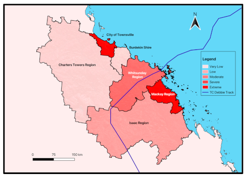
Appendix C. Map of Tropical Cyclone Social Vulnerability in the Six LGAs Surrounding TC Debbie Landfall, with Values after Logarithmic Min–Max Normalisation (QGIS 3.30 Software)
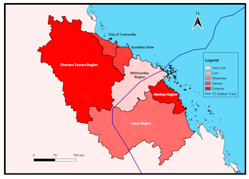
Appendix D. Map of Land Use Classifications of Animal Agriculture and Cropping in the Six LGAs Surrounding TC Debbie Landfall (QGIS 3.30 Software)
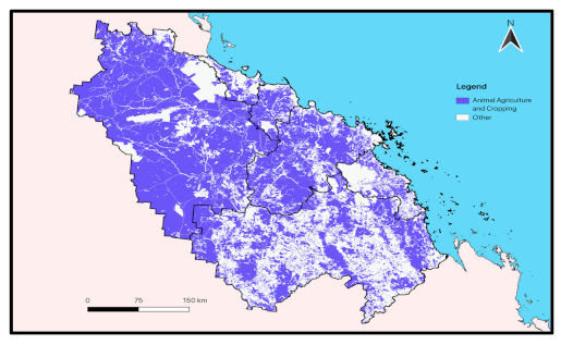
Appendix E. Map of All Eight Land Use Classifications in the Six LGAs Surrounding TC Debbie Landfall (QGIS 3.30 Software)
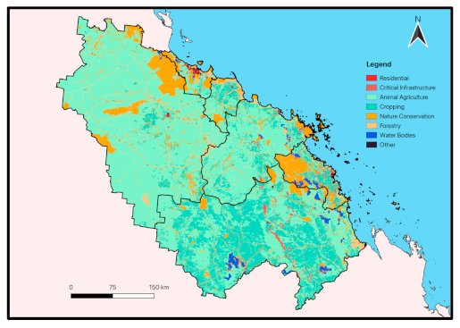
References
- UNDRR. Hazard Definition and Classification Review. I. S. Council. 2020. Available online: https://council.science/wp-content/uploads/2020/06/UNDRR_Hazard-Report_DIGITAL.pdf (accessed on 14 September 2023).
- Turton, S.M. Securing Landscape Resilience to Tropical Cyclones in Australia’s Wet Tropics under a Changing Climate: Lessons from Cyclones Larry (and Yasi). Geogr. Res. 2012, 50, 15–30. [Google Scholar] [CrossRef]
- Do, C.; Kuleshov, Y. Multi-Hazard Tropical Cyclone Risk Assessment for Australia. Remote Sens. 2023, 15, 795. [Google Scholar] [CrossRef]
- Yeasmin, A.; Chand, S.; Turville, C.; Sultanova, N. Detection and verification of tropical cyclones and depressions over the South Pacific Ocean basin using ERA-5 reanalysis dataset. Int. J. Climatol. 2021, 41, 5318–5330. [Google Scholar] [CrossRef]
- Chand, S.S.; Dowdy, A.J.; Ramsay, H.A.; Walsh, K.J.E.; Tory, K.J.; Power, S.B.; Bell, S.S.; Lavender, S.L.; Ye, H.; Kuleshov, Y. Review of tropical cyclones in the Australian region: Climatology, variability, predictability, and trends. Wiley Interdiscip. Rev. Clim. Change 2021, 12, e686. [Google Scholar] [CrossRef]
- Kim, H.M.; Webster, P.J.; Curry, J.A. Impact of Shifting Patterns of Pacific Ocean Warming on North Atlantic Tropical Cyclones. Science 2009, 325, 77–80. [Google Scholar] [CrossRef]
- Dare, R.A.; Davidson, N.E.; McBride, J.L. Tropical Cyclone Contribution to Rainfall over Australia. Mon. Weather Rev. 2012, 140, 3606–3619. [Google Scholar] [CrossRef]
- Kuleshov, Y. “Climate Change and Southern Hemisphere Tropical Cyclones” International Initiative: Twenty Years of Successful Regional Cooperation. In Climate Change, Hazards and Adaptation Options. Climate Change Management; Filho, W.L., Nagy, G., Borga, M., Muñoz, D.C., Magnuszewski, A., Eds.; Springer: Berlin/Heidelberg, Germany, 2020; pp. 411–439. [Google Scholar] [CrossRef]
- ICA. Climate Change Impact Series: Tropical Cyclones and Future Risks [Impact Series]. Insurance Council of Australia. 2021. Available online: https://insurancecouncil.com.au/wp-content/uploads/2021/12/2021Nov_Tropical-Cyclones-and-Future-Risks_final.pdf (accessed on 14 September 2023).
- Coates, L.; Haynes, K.; Radford, D.; D’Arcy, R.; Smith, C.; van den Honert, R.; Gissing, A. An Analysis of Human Fatalities from Cyclones, Earthquakes and Severe Storms in Australia. Bushfire and Natural Hazards Cooperative Research Centre. 2017. Available online: https://www.bnhcrc.com.au/sites/default/files/managed/downloads/cyclone_earthquake_and_storm_-_fatalities_report_28-12-2016.pdf (accessed on 14 September 2023).
- Birkmann, J.; Buckle, P.; Jaeger, J.; Pelling, M.; Setiadi, N.; Garschagen, M.; Fernando, N.; Kropp, J. Extreme events and disasters: A window of opportunity for change? Analysis of organizational, institutional and political changes, formal and informal responses after mega-disasters. Nat. Hazards 2010, 55, 637–655. [Google Scholar] [CrossRef]
- Henderson-Sellers, A.; Zhang, H.; Berz, G.; Emanuel, K.; Gray, W.; Landsea, C.; Holland, G.; Lighthill, J.; Shieh, S.L.; Webster, P.; et al. Tropical Cyclones and Global Climate Change: A Post-IPCC Assessment. Bull. Am. Meteorol. Soc. 1998, 79, 19–38. [Google Scholar] [CrossRef]
- IPCC. Climate Change 2022: Impacts, Adaptation, and Vulnerability. Contribution of Working Group II to the Sixth Assessment Report of the Intergovernmental Panel on Climate Change (5). 2022. Available online: https://report.ipcc.ch/ar6/wg2/IPCC_AR6_WGII_FullReport.pdf (accessed on 14 September 2023).
- Knutson, T.R.; McBride, J.L.; Chan, J.; Emanuel, K.; Holland, G.; Landsea, C.; Held, I.; Kossin, J.P.; Srivastava, A.K.; Sugi, M. Tropical cyclones and climate change. Nat. Geosci. 2010, 3, 157–163. [Google Scholar] [CrossRef]
- Ishak, E.; Rahman, A. Examination of changes in flood data in Australia. Water 2019, 11, 1734. [Google Scholar] [CrossRef]
- Schwarz, I.; Kuleshov, Y. Flood Vulnerability Assessment and Mapping: A Case Study for Australia’s Hawkesbury-Nepean Catchment. Remote Sens. 2022, 14, 4894. [Google Scholar] [CrossRef]
- Chen, P. On the Diversity-Based Weighting Method for Risk Assessment and Decision-Making about Natural Hazards. Entropy 2019, 21, 269. [Google Scholar] [CrossRef]
- Du, X.; Lin, X. Conceptual Model on Regional Natural Disaster Risk Assessment. Procedia Eng. 2012, 45, 96–100. [Google Scholar] [CrossRef]
- Knutson, T.; Camargo, S.J.; Chan, J.C.L.; Emanuel, K.; Ho, C.-H.; Kossin, J.; Mohapatra, M.; Satoh, M.; Sugi, M.; Walsh, K.; et al. Tropical Cyclones and Climate Change Assessment: Part II: Projected Response to Anthropogenic Warming. Bull. Am. Meteorol. Soc. 2020, 101, E303–E322. [Google Scholar] [CrossRef]
- Ng, B.; Walsh, K.; Lavender, S. The contribution of tropical cyclones to rainfall in northwest Australia: Tropical cyclone rainfall australia. Int. J. Climatol. 2015, 35, 2689–2697. [Google Scholar] [CrossRef]
- Crichton, D. The Risk Triangle Natural Disaster Management, Tudor Rose, London. 1999. Available online: https://www.unisdr.org/files/7956_naturaldisastermanagementtor.pdf (accessed on 14 September 2023).
- Anderson-Berry, L.; King, D. Mitigation of the Impact of Tropical Cyclones in Northern Australia through Community Capacity Enhancement. Mitig. Adapt. Strateg. Glob. Change 2005, 10, 367–392. [Google Scholar] [CrossRef]
- Cutter, S.L.; Emrich, C.T. Moral Hazard, Social Catastrophe: The Changing Face of Vulnerability along the Hurricane Coasts. Ann. Am. Acad. Political Soc. Sci. 2006, 604, 102–112. [Google Scholar] [CrossRef]
- Lindley, S.J.; Handley, J.F.; Theuray, N.; Peet, E.; McEvoy, D. Adaptation Strategies for Climate Change in the Urban Environment: Assessing Climate Change Related Risk in UK Urban Areas. J. Risk Res. 2006, 9, 543–568. [Google Scholar] [CrossRef]
- Tiepolo, M.; Belcore, E.; Braccio, S.; Issa, S.; Massazza, G.; Rosso, M.; Tarchiani, V. Method for fluvial and pluvial flood risk assessment in rural settlements. MethodsX 2021, 8, 101463. [Google Scholar] [CrossRef]
- Do, C.; Saunders, G.; Kuleshov, Y. Assessment of Tropical Cyclone Risk to Coral Reefs: Case Study for Australia. Remote Sens. 2022, 14, 6150. [Google Scholar] [CrossRef]
- Hoque, M.A.-A.; Phinn, S.; Roelfsema, C. A systematic review of tropical cyclone disaster management research using remote sensing and spatial analysis. Ocean. Coast. Manag. 2017, 146, 109–120. [Google Scholar] [CrossRef]
- Do, C.; Kuleshov, Y. Tropical cyclone multi-hazard risk mapping for Queensland, Australia. Nat. Hazards 2023, 116, 3725–3746. [Google Scholar] [CrossRef]
- Duvat, V.K.E.; Magnan, A.K.; Etienne, S.; Salmon, C.; Pignon-Mussaud, C. Assessing the impacts of and resilience to Tropical Cyclone Bejisa, Reunion Island (Indian Ocean). Nat. Hazards 2016, 83, 601–640. [Google Scholar] [CrossRef]
- King, D.; MacGregor, C. Using Social Indicators to Measure Community Vulnerability to Natural Hazards. Aust. J. Emerg. Manag. 2000, 15, 52–57. [Google Scholar]
- Logan, J.R.; Xu, Z. Vulnerability to Hurricane Damage on the U.S. Gulf Coast Since 1950. Geogr. Rev. 2015, 105, 133–155. [Google Scholar] [CrossRef]
- Schmidtlein, M.C.; Deutsch, R.C.; Piegorsch, W.W.; Cutter, S.L. Sensitivity Analysis of the Social Vulnerability Index. Risk Anal. 2008, 28, 1099–1114. [Google Scholar] [CrossRef]
- Yonson, R.; Noy, I.; Gaillard, J.C. The measurement of disaster risk: An example from tropical cyclones in the Philippines. Rev. Dev. Econ. 2018, 22, 736–765. [Google Scholar] [CrossRef]
- Peduzzi, P.; Chatenoux, B.; Dao, H.; De Bono, A.; Herold, C.; Kossin, J.; Mouton, F.; Nordbeck, O. Global trends in tropical cyclone risk. Nat. Clim. Change 2012, 2, 289–294. [Google Scholar] [CrossRef]
- Rank, M.R.; Hirschl, T.A. The Link Between Population Density and Welfare Participation. Demography 1993, 30, 607–622. [Google Scholar] [CrossRef]
- Ghosh, S.; Mistri, B. Assessing coastal vulnerability to environmental hazards of Indian Sundarban delta using multi-criteria decision-making approaches. Ocean. Coast. Manag. 2021, 209, 105641. [Google Scholar] [CrossRef]
- Ghosh, S.; Mistri, B. Analyzing the multi-hazard coastal vulnerability of Matla–Bidya inter-estuarine area of Indian Sundarbans using analytical hierarchy process and geospatial techniques. Estuar. Coast. Shelf Sci. 2022, 279, 108144. [Google Scholar] [CrossRef]
- Mladineo, N.; Mladineo, M.; Benvenuti, E.; Kekez, T.; Nikolić, Ž. Methodology for the Assessment of Multi-Hazard Risk in Urban Homogenous Zones. Appl. Sci. 2022, 12, 12843. [Google Scholar] [CrossRef]
- De Brito, M.M.; Evers, M. Multi-criteria decision-making for flood risk management: A survey of the current state of the art. Nat. Hazards Earth Syst. Sci. 2016, 16, 1019–1033. [Google Scholar] [CrossRef]
- Sahoo, B.; Bhaskaran, P.K. Multi-hazard risk assessment of coastal vulnerability from tropical cyclones–A GIS based approach for the Odisha coast. J. Environ. Manag. 2018, 206, 1166–1178. [Google Scholar] [CrossRef]
- Tropical Cyclone Debbie Technical Report, Bureau of Meteorology, 2018, 191p. Available online: http://www.bom.gov.au/cyclone/history/database/Tropical-Cyclone-Debbie-Technical-Report-Final.pdf (accessed on 14 September 2023).
- Alves, B. Number of deaths reported caused by tropical cyclones worldwide from 1970 to 2019. Statista. 2023. Available online: https://www.statista.com/statistics/1297464/global-reported-deaths-tropical-cyclones/#:~:text=Global%20deaths%20from%20tropical%20cyclones%201970%2D2019&text=Since%201970%2C%20almost%20800%20thousand,been%20registered%20across%20the%20globe (accessed on 14 September 2023).
- Deng, D.; Ritchie, E.A. High-Resolution Simulation of Tropical Cyclone Debbie (2017). Part I: The Inner-Core Structure and Evolution during Offshore Intensification. J. Atmos. Sci. 2023, 80, 441–456. [Google Scholar] [CrossRef]
- Fekete, A. Validation of a social vulnerability index in context to river-floods in Germany. Nat. Hazards Earth Syst. Sci. 2009, 9, 10. [Google Scholar] [CrossRef]
- Noji, E.K. Analysis of medical needs during disasters caused by tropical cyclones: Anticipated injury patterns. J. Trop. Med. Hyg. 1993, 96, 370–376. Available online: https://pubmed.ncbi.nlm.nih.gov/8254716/ (accessed on 14 September 2023).
- Rotheray, K.R.; Aitken, P.; Goggins, W.B.; Rainer, T.H.; Graham, C.A. Epidemiology of injuries due to tropical cyclones in Hong Kong: A retrospective observational study. Injury 2012, 3, 2055–2059. [Google Scholar] [CrossRef]
- Victoria State Government (VSG). VicMap Address. Department of Transport and Planning. 1 May 2023. Available online: https://www.land.vic.gov.au/maps-and-spatial/spatial-data/vicmap-catalogue/vicmap-address (accessed on 14 September 2023).
- Sudha, R.V.; Satyanarayana, A.V.; Bhaskaran, P.K. Coastal vulnerability assessment studies over India: A review. Nat. Hazards 2015, 77, 405–428. [Google Scholar] [CrossRef]
- Ziegelaar, M.; Kuleshov, Y. Flood Exposure Assessment and Mapping: A Case Study for Australia’s Hawkesbury-Nepean Catchment. Hydrology 2022, 9, 193. [Google Scholar] [CrossRef]
- Inspector-General Emergency Management (IGEM). The Cyclone Debbie Review (Report 1). Queensland Government. 2018. Available online: https://www.igem.qld.gov.au/sites/default/files/2019-02/Cyclone%20Debbie%20Review%20Rpt1-17-18_PUBLIC_WEB.pdf (accessed on 14 September 2023).
- Australian Uniform Building Regulations Coordinating Council (AUBRCC). Building Code of Australia, 1988. Building Code of Australia. 1988. Available online: https://ncc.abcb.gov.au/system/files/ncc/BCA%201988_0.pdf (accessed on 14 September 2023).
- Household Resilience Program (HRP). HPR Roof Replacement. Unite & Recover Queensland Government. 2020. Available online: https://www.hpw.qld.gov.au/__data/assets/pdf_file/0014/11804/hrp-roof-replacement-factsheet.pdf (accessed on 14 September 2023).
- Mitchell, P.J.; Benyon, R.G.; Lane, P.J. Responses of evapotranspiration at different topographic positions and catchment water balance following a pronounced drought in a mixed species eucalypt forest, Australia. J. Hydrol. 2012, 440, 62–74. [Google Scholar] [CrossRef]
- Jones, R.A.; Spoor, G.; Thomasson, A.J. Vulnerability of subsoils in Europe to compaction: A preliminary analysis. Soil Tillage Res. 2003, 73, 131–143. [Google Scholar] [CrossRef]
- Cui, Y.; Cheng, D.; Choi, C.E.; Jin, W.; Lei, Y.; Kargel, J.S. The cost of rapid and haphazard urbanization: Lessons learned from the Freetown landslide disaster. Landslides 2019, 16, 1167–1176. [Google Scholar] [CrossRef]
- Beattie, J.R.; Esmonde-White, F.L. Exploration of Principal Component Analysis: Deriving Principal Component Analysis Visually Using Spectra. Appl. Spectrosc. 2021, 75, 361–375. [Google Scholar] [CrossRef]
- Kalton, G.; Flores-Cervantes, I. Weighting Methods. J. Off. Stat. 2003, 19, 81. Available online: https://www.proquest.com/scholarly-journals/weighting-methods/docview/1266791413/se-2 (accessed on 14 September 2023).
- Jacxsens, L.; Uyttendaele, M.; De Meulenaer, B. Challenges in Risk Assessment: Quantitative Risk Assessment. Procedia Food Sci. 2016, 6, 23–30. [Google Scholar] [CrossRef][Green Version]
- De Risi, R.; Jalayer, F.; De Paola, F.; Iervolino, I.; Giugni, M.; Topa, M.E.; Mbuya, E.; Kyessi, A.; Manfredi, G.; Gasparini, P. Flood risk assessment for informal settlements. Nat. Hazards 2013, 69, 1003–1032. [Google Scholar] [CrossRef]
- Peduzzi, P.; Dao, H.; Herold, C.; Mouton, F. Assessing global exposure and vulnerability towards natural hazards: The Disaster Risk Index. Nat. Hazards Earth Syst. Sci. 2009, 9, 1149–1159. [Google Scholar] [CrossRef]
- Mahendra, R.S.; Mohanty, P.C.; Bisoyi, H.; Kumar, T.S.; Nayak, S. Assessment and management of coastal multi-hazard vulnerability along the Cuddalore–Villupuram, east coast of India using geospatial techniques. Ocean Coast. Manag. 2011, 54, 302–311. [Google Scholar] [CrossRef]
- Armas, I.; Gavris, A. Social vulnerability assessment using spatial multi-criteria analysis (SEVI model) and the Social Vulnerability Index (SoVI model)–a case study for Bucharest, Romania. Nat. Hazards Earth Syst. Sci. 2013, 13, 1481–1499. [Google Scholar] [CrossRef]
- Borden, K.; Schmidtlein, M.; Emrich, C.; Piegorsch, W.; Cutter, S. Vulnerability of U.S. Cities to Environmental Hazards. J. Homel. Secur. Emerg. Manag. 2007, 4, 21. [Google Scholar] [CrossRef]
- Cutter, S.L.; Boruff, B.J.; Shirley, W.L. Social Vulnerability to Environmental Hazards. Soc. Sci. Q. 2003, 84, 242–261. [Google Scholar] [CrossRef]
- Tate, E. Social vulnerability indices: A comparative assessment using uncertainty and sensitivity analysis. Nat. Hazards 2012, 63, 325–347. [Google Scholar] [CrossRef]
- Abdi, H.; Williams, L.J. Principal component analysis. WIREs Comp. Stat. 2010, 2, 433–459. [Google Scholar] [CrossRef]
- Chang, H.-S.; Chen, T.-L. Spatial heterogeneity of local flood vulnerability indicators within flood-prone areas in Taiwan. Environ. Earth Sci. 2016, 75, 1484. [Google Scholar] [CrossRef]
- James, A.; Rowley, S.; Davies, A.; Ong, R.; Singh, R. Population Growth and Mobility in Australia: Implications for Housing and Urban Development Policies. (AHURI Final Report No. 365). Australian Housing and Urban Research Institute Limited, Melbourne. 2021. Available online: https://www.ahuri.edu.au/research/final-reports/365 (accessed on 14 September 2023).
- Small, C.; Sousa, D.; Yetman, G.; Elvidge, C.; MacManus, K. Decades of urban growth and development on the Asian megadeltas. Glob. Planet. Change 2018, 165, 62–89. [Google Scholar] [CrossRef]
- Abd-Elmabod, S.K.; Fitch, A.C.; Zhang, Z.; Ali, R.R.; Jones, L. Rapid urbanisation threatens fertile agricultural land and soil carbon in the Nile delta. J. Environ. Manag. 2019, 252, 109668. [Google Scholar] [CrossRef]
- Nickayin, S.S.; Chelli, F.; Turco, R.; Nosova, B.; Vavoura, C.; Salvati, L. Economic Downturns, Urban Growth and Suburban Fertility in a Mediterranean Context. Economies 2022, 10, 252. [Google Scholar] [CrossRef]
- Burak, S.; Doğan, E.; Gazioğlu, C. Impact of urbanization and tourism on coastal environment. Ocean. Coast. Manag. 2004, 47, 515–527. [Google Scholar] [CrossRef]
- Connell, J.; Keen, M. Urbanisation at Risk, Urbanisation Resilience in Pacific Island Countries. In Urbanisation at Risk in the Pacific and Asia; Bruce, L., Sanderson, D., Eds.; Routledge: London, UK, 2020; pp. 16–35. [Google Scholar] [CrossRef]
- Kajan, E. Arctic Tourism and Sustainable Adaptation: Community Perspectives to Vulnerability and Climate Change. Scand. J. Hosp. Tour. 2014, 14, 60–79. [Google Scholar] [CrossRef]
- Bakitas, M.A.; Elk, R.; Astin, M.; Ceronsky, L.; Clifford, K.N.; Dionne-Odom, J.N.; Emanuel, L.L.; Fink, R.M.; Kvale, E.; Levkoff, S.; et al. Systematic Review of Palliative Care in the Rural Setting. Cancer Control 2015, 22, 450–464. [Google Scholar] [CrossRef]
- Rivera, L.; Baguec, H.; Yeom, C. A Study on Causes of Delay in Road Construction Projects across 25 Developing Countries. Infrastructures 2020, 5, 84. [Google Scholar] [CrossRef]
- Mugume, R.B. Effect of Unstable Mix under Severe Traffic Loading on Performance of Asphalt Pavements in Tropical Climate. Adv. Civ. Eng. 2020, 2020, 8871094. [Google Scholar] [CrossRef]
- Lome-Hurtado, A.; White, P.L.; Touza, J.M. Impact of natural hazards on morbidity and physical incapacity of vulnerable groups in Mexico. Int. J. Disaster Risk Reduct. 2021, 63, 102417. [Google Scholar] [CrossRef]
- Olympia, R.P.; Rivera, R.; Heverley, S.; Anyanwu, U.; Gregorits, M. Natural Disasters and Mass-Casualty Events Affecting Children and Families: A Description of Emergency Preparedness and the Role of the Primary Care Physician. Clin. Pediatr. 2010, 49, 686–698. [Google Scholar] [CrossRef]
- Wang, C.; Yarnal, B. The vulnerability of the elderly to hurricane hazards in Sarasota, Florida. Nat. Hazards 2012, 63, 349–373. [Google Scholar] [CrossRef]
- Ogie, R.I.; Pradhan, B. Natural Hazards and Social Vulnerability of Place: The Strength-Based Approach Applied to Wollongong, Australia. Int. J. Disaster Risk Sci. 2019, 10, 404–420. [Google Scholar] [CrossRef]
- Anderson-Berry, L. Community Vulnerability to Tropical Cyclones: Cairns, 1996–2000. Nat. Hazards 2003, 30, 209–232. [Google Scholar] [CrossRef]
- Wulandari, R.D.; Laksono, A.D.; Nantabah, Z.K.; Rohmah, N.; Zuardin, Z. Hospital utilization in Indonesia in 2018: Do urban-rural disparities exist? BMC Health Serv. Res. 2022, 22, 491. [Google Scholar] [CrossRef]
- Nguyen, H.M.; Nguyen, L.D. The relationship between urbanization and economic growth: An empirical study on ASEAN countries. Int. J. Soc. Econ. 2018, 45, 316–339. [Google Scholar] [CrossRef]
- Majumdar, S.; Mani, A.; Mukand, S.W. Politics, information and the urban bias. J. Dev. Econ. 2004, 75, 137–165. [Google Scholar] [CrossRef]
- Wilson, A.J.; FitzGerald, G.J.; Mahon, S. Hospital beds: A primer for counting and comparing. Med. J. Aust. 2010, 193, 302–304. Available online: https://eprints.qut.edu.au/37813/1/37813.pdf (accessed on 14 September 2023). [CrossRef]
- De Reu, J.; Bourgeois, J.; Bats, M.; Zwertvaegher, A.; Gelorini, V.; De Smedt, P.; Chu, W.; Antrop, M.; De Maeyer, P.; Finke, P.; et al. Application of the topographic position index to heterogeneous landscapes. Geomorphology 2013, 186, 39–49. [Google Scholar] [CrossRef]
- Australian Bureau of Statistics (ABS). Potential Impact of Tropical Cyclone Debbie on the CPI (No. 6401). 2017. Available online: https://www.abs.gov.au/AUSSTATS/abs@.nsf/Lookup/6401.0Feature+Article1Mar+2017 (accessed on 14 September 2023).
- Evans, C.; Schumacher, R.S.; Galarneau, T.J. Sensitivity in the Overland Reintensification of Tropical Cyclone Erin (2007) to Near-Surface Soil Moisture Characteristics. Mon. Weather. Rev. 2011, 139, 3848–3870. [Google Scholar] [CrossRef]
- Hlywiak, J.; Nolan, D.S. The Response of the Near-Surface Tropical Cyclone Wind Field to Inland Surface Roughness Length and Soil Moisture Content during and after Landfall. J. Atmos. Sci. 2021, 78, 983–1000. [Google Scholar] [CrossRef]
- Mansour, S. Geospatial modelling of tropical cyclone risks to the southern Oman coasts. Int. J. Disaster Risk Reduct. 2019, 40, 101151. [Google Scholar] [CrossRef]
- Kaur, G.; Singh, G.; Motavalli, P.P.; Nelson, K.A.; Orlowski, J.M.; Golden, B.R. Impacts and management strategies for crop production in waterlogged or flooded soils: A review. Agron. J. 2019, 112, 1475–1501. [Google Scholar] [CrossRef]
- Baveye, P.; Vandevivere, P.; Hoyle, L.B.; DeLeo, P.C.; de Lozada, D.S. Environmental Impact and Mechanisms of the Biological Clogging of Saturated Soils and Aquifer Materials. Crit. Rev. Environ. Sci. Technol. 1998, 28, 123–191. [Google Scholar] [CrossRef]
- Nateghi, R.; Guikema, S.D.; Quiring, S.M. Forecasting hurricane-induced power outage durations. Nat. Hazards 2014, 74, 1795–1811. [Google Scholar] [CrossRef]
- Hou, X.Q.; Li, R.; Jia, Z.K.; Han, Q.F.; Yang, B.P.; Nie, J.F. Effects of rotational tillage practices on soil structure, organic carbon concentration and crop yields in semi-arid areas of northwest China: Rotational tillage, soil structure, organic carbon content, crop yields, semi-arid areas. Soil Use Manag. 2012, 28, 551–558. [Google Scholar] [CrossRef]
- Howe, J.; White, I. Flooding, Pollution and Agriculture. Int. J. Environ. Stud. 2003, 60, 19–27. [Google Scholar] [CrossRef]
- Giuliani, A. The application of principal component analysis to drug discovery and biomedical data. Drug Discov. Today 2017, 22, 1069–1076. [Google Scholar] [CrossRef]
- Zhang, Y.; Wu, T.; Arkema, K.K.; Han, B.; Lu, F.; Ruckelshaus, M.; Ouyang, Z. Coastal vulnerability to climate change in China’s Bohai Economic Rim. Environ. Int. 2021, 147, 106359. [Google Scholar] [CrossRef]
- Tanim, A.H.; Goharian, E. Toward an Integrated Probabilistic Coastal Vulnerability Assessment: A Novel Copula-Based Vulnerability Index. Water Resour. Res. 2023, 59, e2022WR033603. [Google Scholar] [CrossRef]
- Ochoa-Estopier, L.; Lluvia, M.; Gourvenec, S.; Cahors, R.; Behara, N.; Scellier, J. Prediction of flooding in distillation columns using machine learning. Digit. Chem. Eng. 2023, 7, 100098. [Google Scholar] [CrossRef]
- Kouakou, M.; Tiemele, J.; Djagoua, E.; Gnandi, K. Assessing potential coastal flood exposure along the Port-Bouet Bay in Cote d’lvoire using the enhanced bathtub model. Environ. Res. Commun. 2023, 5, 105001. [Google Scholar] [CrossRef]
- Connell, J. Impacts of Climate Change on Settlements and Infrastructure Relevant to the Pacific Islands. Pac. Mar. Clim. Change Rep. Card Sci. Rev. 2018, 2018, 159–176. [Google Scholar]
Disclaimer/Publisher’s Note: The statements, opinions and data contained in all publications are solely those of the individual author(s) and contributor(s) and not of MDPI and/or the editor(s). MDPI and/or the editor(s) disclaim responsibility for any injury to people or property resulting from any ideas, methods, instructions or products referred to in the content. |
© 2023 by the authors. Licensee MDPI, Basel, Switzerland. This article is an open access article distributed under the terms and conditions of the Creative Commons Attribution (CC BY) license (https://creativecommons.org/licenses/by/4.0/).

