A Comparison between Radar Variables and Hail Pads for a Twenty-Year Period

Abstract

The time and spatial variability of hail events limit the capability of diagnosing the occurrence and stones’ size in thunderstorms using weather radars. The bibliography presents multiple variables and methods with different pros and cons. The studied area, the Lleida Plain, is annually hit by different hailstorms, which have a high impact on the agricultural sector. A rectangular distributed hail pad network in this plain has worked operationally since 2000 to provide information regarding different aspects of hail impact. Since 2002, the Servei Meteorològic de Catalunya (SMC) has operated a single-pol C-band weather radar network that volumetrically covers the region of interest. During these years, the SMC staff has been working on improving the capability of detecting hail, adapting some parameters and searching for thresholds that help to identify the occurrence and size of the stones in thunderstorms. The current research analyzes a twenty-year period (2004–2023) to provide a good picture of the hailstorms occurring in the region of interest. The main research result is that VIL (Vertically Integrated Liquid) density is a better indicator for hailstone size than VIL, which presents more uncertainty in discriminating different hail categories.

1. Introduction

Hail is common in Catalonia (Spain), with a median of 90 ground registers per year and 18 hail days per year, 8 of them with severe hail (maximum diameter > 20 mm), according to [1]. However, those values are poorly representative because of the large yearly and spatial variabilities [1,2]. In any case, recent studies have shown a notable increasing trend in recent years, with different events of very-large (>5 cm) and even giant (>10 cm) hailstones in 2022 and 2023 [1,2]. The high impact of hail events in Catalan society leads the Servei Meteorològic de Catalunya (SMC) and other organizations (such as the Associació de Defensa Vegetal Terra de Ponent, hereafter ADV) to analyze this phenomenon from different points of view, such as thermodynamics [3,4,5], numerical weather prediction [6], weather radar [7,8], or lightning [9]. Some of those studies have focused on the region of the Lleida Plain because of the availability of the ground registers provided by a regular hail pad network composed of 160 observation points.

Hail events depend on the large variability of many of those describing parameters, such as the time, area, duration, period of the year, size distribution, or maximum stone size [10,11,12,13,14], or [15], among others. According to those studies, there are many factors contributing to this variability: from more local such as the aerosol atmospheric distribution, the orography (regions with a close complex topography are more prone to be hit by hailstorms), the sea influence (this seems to be a relaxing factor, reducing the number of cases compared with other regions with similar conditions), or the synoptic and mesoscale, to other more global factors, such as the interaction with planetary-scale phenomena, or the warming climate. All these factors complicate the forecasting, identification, and diagnosis of hailstorms and the ground effects, mainly if they occur in combination. Rigo et al. (2023) [2] also detected most of the previously cited elements in Catalonia. This fact means that some previous works conducted in the region should be revised and updated because of the changing atmospheric conditions.

Surface records are the unique ground truth of hail occurrence. They can belong to different sources: spotters, weather stations, or hail pads [15]. The last type is the most reliable of all and provides better estimations of the hailstone spectra, the hailfall dimensions in the area, or the frequency of occurrence [16,17,18] or [10]. They cover an extended area of several square kilometres (4240 km² in our case) and provide information on the same position, and the distance between the pads is not many kilometres (less than 4 km in the presented case). However, network management is complex mainly because of the deformation of the material caused by sun isolation and other atmospheric factors. In this way, a manager should replace the pads every two months. In addition, the data reach the staff after the event occurs, and the information arrives delayed from real time. Finally, the pads should be treated before the final evaluation of the impacts, as presented in [19]. In any case, there are several operational hail pad networks around the world, mainly in Europe and America, that have been combined with other information (weather radar, satellite, or numerical weather prediction) to improve the knowledge regarding hailstorms and the internal structure of the clouds [15].

The weather radar is currently the most valuable tool for diagnosing hail occurring and its size in thunderstorms [15]. This tool has several advantages: time and spatial resolution, volumetric information, coverage, or the capacity to model the thunderstorm shape. In contrast, the main issue is that radar provides remote observations (or indirect ones). Consequently, it is necessary to validate the data with ground observations. Many climatological works estimate the hail severity and effect, taking advantage of these capabilities, using periods of five to twenty years for identifying hot spot areas [20,21,22,23], among many others in Europe and many other regions around the world. Apart from the dual-pol products, there are many techniques for estimating hail occurring and size: hail kinetic energy estimation [24] or [25]; three-body scatter spike (TBSS) signature identification [26] and [27]; considering the relationship between the freezing hail and the vertical thunderstorm development using the maximum hail-size stone estimation [28] or [29]; thorough the maximum reflectivity field [30,31]; the Vertically Integrated Liquid (VIL) [32,33]; and, finally, the VIL density [34,35]. Regarding the last two parameters, VIL estimates the water content in each column of the radar field covered volumetrically, and it is highly dependent on the vertical development of the hailstorm. The VIL density is a normalization considering the VIL divided by the echo top to reduce the vertical development dependence. Some studies have shown that the VIL density better fits the hail estimation along the different yearly seasons, but, in any case, VIL continues to be a commonly used parameter.

The combination of hail pad networks and weather radar data is crucial for determining the area affected by hail and the size of the stones. For instance, Farnell et al. [36] showed that the differences between radar products were scarce when combined with the ground registers through geostatistical methods. However, these combined products permit a better description of the hail-size field than using a high-resolution gridded hail pad network. The sources in that research were the same as in the present analysis. Other works combining radar and hail pad networks have been cited before and used the ground data to validate the best radar product or a combination of some of them [21,25,37]. As has been noted before, the lack of the availability in real time of the hail pad network data limits the combination of both sources operationally, as it occurs with radar and rain-gauge networks [38]. However, a new type of hail pad network by the Swiss Met Service is operational in real time and is a promising source for managing hail-surveillance tasks in the near future [39,40].

The principal purpose of the present research is to make a historical characterization of the two radar parameters in the Lleida Plain in Catalonia. We compared Vertically Integrated Liquid (VIL) and VIL density with the hail pad registers over twenty years (2004–2023). This comparison had as a secondary goal the determination of thresholds of both parameters for different types of hail sizes (graupel, hail, and large hail). The research is necessary for two reasons: the notable increase in social interest in hail events (caused by the increase in damaging events in recent years) and, on the other hand, the improvement in real-time surveillance tasks. This last point is of high interest because of the changing nature of hailstorms caused by more extreme atmospheric conditions in recent years.

2. Materials and Methods

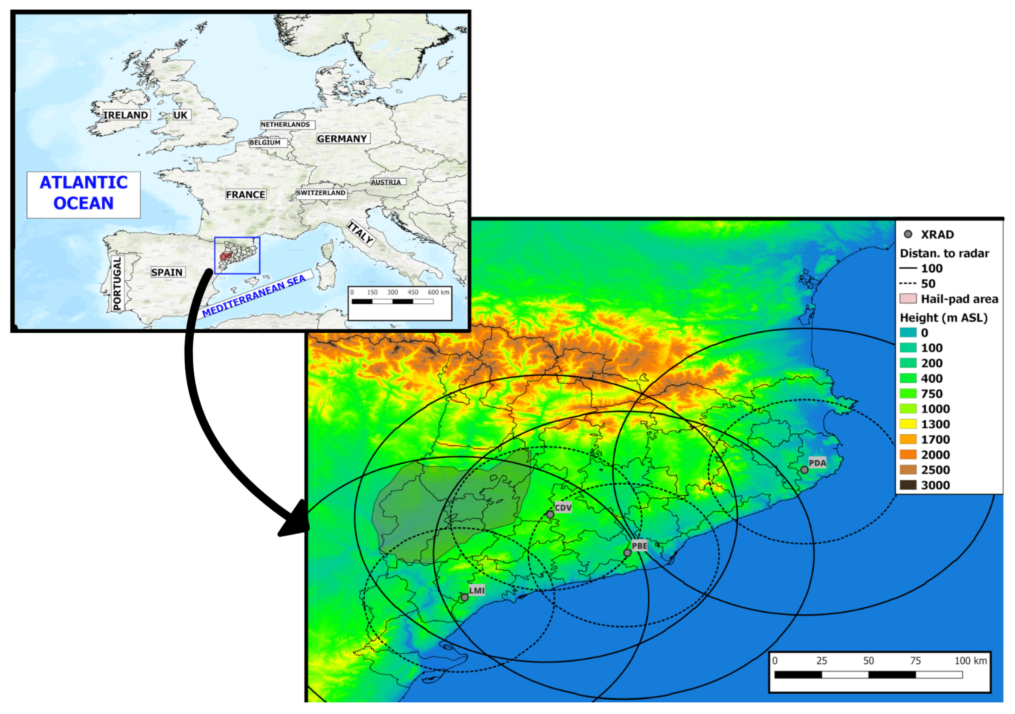
2.1. The Region of Study

As introduced previously, hailstorms hit Catalonia (NE of Iberian Peninsula, panel top-left of Figure 1) eighteen days in median, with an average of eight severe hail days, according to Rigo and Farnell [2]. The Catalan territory, with a complex topography around an area of 32,000 km², helps the development of heavy thunderstorms over the different ranges (bottom-right panel of Figure 1). The thunderstorms move to the different plains in the case of favorable atmospheric conditions, producing significant hail strikes over agricultural regions or populated areas, with corresponding damages. One of the most prone areas hit by hail events is the Western Catalan plain (bottom-right panel of Figure 1), one of the principal agricultural European regions, with a notable production of fruit trees and olives. The high interannual variability [15] of this phenomenon, the changes in the atmospheric conditions produced by global warming, the complex topography surrounding the Western Catalan plain, and the high economic impact make it necessary to adequately characterize the hail phenomenon in spatial and temporal terms.

Going more in depth in the Western Catalan plain, the region of interest is a flat area of 4241 km² with heights ranging between 70 and 600 m ASL (shaded area in the bottom-right panel of Figure 1). Different ranges surround the plain, with heights of about 800 m (East), 1000 m (South) and 1500 m (North). Meanwhile, it is open to a more extensive plain to the west. The climate is dry and cold in winter and hot in summer, with annual cumulated rainfall not exceeding 500 mm in any part of the area, according to https://www.meteo.cat/wpweb/climatologia/el-clima/atles-climatic/ (accessed on 22 August 2024). Because of this, agricultural exploitations are of two types: irrigated agriculture in those areas close to the rivers or hydraulic channels (1660 km²) and non-irrigated in the rest of the territory. Hail events occur during the year but are more likely in spring (with small size but affecting the growing season of most fruits) and summer (large hail that can destroy the fruits just before being picked).

2.2. Data Sources

The work includes two types of data sources: hail pad and radar. The following subsections describe both networks and the data type used.

2.2.1. Hail Pad Network

The ADV-Terres de Ponent manages the hail pad network of the Western Catalan plain. The SMC and the University of Leon (UL) also collaborate in the network management. Each operative location has a hail pad of 53 cm width and 31 cm length, replaced several times during each campaign for different reasons: robbery, hail hitting, wear caused by environmental conditions (mainly isolation), and damages caused by humans or animals, among others. Once a hail event hits a plaque (see an example in Figure 2), the ADV staff replaces it with a new one and provides the information to the SMC. The University of Leon reports a final analysis after a digital imagery process at the end of the campaign [19]. As Palencia et al. (2007) indicated [19], the different factors affecting the hail size measurement are the stone’s shape, the terminal velocity, the inking process, the hail dents overlapping, the software used, and the technicians’ capabilities. In particular, they found that for the six analyzed hail pads with a maximum diameter (${\mathrm{D}}_{max}$) close to 10 mm, the error ($\delta$${\mathrm{D}}_{max}$/${\mathrm{D}}_{max}$) varied between $-23$ and 0 in percentage.

In the present research, we selected the maximum size detected in each plate for 2000–2023. Because the hail research campaign in the region covers the season from April to September, we only consider the hail events that occurred during this season. The database includes registers from 211 plaques, with several registers ranging from one to 79, with an average of 37.7. These differences are because of different technical or functional causes: the staff has added some new hail pads or has removed others over the years. The registers can be with or without impacts. In this last case, the maximum stone diameter is zero. In any case, we consider them because the staff analyzed the hail pads according to the information provided by the weather radar or a spotter.

Although we have the maximum hail size registers with one decimal point precision, we characterized the ground data into only four categories:

• Null: no impacts of hail in the plaque.
• Graupel (from the Catalan word calamarsa): hail with a diameter under 0.5 cm.
• Hail: stones with a diameter between 0.5 and 2 cm.
• Severe hail: hail with a diameter over 2 cm.

This categorization minimizes the possible error caused by the calibration technique in the maximum hail diameter. However, some cases considered as hail or severe hail could probably be in the contrary group because of this error. In any case, the number of cases is negligible because only 0.55% of the sample is between 1.9 and 2.1 cm (the error range).

2.2.2. Radar Network

The XRAD (radar network of the SMC) consists of four single pol C-band radars distributed to cover volumetrically the whole territory of Catalonia (see bottom-right panel of Figure 1). Two radars (CDV and LMI in the bottom-right panel of Figure 1) fully cover the region of interest, and another one partially (PBE). This fact implies that thunderstorms that move over the Western Catalan plain are well detected and can be characterized (see panels A and B of Figure 3).

We used three types of radar data in this study: reflectivity fields (volumetric CAPPI at different levels—from 0.5 to 20 km height—with a grid size of 1 km × 1 km × 0.5 km; cross sections of the thunderstorms, to characterize them during the life cycle); daily maximum VIL fields: the maximum VIL value at each point of the grid (1 km × 1 km size) over the hail pad region, for each day with one or more ground registers (panel C of Figure 3); and daily maximum VIL density fields: the same as the VIL, but for the VIL density (panel D of Figure 3). The research compared the last two parameters with the hail pad registers.

2.3. Methodology

The structure of the research presents the following steps:

*

Identification of the potential hail days: each day with at least one register of a hail pad. The maximum hailstone diameter can be zero because each potential day the ADV staff analyzes all the possible hail pads hit by the hailstorm (because of the radar imagery or the comments of some spotters).

*

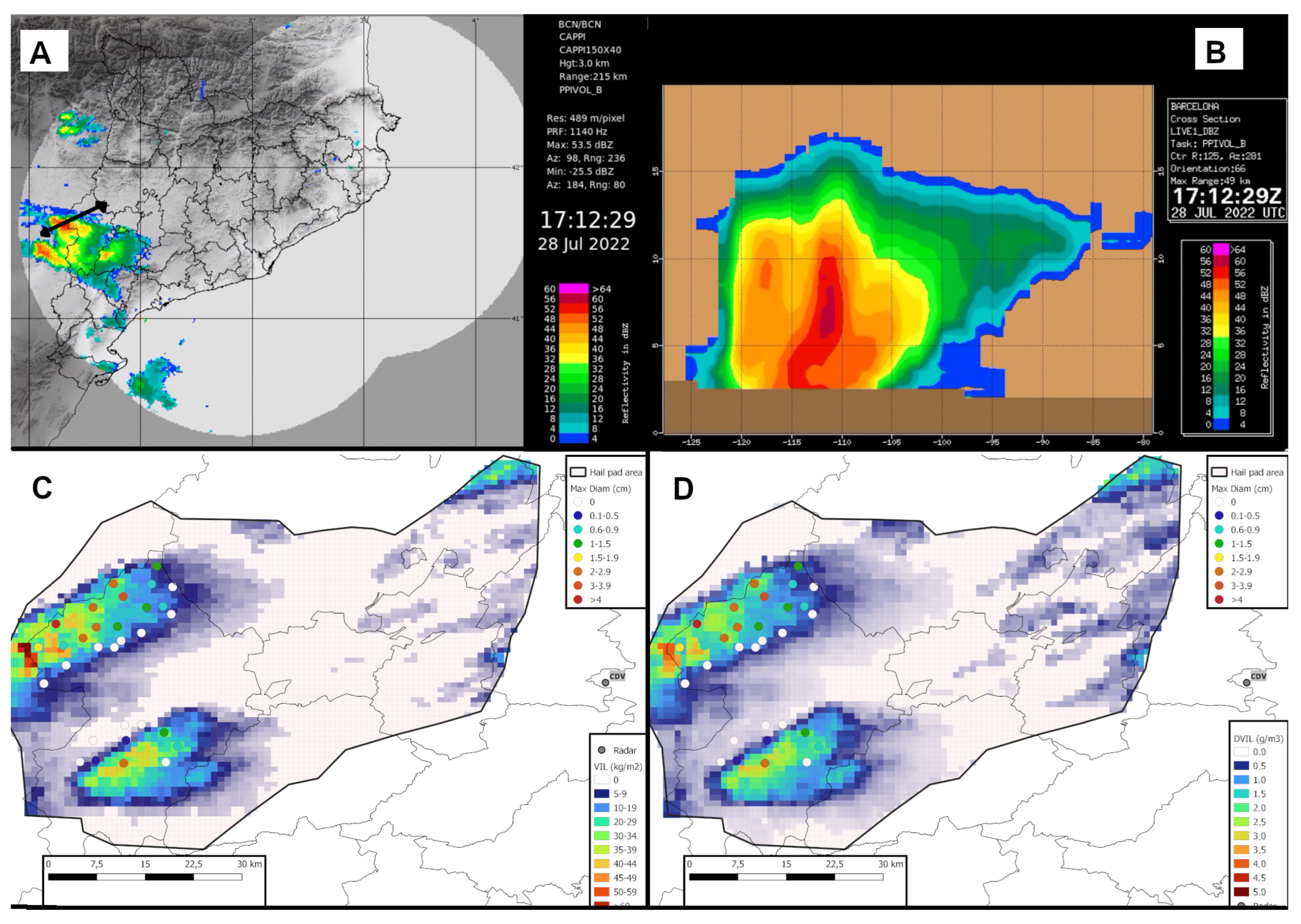
Pad characterization of the day: estimation of the centroid of the event (based on the coordinates and hail size of each of the daily registers), the maximum and mean hail size, and the area of interest (see an example in Figure 4).

*

Generation of the maximum daily VIL and VIL density fields: considering all the 6-minute instantaneous images (240 per day), we generate the maximum fields for each day of interest.

*

Radar characterization of the day: for the same region of interest in the second step, we calculate the maximum and median values of VIL and VIL density for each one of the hail pads.

Finally, each final register of the analyzed sample includes the following values:

• Date;
• The hail pad coordinates;
• The maximum hail size;
• The maximum and median VIL and VIL density.

Furthermore, each region of interest consists of an area characterized by the date, the centroid coordinates, the maximum and median hail diameter, and the maximum and median VIL and VIL density.

Figure 4. Top: each dot corresponds to an analyzed hail pad during the event of 5 July 2012. Below: normalized coordinates of the same points centered in (0, 0).

Figure 4. Top: each dot corresponds to an analyzed hail pad during the event of 5 July 2012. Below: normalized coordinates of the same points centered in (0, 0).

3. Results

3.1. Characterization of the Hail Pad Data

The hail size distribution (top panel of Figure 5) has a logarithmic shape, with an exponential decrease in the number of registers as the size increases. To verify this behavior, we fitted a linear regression to the relationship between the logarithm of the frequency and each size (considering steps of 0.5 cm), as the bottom panel of Figure 5 shows. We found that the correlation between the size and the logarithm of the frequency is $-0.907$, obtaining that the fitting equation is:

$$log\left(Freq\right)=7.995-1.439\ast size$$

(1)

The main values of this adjustment are an R-squared value of 0.8029 (indicating an acceptable correlation between the two variables), a p-value of 0.0001167 (being lower than 0.05 indicates that the sample is statistically significant), and finally, a t-value of $-6.460197$, showing there are differences between both size and frequency (logarithm) groups.

Equation (1) has only been considered in this research to show how there exists a direct relationship between the number of pads and the maximum size. However, we expect to make new comparisons considering the month of hail occurrence or by different regions to know the probability of occurrence of large hail.

Once we have observed that the hail size and the frequency are logarithmically related, we move to a time characterization of the occurrence in the region of interest. Figure 6 shows the distribution of graupel (grey), hail (blue), and severe hail (red) along the week of the year (A), the month (B), and interannually (C). The week of the year in this research starts on Monday and corresponds to one of the 52 seven-day periods that we can divide a year into. Although panels (A) and (B) show similar information, differences can be deduced that are not evident considering only one of the panels. For example, the monthly pattern shows two different behaviors, both with normal distribution (considering July as the central point): the first one, the graupel and the hail distributions present negative estimated skewness ($-0.679$ and $-0.976$, respectively) and high kurtosis values (3.135 and 4.337). Finally, the severe hail shows a positive skewness (0.259) and a small kurtosis value (1.902). These values indicate that most of the graupel and hail registers occur before July, while for the severe hail, we find most of the registers during or just after July. In addition, the graupel distribution is approximately mesokurtic (normalized shape and a mid-number of outliers). Meanwhile, hail has a leptokurtic disposal (or Laplacian pattern with few outliers), and severe hail has a platykurtic distribution (like uniform shape and many outliers).

It has not been possible to apply a normal distribution in the case of the weekly and yearly registers. However, it is worth noting that considering cumulative distribution functions allowed us to determine some trends in the three types of samples (graupel, hail, and severe hail). For the two first categories, the growth rate is constant and high during the first third of the period. After that, the rate is lower and has variations. On the other hand, the severe hail distribution starts nearly flat for the first half of the period. After this time, the increase is evident after ninety per cent of the duration when the rise stops. However, the similitude in the curves is different in the case of the yearly analysis. In this case, graupel and large hail curves are similar, while hail moves separately. The reason could be that years with more cases of hail (diameter between 0.5 and 2 cm) have fewer registers of graupel (<0.5 cm diameter) or severe hail (>2 cm).

Finally, we considered including the relationship between hail categories and the maximum daily temperature recorded in one of the automatic weather stations (AWSs) that the Servei Meteorològic the Catalunya have in the studied region (panel D in Figure 6). This graph gives an idea of the impact of the ground temperature in the different categories: graupel is more usual (82.1% of cases) in the range 22.5 to 35.0 °C and hail occurs mainly between 25 and 37.5 °C (85.9% of cases), similarly to severe hail (but with 95.8% of cases included in this temperature range). Then, the warmer the ground temperature, the higher the maximum hailstone size should be.

However, the previous behaviors change if we consider the distributions from another point of view. Figure 7 shows the same as Figure 6 but considers the percentage of registers concerning the total number of cases. This perspective considers the weight of each category each year, month, or week. For instance, the number of monthly registers for severe hail is 77 and 52 for July and September, respectively (Figure 6). However, from the new point of view, the values change to 13.4 and 14.4 (Figure 7). Then, fewer cases in September have more weight in the total distribution. With these values, the skewness changes to 0.548 (graupel), 0.403 (hail), and 0.037 (severe hail), which means that in all categories, this parameter is positive but close to neutral for the last category. In the case of the kurtosis, all the samples have values under 3, which means all have a platykurtic distribution.

3.2. Identification of the Thresholds for the Radar Variables

As has been introduced previously, the high variability of the hail in space, time, and size makes the diagnosis of the phenomenon difficult. However, the surveillance tasks need some guidelines for real time. This part of the research tries to provide some thresholds for diagnosing hail using two well-known radar products: VIL and VIL density. These products are the operational radar fields used in the Meteorological Service of Catalonia in cases of probably severe weather occurrence. Because our research purpose is to test the current operational radar products associated with hail occurring, we considered only those available in real time. We evaluated both products compared to hail pad registers. We analyzed 2816 samples by comparing the hail size estimated from the hail pad registers and the 95th percentile radar value for all the set valid points in a distance to the hail pad not larger than 3 km. In other words, we selected all the VIL or VIL density pixels surrounding the hail pad location and removed the 5% larger values to avoid outliers. A valid pixel has a value exceeding 2.5 kg/m² (for VIL) or 0.25 g/m³ (for VIL density).

The samples showed a similar distribution for all categories (no hail, graupel, hail, and severe hail) and radar parameters (VIL and VIL density). However, the distribution shape was distinct for every case, as

Table 1. Median, skewness, and kurtosis values for the distributions of VIL and VIL density (DVIL), for the null (no hail) (5137 cases), graupel (1230 pads), hail (1354 registers), and severe hail (232 cases) categories.

	VIL				DVIL
	Null	Graupel	Hail	Sev. Hail	Null	Graupel	Hail	Sev. Hail
median	0.037	0.042	0.066	0.047	0.029	0.035	0.045	0.052
skewness	1.434	0.875	0.164	1.007	1.433	1.041	0.534	0.583
kurtosis	4.363	2.297	1.386	3.243	3.881	2.456	1.618	1.507

shows. The mean, skewness, and kurtosis values are good descriptors of the distribution pattern. In the case of both radar products, the median increases as the size increases, except for severe hail, which decreases as hail size decreases. On the other hand, kurtosis and skewness decrease progressively, except, again, for severe hail and VIL (and skewness for severe hail and VIL density, but in a slight way). This anomaly for severe hail in the case of VIL is the first indicator of the worst capability of this parameter diagnosis concerning the VIL density. VIL density parameters increase (decrease) at a constant rate, indicating that this better distinguishes between the different hail categories.

The box plots shown in Figure 8 and Figure 9 provide a better understanding of the capabilities of both radar parameters to quantify the capabilities of diagnosing the hail size category. The boxes indicate the part of the sample distributed between the 25th (bottom) and the 75th (top) percentiles, while the thick line indicates the median value. The boxes show an increase with the rising size in both cases (VIL and VIL density). However, the way the increase occurs is different for both parameters. The location of the box top of the lower category (e.g., graupel) is always higher than the box bottom of the larger class (e.g., hail) in the case of VIL. Then, distinguishing between both types is difficult in certain intervals of values. This behavior is less strict in the case of the VIL density: instead of the box bottom, the limit is in the mean line, helping to discriminate the categories efficiently.

To determine the different thresholds that discriminate the four categories, we selected those values that delimitate the dominium of each category (no hail, graupel, hail, and severe hail) in Figure 10, both for VIL (top) and VIL density (below). It is necessary to consider that the used steps are 5 kg/m² for VIL and 0.5 g/m³ for VIL density. However, using lower values does not allow for better discrimination. To summarize, the selected thresholds were:

• No hail: VIL 1–12.5 kg/m², VIL density 0.1–1.25 g/m³
• Graupel: VIL 12.5–22.5 kg/m², VIL density 1.25–1.75 g/m³
• Hail: VIL 22.5–32.5 kg/m², VIL density 1.75–2.75 g/m³
• Severe hail: VIL ≥ 32.5 kg/m², VIL density ≥ 2.75 g/m³

Figure 10. VIL (top) and VIL density (bottom) distributions for all the four categories (black: no hail; grey: graupel; blue: hail; and red: severe hail).

Figure 10. VIL (top) and VIL density (bottom) distributions for all the four categories (black: no hail; grey: graupel; blue: hail; and red: severe hail).

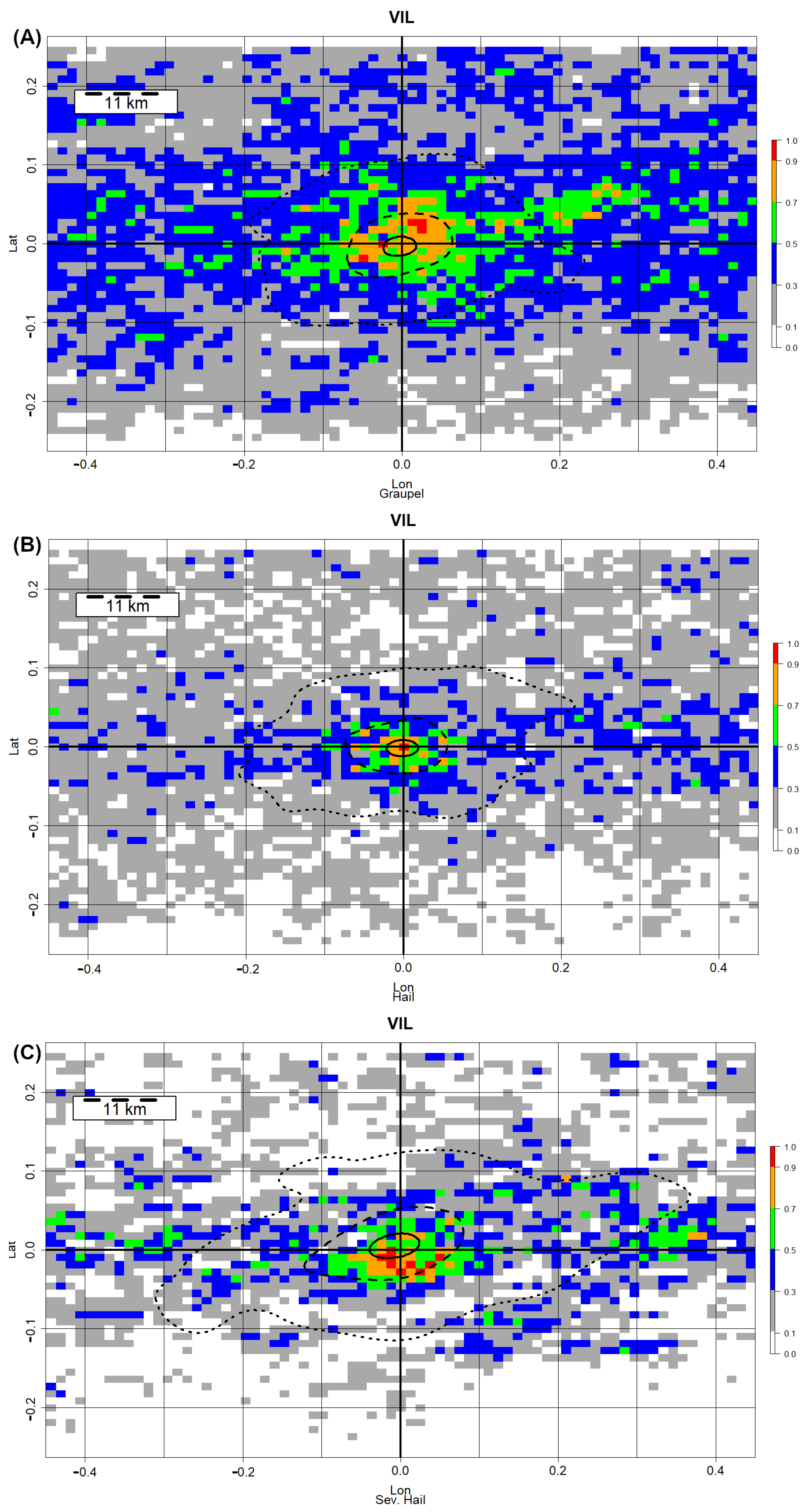
3.3. Spatial Distribution Using VIL and VIL Density: A Comparison with Ground Registers

We converted the maximum daily radar fields for both parameters (VIL and VIL density) to the maximum expected hail size according to the previous thresholds. We generated spatial distribution maps for the two products and the categories (null, graupel, hail, and severe hail) from the new fields. The purpose is to compare these distributions with the one generated through the ground registers to determine which radar product fits better to the surface occurrence. In this way, Figure 11 shows all the registers (dots) for the four categories (dark grey for null, light grey for graupel, cyan for hail, and orange for severe hail) for the period 2000–2023. The dashed lines indicate the 10th percentile of occurrence for each category (black for null, green for graupel, blue for hail, and red for severe hail), showing the usual behavior of the hailfall in the region concerning the center of the event. The shape is quite similar in all cases, with an oblate structure slightly shifted from southwest to northeast. In addition, the axes are displaced 2 km to the north and 5 km to the west. On average, all the structures have a larger axis of about 20 km and a minor axis of nearly 8 km. Finally, it is interesting to consider that the radar fields are available for 2013–2023, but the purpose is to determine if the behavior is similar.

Figure 12 shows the estimation of each hail category (graupel—panel (A), hail—panel (B), and severe hail—panel (C)) based on the maximum daily VIL fields for 2013–2023, and applying a normalization in space (centring in the middle of each area with VIL exceeding 10 kg/m²) and in the number of cases (we divide the field by the maximum value pixel), to make it comparable with the ground registers (Figure 11). Dotted, dashed, and straight lines indicate the 10th, 50th, and 90th ground observation percentiles. These lines allow comparison with the estimated radar product for the different categories, with an area overestimation of the graupel and severe hail cases, while for hail registers, the fitting looks more adjusted. Another issue occurs in the severe hail estimation: the radar field appears shifted to the south concerning the ground registers.

In the case of the VIL density (Figure 13), and using the same methodology as for VIL, the results are more adjusted to the ground truth, with a better spatial fitting for all the hail types. In the case of graupel and hail, the fit is precise for the 50th and 90th percentiles, and there is some more dispersion for the 10th percentile. The 10th and 50th percentile adjust fine in the case of severe hail, but in the case of the 90th percentile, there is a shift to the southwest, which could indicate the displacement of the larger hail registers caused by the stronger updrafts.

4. Discussion

The first issue we found at the starting point of this research is the high variability of the cases, in all senses, but we focus principally on the size, time, and space. The interannual variability found in this analysis coincides with previous works, such as [10,11,12]. In this case, there is no clear trend of the maximum hail size over the years, coinciding with other regions [15]. Furthermore, there are also coincidences in the monthly distribution with different works for the same or neighboring areas, with the maximum size during summer [16,17], or [13], or with the hail size distribution [10], with the most sample members with diameter under 2 cm.

Regarding the spatial hail distribution variability, we found only limited references focused on some specific cases [41,42]. This fact makes it difficult to compare a long-term period with event analyses. In any case, there is an agreement because the spatial distribution seems always oriented from southwest to northeast, while the largest hailstones do not usually occur over the central part of the field. This spatial distribution should be associated with two main factors: the propagation direction of hailstorms (see, for instance, the analysis of the trajectories in Rigo and Llasat (2016) [8]), which is mainly from WSW to ENE, but also with the vertical wind shear component [10], commonly perpendicular to the storm motion.

Finally, the main problem was the limited number of works that provided some significant values for discriminating operationally the hail occurrence in thunderstorms to compare with our results. In this way, probably the most accepted value is proposed by Amburn and Wolf [35] or Metzger and Nuss [43], which indicated that VIL density exceeding 3.5 g/m³ correlated well with diameters larger than 2 cm (severe hail). In the case of VIL, Edwards and Thompson [34] established 43 kg/m² as the threshold for severe hail. Stefan and Barcu [33] found that hail (of any size) occurred in Romania when VIL exceeded 55 kg/m², and VIL density was equal to or greater than 4.5 g/m³. Lastly, Ortega [44] determined that the more accurate thresholds were 25 kg/m² (any hail size) and 45 kg/m² (severe hail) for VIL and 2 g/m³ (any hail size) and 3.5 g/m³ (severe hail), for VIL density. In any case, all the analyses showed the complexity of finding thresholds that exactly fit each category. As different authors stated and Edwards and Thompson [34] briefly summarized, the radar limitations and capabilities (such as the system technologies or radar band) or the hail characteristics depending on the region or the epoch of the year make it very difficult to establish an optimal threshold valid for multiple areas and during the whole hail season. We expect that future research could include new products available in the operational chain of the Servei Meteorològic de Catalunya.

In our case, those thresholds are highly coincident, especially in the case of VIL density. Probably, the differences in the thresholds (1.75 g/m³ instead of 2 g/m³ for hail, or 2.75 g/m³ instead of 3.5 g/m³ for hail) are caused by the high precision of the hail pad measurements, with a very accurate hail size distribution [19]. In contrast, VIL threshold values are less coincident, but we also found that in our particular case, this parameter fits worst to the hail characterization. Future research should consider both the maximum hail size and the full spectrum of the hail size distribution. This second analysis results in high interest because hailstone sizes vary depending on the event. In addition, another point to develop in the early future is the influence of moisture (like temperature, shown in panel D of Figure 6) in the size of the hailstones.

5. Conclusions

The concluding remarks of this research can be summarized as follows:

• Hail time variability is similar to other regions, specially for the monthly distribution. In the case of the interannual variability, we did not find any clear trend, coinciding with other areas around the world.
• We found some thresholds for VIL and VIL density, which can be applied in real time for categorizing hail size in thunderstorms, and, on the other hand, to provide daily field maps of probable hail affectation.
• VIL density performs better than VIL in most cases.
• The comparison of radar variables and hail pad network data allows one to improve the knowledge of the spatial and time distribution of hail size.

References

1. Rigo, T.; Farnell, C. A Summary of Hail Events during the Summer of 2022 in Catalonia: A Comparison with the Period of 2013–2021. Remote Sens. 2023, 15, 1012. [Google Scholar] [CrossRef]
2. Rigo, T.; Farnell, C. The Variability of Hailfall in Catalonia and Its Climatic Implications. Climate 2023, 11, 16. [Google Scholar] [CrossRef]
3. Farnell, C.; Rigo, T.; Heymsfield, A. Shape of hail and its thermodynamic characteristics related to records in Catalonia. Atmos. Res. 2022, 271, 106098. [Google Scholar] [CrossRef]
4. Aran, M.; Pena, J.; Torà, M. Atmospheric circulation patterns associated with hail events in Lleida (Catalonia). Atmos. Res. 2011, 100, 428–438. [Google Scholar] [CrossRef]
5. Farnell, C.; Llasat, M.d.C. Proposal of three thermodynamic variables to discriminate between storms associated with hail and storms with intense rainfall in Catalonia. Tethys 2013, 10, 25–34. [Google Scholar] [CrossRef]
6. García-Ortega, E.; Fita, L.; Romero, R.; López, L.; Ramis, C.; Sánchez, J. Numerical simulation and sensitivity study of a severe hailstorm in northeast Spain. Atmos. Res. 2007, 83, 225–241. [Google Scholar] [CrossRef]
7. Rigo, T.; Farnell, C. Using maximum Vertical Integrated Liquid (VIL) maps for identifying hail-affected areas: An operative application for agricultural purposes. J. Mediterr. Meteorol. Climatol. 2019, 16, 15–24. [Google Scholar] [CrossRef]
8. Rigo, T.; Llasat, M.C. Forecasting hailfall using parameters for convective cells identified by radar. Atmos. Res. 2016, 169, 366–376. [Google Scholar] [CrossRef]
9. Farnell, C.; Rigo, T.; Pineda, N. Lightning jump as a nowcast predictor: Application to severe weather events in Catalonia. Atmos. Res. 2017, 183, 130–141. [Google Scholar] [CrossRef]
10. Marcos, J.; Sánchez, J.; Merino, A.; Melcón, P.; Mérida, G.; García-Ortega, E. Spatial and temporal variability of hail falls and estimation of maximum diameter from meteorological variables. Atmos. Res. 2021, 247, 105142. [Google Scholar] [CrossRef]
11. Barrett, B.S.; Henley, B.N. Intraseasonal variability of hail in the contiguous United States: Relationship to the Madden—Julian oscillation. Mon. Weather. Rev. 2015, 143, 1086–1103. [Google Scholar] [CrossRef]
12. Cao, Z. Severe hail frequency over Ontario, Canada: Recent trend and variability. Geophys. Res. Lett. 2008, 35. [Google Scholar] [CrossRef]
13. Hermida, L.; Sánchez, J.L.; López, L.; Berthet, C.; Dessens, J.; García-Ortega, E.; Merino, A. Climatic trends in hail precipitation in France: Spatial, altitudinal, and temporal variability. Sci. World J. 2013, 2013, 494971. [Google Scholar] [CrossRef] [PubMed]
14. Punge, H.J.; Kunz, M. Hail observations and hailstorm characteristics in Europe: A review. Atmos. Res. 2016, 176, 159–184. [Google Scholar] [CrossRef]
15. Allen, J.T.; Giammanco, I.M.; Kumjian, M.R.; Jurgen Punge, H.; Zhang, Q.; Groenemeijer, P.; Kunz, M.; Ortega, K. Understanding hail in the earth system. Rev. Geophys. 2020, 58, e2019RG000665. [Google Scholar] [CrossRef]
16. Manzato, A.; Cicogna, A.; Centore, M.; Battistutta, P.; Trevisan, M. Hailstone Characteristics in Northeast Italy from 29 Years of Hailpad Data. J. Appl. Meteorol. Climatol. 2022, 61, 1779–1795. [Google Scholar] [CrossRef]
17. Rivero-Ordaz, L.; Merino, A.; Navarro, A.; Tapiador, F.J.; Sánchez, J.L.; García-Ortega, E. Detection and characterization of hailstorms over France using DPR data onboard the GPM Core Observatory. Atmos. Res. 2024, 302, 107308. [Google Scholar] [CrossRef]
18. Malečić, B.; Cui, R.; Demory, M.E.; Horvath, K.; Jelić, D.; Schär, C.; Telišman Prtenjak, M.; Velasquez, P.; Ban, N. Simulating hail and lightning over the Alpine Adriatic region—A model intercomparison study. J. Geophys. Res. Atmos. 2023, 128, e2022JD037989. [Google Scholar] [CrossRef]
19. Palencia, C.; Berthet, C.; Massot, M.; Castro, A.; Dessens, J.; Fraile, R. On the individual calibration of hailpads. Atmos. Res. 2007, 83, 493–504. [Google Scholar] [CrossRef]
20. Lukach, M.; Foresti, L.; Giot, O.; Delobbe, L. Estimating the occurrence and severity of hail based on 10 years of observations from weather radar in B elgium. Meteorol. Appl. 2017, 24, 250–259. [Google Scholar] [CrossRef]
21. Cică, R.; Burcea, S.; Bojariu, R. Assessment of severe hailstorms and hail risk using weather radar data. Meteorol. Appl. 2015, 22, 746–753. [Google Scholar]
22. Nisi, L.; Martius, O.; Hering, A.; Kunz, M.; Germann, U. Spatial and temporal distribution of hailstorms in the Alpine region: A long-term, high resolution, radar-based analysis. Q. J. R. Meteorol. Soc. 2016, 142, 1590–1604. [Google Scholar]
23. Fluck, E.; Kunz, M.; Geissbuehler, P.; Ritz, S.P. Radar-based assessment of hail frequency in Europe. Nat. Hazards Earth Syst. Sci. 2021, 21, 683–701. [Google Scholar] [CrossRef]
24. Schuster, S.S.; Blong, R.J.; McAneney, K.J. Relationship between radar-derived hail kinetic energy and damage to insured buildings for severe hailstorms in Eastern Australia. Atmos. Res. 2006, 81, 215–235. [Google Scholar]
25. Sánchez, J.; López, L.; García-Ortega, E.; Gil, B. Nowcasting of kinetic energy of hail precipitation using radar. Atmos. Res. 2013, 123, 48–60. [Google Scholar]
26. Lindley, T.T.; Lemon, L.R. Preliminary observations of weak three-body scatter spikes associated with low-end severe hail. E-J. Sev. Storms Meteorol. 2007, 2, 1–15. [Google Scholar] [CrossRef]
27. Carbunaru, D.V.; Sasu, M.; Burcea, S.; Bell, A. Detection of hail through the three-body scattering signatures and its effects on radar algorithms observed in Romania. Atmósfera 2014, 27, 21–34. [Google Scholar]
28. Witt, A.; Nelson, S.P. The use of single-Doppler radar for estimating maximum hailstone size. J. Appl. Meteorol. Climatol. 1991, 30, 425–431. [Google Scholar] [CrossRef]
29. Blair, S.F.; Deroche, D.R.; Boustead, J.M.; Leighton, J.W.; Barjenbruch, B.L.; Gargan, W.P. A radar-based assessment of the detectability of giant hail. E-J. Sev. Storms Meteorol. 2011, 6, 1–30. [Google Scholar]
30. Kunz, M.; Kugel, P.I. Detection of hail signatures from single-polarization C-band radar reflectivity. Atmos. Res. 2015, 153, 565–577. [Google Scholar]
31. Wapler, K. The life-cycle of hailstorms: Lightning, radar reflectivity and rotation characteristics. Atmos. Res. 2017, 193, 60–72. [Google Scholar] [CrossRef]
32. Boudevillain, B.; Andrieu, H. Assessment of vertically integrated liquid (VIL) water content radar measurement. J. Atmos. Ocean. Technol. 2003, 20, 807–819. [Google Scholar] [CrossRef]
33. Stefan, S.; Barbu, N. Radar-derived parameters in hail-producing storms and the estimation of hail occurrence in Romania using a logistic regression approach. Meteorol. Appl. 2018, 25, 614–621. [Google Scholar] [CrossRef]
34. Edwards, R.; Thompson, R.L. Nationwide comparisons of hail size with WSR-88D vertically integrated liquid water and derived thermodynamic sounding data. Weather. Forecast. 1998, 13, 277–285. [Google Scholar] [CrossRef]
35. Amburn, S.A.; Wolf, P.L. VIL density as a hail indicator. Weather. Forecast. 1997, 12, 473–478. [Google Scholar] [CrossRef]
36. Farnell, C.; Rigo, T.; Martin-Vide, J. Application of cokriging techniques for the estimation of hail size. Theor. Appl. Climatol. 2018, 131, 133–151. [Google Scholar] [CrossRef]
37. Skripniková, K.; Řezáčová, D. Radar-based hail detection. Atmos. Res. 2014, 144, 175–185. [Google Scholar] [CrossRef]
38. Ochoa-Rodriguez, S.; Wang, L.P.; Willems, P.; Onof, C. A review of radar-rain gauge data merging methods and their potential for urban hydrological applications. Water Resour. Res. 2019, 55, 6356–6391. [Google Scholar] [CrossRef]
39. Kopp, J.; Manzato, A.; Hering, A.; Germann, U.; Martius, O. How observations from automatic hail sensors in Switzerland shed light on local hailfall duration and compare with hailpads measurements. Atmos. Meas. Tech. Discuss. 2023, 2023, 1–32. [Google Scholar] [CrossRef]
40. Kopp, J.; Schröer, K.; Schwierz, C.; Hering, A.; Germann, U.; Martius, O. The summer 2021 Switzerland hailstorms: Weather situation, major impacts and unique observational data. Weather 2023, 78, 184–191. [Google Scholar] [CrossRef]
41. Soderholm, J.S.; Kumjian, M.R.; McCarthy, N.; Maldonado, P.; Wang, M. Quantifying hail size distributions from the sky–application of drone aerial photogrammetry. Atmos. Meas. Tech. 2020, 13, 747–754. [Google Scholar] [CrossRef]
42. Witt, A.; Burgess, D.W.; Seimon, A.; Allen, J.T.; Snyder, J.C.; Bluestein, H.B. Rapid-scan radar observations of an Oklahoma tornadic hailstorm producing giant hail. Weather. Forecast. 2018, 33, 1263–1282. [Google Scholar] [CrossRef]
43. Metzger, E.; Nuss, W.A. The relationship between total cloud lightning behavior and radar-derived thunderstorm structure. Weather. Forecast. 2013, 28, 237–253. [Google Scholar] [CrossRef]
44. Ortega, K.L. Evaluating multi-radar, multi-sensor products for surface hailfall diagnosis. E-J. Sev. Storms Meteorol. 2018, 13, 1–36. [Google Scholar] [CrossRef]
Figure 1. Top left: Map of Western Europe. The area included in the rectangle is the region of study. Bottom right: Zoom in on the region of interest. The dots indicate the location of the radars and the circles indicate the 50 (dots) and 100 (straight) km range for each radar. The red shaded area marks the region covered by the hail pad network. “LMI”, “CDV”, “PBE”, and “PDA” indicate the locations of the radars of La Miranda, Creu del Vent, Puig Bernat, and Puig d’Arques, respectively.
Climate 12 00158 g001
Figure 2. Example of hit hail pad corresponding to the event of 29 August 2023. The image has been filtered to highlight the impacts over the plaque. The striped rectangle in the middle of the pad corresponds to the calibration area (see [19] for more information).
Climate 12 00158 g002
Figure 3. (A) CAPPI at 3 km height at 17.12 UTC on 28 July 2028. The black arrow line shows the cross section segment shown in panel (B). (B) Cross section of the thunderstorm over the region of interest at the same time as panel (A). (C) Maximum VIL field for the whole day of 28 July 2028. The dots indicate the maximum hail size registered by the different hail pads. (D) Same as panel (C), but for the maximum VIL density field.
Climate 12 00158 g003
Figure 5. Top: Hail size distribution (in logarithm) for the whole dataset of hail pad registers. Bottom: Linear fitting of the distribution.
Climate 12 00158 g005
Figure 6. From top to bottom: distribution of graupel (grey), hail (blue), and severe hail (red) for the week of the year (A), the month (B), the year (C), and the maximum daily surface temperature (D).
Climate 12 00158 g006
Figure 7. As in Figure 6, but for the percentage distribution (only for cases with plaques with impacts). (AC) panels correspond to weekly of the year, monthly, and yearly distributions, respectively.
Climate 12 00158 g007
Figure 8. Box plots of the VIL for the four hail categories detected in the hail pads (from left to right: no hail, graupel, hail and severe hail).
Climate 12 00158 g008
Figure 9. Same as Figure 8, but for VIL density.
Climate 12 00158 g009
Figure 11. Total sample of hail records (dots) for 2000–2023 (dark grey for null, grey for graupel, cyan for hail, and orange for severe hail). The dashed lines correspond to the 10th percentile of occurrence for each category (black for null, green for graupel, blue for hail, and red for severe hail), showing the usual behavior of the hailfall in the region concerning the center of the event.
Climate 12 00158 g011
Figure 12. Graupel (A), hail (B), and severe hail (C) spatial distributions estimated using maximum daily VIL fields for 2013–2023. Dotted, dashed, and straight lines indicate the 10th, 50th, and 90th ground observations percentiles.
Climate 12 00158 g012
Figure 13. Same as Figure 12, but for VIL density (Graupel, hail, and severe hail in panels (AC), respectively).
Climate 12 00158 g013