
Assessing the Value of a Human Life in Heat-Related Mortality: Lessons from COVID-19 in Belgium
VITO—Flemish Institute for Technological Research, 2400 Mol, Belgium
Climate 2024, 12(9), 129; https://doi.org/10.3390/cli12090129
Submission received: 2 August 2024
/
Revised: 21 August 2024
/
Accepted: 23 August 2024
/
Published: 26 August 2024
(This article belongs to the Special Issue Confronting the Climate Change and Health Nexus: Interactions, Impacts, and Adaptation Strategies)
Abstract
:This study evaluates the cost of heat-related mortality using economic impacts and mortality data from the COVID-19 pandemic in Belgium as a proxy. By examining the economic loss measured by gross domestic product (GDP) decline and excess mortality during the first COVID-19 wave (March–June 2020), a new estimate for avoided heat-related mortality is derived. The results show that the cost per avoided death is EUR 377,000 ± EUR 222,000, significantly lower than numerical values of the commonly used Value of a Statistical Life (VSL). However, when this cost is divided by the expected remaining (eight) life years at the age of death, the resulting monetary value for a saved life year, in a EUR 47,000 ± EUR 28,000 range, aligns well with commonly used values for the Value of a Life Year (VOLY). Thus, the present study contributes to the ongoing debate on the most appropriate methods for valuing human life in the context of heat-related mortality. By comparing our results with both VSL and VOLY, we underscore the limitations of VSL in the context of heat-related mortality and advocate for VOLY as a more accurate and contextually relevant metric. These findings may offer useful insights for policymakers in evaluating and prioritizing investments in heat-related mortality-prevention strategies.
1. Introduction
Extreme heat induces an increased incidence of premature deaths, especially in vulnerable population groups such as the elderly and persons suffering from cardiovascular disease [1]. This is a cause of concern, given that climate change projections indicate a significant rise in the frequency, duration, and intensity of extreme heat episodes. Even if the goals of the Paris Agreement to avoid dangerous climate change are achieved, a substantial rise in the frequency of deadly heat episodes is still expected [2].
In temperate climate zones, heatwaves cause more fatalities than any other weather-related disaster [3]. A notable example stems from the comparison between Hurricane Katrina in 2005, which resulted in approximately 1500 deaths [4], and the 2003 European heatwave, which led to 70,000 reported deaths [5]. Additionally, the combined death toll from the 2003 European heatwave and the 2010 Russian mega-heatwave accounted for over 80% of all deaths caused by natural disasters in Europe between 1970 and 2012 [6]. The heat-related mortality burden during the summer of 2022, the hottest season on record in Europe, has been estimated at 62,000 [7].
In July 2024, the UN Secretary General issued a call to action on extreme heat [8], underlining the urgency of the problem, among other posing severe risks to health and economic stability worldwide. The statement highlighted the need to protect those most affected by extreme heat, such as children, the urban poor, and outdoor workers; and called to boosting resilience using data and science.
City dwellers face a heightened risk of mortality from extreme heat [9,10,11]. Cities experience air temperatures in excess of rural values, especially at night, temperatures being higher by up to 7–8 °C and more. In an analysis covering Belgian cities [12], it has been found that urban areas experience twice as many heatwave days as their rural surroundings. In addition, there is evidence [13] that the urban heat island intensity itself may increase during heatwaves. While some of the increased urban mortality can be attributed to the vulnerability of urban populations, such as a higher proportion of isolated elderly individuals, it is also directly linked to the urban heat island (UHI) effect itself [14].
The mortality impact of heatwaves is often downplayed by citing the ‘harvesting’ phenomenon, where frail individuals die a few days or weeks earlier than they would have otherwise. However, this effect diminishes with stronger heatwaves. For instance, during the 2003 European heatwave, the harvesting effect was modest [15]. Overall, the number of life years remaining at death from heat-related causes has been estimated at approximately eight years [16,17].
The monetary cost of heat-related mortality is typically calculated by invoking the Value of a Statistical Life (VSL), which is an individual willingness to pay for a reduced mortality risk [18]. For example, if a survey reveals that individuals are willing to pay EUR 30 to reduce their risk of dying by one in 100,000, then the total willingness to pay would be EUR 3,000,000 (EUR 30 × 100,000). This amount represents the VSL, which in this case is EUR 3,000,000. Hence, the VSL is not the value of a specific individual’s life, but rather an aggregation of individual values for small changes in the risk of death.
From this definition, it should be clear that the VSL constitutes a highly subjective metric, being fraught with substantial uncertainty. For instance, VSL estimates across the US and Europe range from EUR 1 million to EUR 10 million [19]. Use of the VSL in the context of heat-related mortality has raised concern, considering that, often, this quantity has been established in the context of, e.g., transportation accident risks, which is very different from the mortality risks associated with heat exposure [20]. In particular, economic assessments using the Value of a Statistical Life (VSL) do not explicitly account for age, thus assuming that life expectancy at the time of death is similar across all mortality causes. However, temperature–mortality relationships indicate that heat exposure disproportionately affects older populations [11]. Some have questioned the validity of using VSL in heat-related mortality, stating that “the literature offers no heatwave-specific willingness to pay” [21], or that “the use of the VSL can be controversial” [22].
Hence, while a deeper understanding of the economic impacts of climate change on health is necessary to alert decision makers to the urgency of mitigation and to support concrete adaptation actions [21], and while the cost of heat-related mortality often dominates economic assessments of climate change impacts [23], there remains a significant level of uncertainty in determining the monetary value to be assigned to a human life.
In the present paper, we attempt to estimate the monetary cost attributed to heat-related mortality in an objective manner, by leveraging the reported economic impact of measures put in place to contain mortality during the first wave of the COVID-19 pandemic in Belgium. Concretely, the cost of avoided mortality is estimated by equating the following: (1) the welfare loss incurred during the first wave of the pandemic (March–June 2020), using gross domestic product (GDP) as a metric; (2) the estimated number of averted deaths during the same period, owing to the measures that were implemented by the government to contain the pandemic.
2. Data and Methods
2.1. COVID-19 Mortality as a Proxy for Heat-Related Mortality
Before estimating GDP loss and the associated avoided mortality, the validity of employing COVID-19 mortality as a basis for establishing heat-related mortality costs is assessed, questioning whether COVID-19 mortality serves as an adequate proxy for heat-related mortality.
The available evidence seems to indicate that it does. The health profile of people vulnerable to severe COVID-19 is very similar to that of people who are sensitive to (and die from) excessive heat [24], including the following populations:
- Elderly individuals, especially those with multiple chronic conditions and those living in nursing homes;
- People with underlying medical conditions such as cardiovascular and cerebrovascular disease, hypertension, chronic pulmonary disease, kidney disease, diabetes, obesity, Alzheimer’s disease, and dementia;
- Socially isolated persons (homeless people, migrants, older people living alone).
In addition, the expected remaining lifetime at the time of death is highly similar for heat- and COVID-19-related mortality, amounting to 7.7 years for COVID-19 [25] versus 8 years for heat-related mortality [16,17].
Considering the above elements, it is fair to say that many of the risk factors for severe COVID-19 overlap with those for heat-related mortality. Therefore, COVID-19 mortality appears to constitute a reasonable proxy for heat-related mortality.
2.2. Gross Domestic Product (GDP)
In Belgium, the first wave of the pandemic lasted from March to June 2020, leading to the largest decline in economic output since World War II. This decline was mainly related to the containment measures put in place by the government, drastically reducing the transmission of infections within the population. Starting on 14 March 2020, Belgium enforced a nationwide lockdown, closing schools, universities, restaurants, cafes, gyms, and non-essential businesses. Mobility was heavily restricted, and public gatherings were banned. These measures were gradually eased beginning 4 May 2020, allowing a phased return to social and economic activities. Note that only non-pharmaceutical measures were involved, as vaccination campaigns only began in 2021.
Gross domestic product (GDP) measures the value of all final goods and services produced within a country in a given year. Alternatively, it can be considered as the total income earned by households and businesses in a year [26]. A decline in GDP indicates a reduction in economic activity and is associated with job losses, reduced working hours, lower wages, and overall lower income levels for businesses and individuals. All these factors constitute a direct cost to the community.
In Belgium, quarterly GDP is published by the National Bank of Belgium [27]. Their estimates are based on national and regional accounts, which are compiled according to the requirements of the European System of Accounts (ESA 2010) [28], which is an internationally compatible EU accounting framework for a systematic and detailed description of an economy.
Table 1 presents reported GDP values for quarters 1 and 2, as well as their sum, for recent years. The consideration of only the first two quarters relates to the fact that the paper focuses on the first COVID-19 wave, which occurred between March and June 2020, i.e., within quarters 1 and 2 of that year.
2.3. COVID-19 Mortality
In early March 2020, the Belgian health institute Sciensano was mandated by the regional and federal authorities with the task to gather daily nationwide COVID-19 mortality figures [29]. Considering that the standard registration procedure of the specific causes of death is a rather slow process, an ad hoc surveillance was established to allow the near-real-time monitoring of COVID-19 mortality. A centralized data registration was established, gathering data from hospitals, long-term health care facilities, and general practitioners.
Death reporting was exhaustive, including all deaths potentially attributable to the pandemic, irrespective of the diagnostic method and setting. Subsequent studies showed that the ratio between observed overall excess mortality and reported COVID-19 mortality was remarkably close to unity in Belgium [30,31,32,33]. This consistent reporting of comprehensive and reliable mortality figures makes the Belgian data particularly suitable for use in quantitative studies as the one presented here.
2.4. Epidemiological Modelling
One of the main challenges of the approach presented here is the estimation of the hypothetical number of avoided deaths that would have occurred in the absence of any containment measures. Apart from adopting insights from the literature, we will apply an epidemiological model to evaluate scenarios of pandemic containment, in particular scenarios based on measures taken by individuals at a modest or no economic cost, as opposed to the nationwide lockdown imposed by the government.
The epidemiological model used here to simulate the evolution of the pandemic and to assess the potential number of averted deaths is the compartmental model developed by De Visscher [35]. This model simulates the time evolution of the number of uninfected (), infected (), sick (), very sick (), better (), recovered (), and deceased () individuals. In the remainder of this paper the ‘better’ and ‘recovered’ categories will be disregarded as our focus is on mortality only and considering that the omission of these categories has no bearing on mortality outcomes.
The model is based on the following system of coupled ordinary differential equations (an overhead dot denoting a time derivative):
In these equations, the total population () is set at 11.5 million, the total Belgian population in early 2020. The symbols shown between brackets refer to the transfer rates between compartments, as graphically shown in Figure 2. The coefficients are fixed to values that represent COVID-19 characteristics [35], such as the incubation time. The coefficient holds a central position, being related to the reproduction number (see above) through , with (the units of being days−1). Unlike the other coefficients, it is an adjustable parameter in the model.
The model contains a mechanism to simulate the impact of measures aiming to reduce by introducing an effectiveness with the subscripts refer to the reproduction number before and after the introduction of a measure, such as a lockdown. A measure that is 100% effective () would bring to zero, effectively terminating the spread of the virus. A measure with an effectiveness of 0% corresponds to a situation without any mitigating measures at all.
The system of ordinary differential Equations (1)−(5) is solved using Runge–Kutta–Fehlberg (RKF45) integration over the period from 1 February to 30 June 2020. The coefficients and were adjusted until the model yielded a satisfactory match with daily number of deaths observed in Belgium (Figure 1), resulting in and . The value obtained for the reproduction number matches nicely with independent estimates of [36]. The infection fatality rate (IFR), having a default value in the model of 1.5%, was kept as this value coincides well with reported values for Belgium of 1.47% [32] and 1.251−1.672% [37].
With these parameter values, the modelled cumulative number of deaths matches the reported number within 0.5% (Figure 1). The time tendencies simulated for the various model compartments using these calibrated parameters are shown for Belgium for February−June 2020 in Figure 3.
The conclusion of this subsection is that the model is capable of correctly reproducing daily and accumulated deaths in the period February−June 2020, including the effect of the lockdown (through the parameter ). More details regarding the model and its applications are available in the paper by De Visscher [35].
3. Results
3.1. Net Loss of Gross Domestic Product (GDP)
The economic cost resulting from the containment measures is assessed by examining the net GDP decrease occurring during quarters 1 and 2 of 2020 (i.e., covering the first COVID-19 wave) in comparison to what would have occurred in a hypothetical non-COVID-19 scenario.
According to data from the National Bank of Belgium (Table 1), in the years leading up to 2020, the GDP value of the combined first and second quarters consistently rose by approximately EUR 7.3 billion compared to the same period of the previous year. Extrapolating this tendency (Figure 4) through linear regression yields, we obtain a predicted GDP value for the first two quarters of the year 2020 (in the absence of COVID-19) of EUR 241.4 billion ± EUR 2.7 billion (95% confidence interval).
Conversely, during the first half of 2020, the reported actual GDP reached a value of only EUR 222.0 billion, implying a net decrease of EUR 19.4 billion ± EUR 2.7 billion during the first wave of COVID-19 in Belgium in comparison to the hypothetical situation in which no pandemic had arisen.
3.2. Number of Lives Saved Due to the Lockdown
The number of lives saved due to the lockdown was estimated by comparing the number of actual deaths (approximately 10,000, see above) with the number of deaths that would have occurred in the absence of the lockdown.
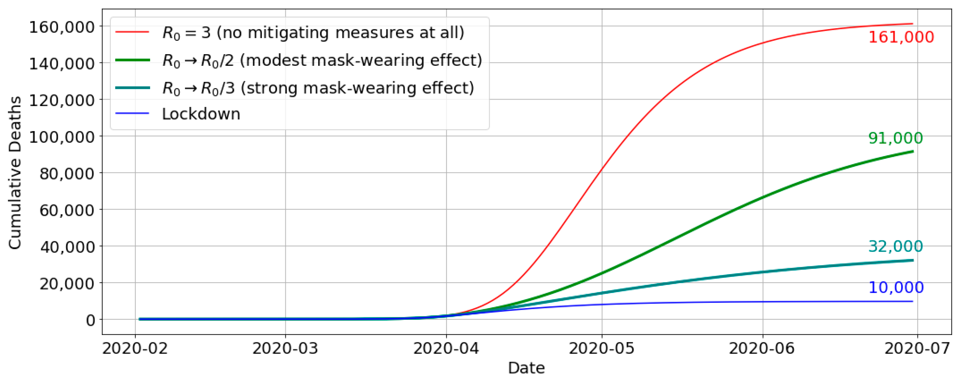
The latter was assessed by means of the compartmental model described in Section 2.4, setting the efficiency of the imposed measures at 0% (), thus removing any mitigating measures. Figure 5 shows that, over the concerned period February−June 2020, this would have led to 161,000 deaths, or approximately 151,000 extra deaths compared to the actual reported number.
Other studies have reached similar numbers. For instance, a study on European COVID-19 mortality [38] found that, for Belgium, the absence of mitigating measures would have led to 120,000 deaths by May 4. (The model of Section 2.4 used in the present analysis is a bit more conservative, predicting 93,000 deaths for that date.)
Yet, these high estimates do not account for individual changes in behaviour. They ignore the fact that, in the presence of a raging pandemic, people would have applied self-imposed measures, thus reducing the reproduction number [38]. Several studies ascertain that such measures, such as wearing a mask or working remotely, have an effect of the same magnitude as the official, population-level, public health intervention measures [39,40].
Masks are the most cost-effective of non-pharmaceutical interventions, having relatively few adverse effects on the economy [41]. Analysis has shown the strong potential effect of mask wearing on reducing the reproduction number, with reductions by a factor in the range of 2−3 for plausible ranges of public uptake (75−90%) and mask effectiveness (0.5−0.7) [42]. When implementing this range of , reductions in the model described above (Section 2.4), the number of deaths is reduced from 161,000 (no mitigation) to 91,000 ( reduced by a factor of 2) resp. 33,000 ( reduced by a factor of 2) (Figure 5).
This means that, in the absence of any government interventions, a simple and cost-effective measure such as self-imposed mask-wearing would have resulted in a number of deaths between 33,000 and 91,000, or 62,000 ± 29,000. In other words, compared to the 10,000 deaths that effectively occurred during this period, 52,000 ± 29,000 deaths may have been avoided due to the measures imposed by the government. The large uncertainty in this estimate reflects the hypothetical nature of estimating the potentially avoided (counterfactual) number of deaths. Nevertheless, our estimate is consistent with an independent assessment [43], suggesting that 50,000 deaths were avoided due to the lockdown during the first COVID-19 wave in Belgium.
3.3. Cost per Avoided Death
In the previous subsections, the following findings were presented:
- The net GDP loss caused by the lockdown amounts to EUR 19.4 billion ± EUR 2.7 billion;
- The number of avoided deaths due to the lockdown is estimated at 52,000 ± 29,000.
Putting these two results together, the cost per avoided death is obtained by dividing the net GDP loss by the number of avoided deaths. Incorporating error propagation, a value of EUR 377,000 ± EUR 222,000 is obtained as the cost per prevented fatality, i.e., the value that has implicitly been assigned to a human life through the containment measures.
4. Discussion
The monetary value assigned to a human life in this study, estimated at EUR 377,000 ± EUR 222,000, stands in stark contrast to the Value of a Statistical Life (VSL) typically cited in the literature, which ranges between EUR 1 million and EUR 10 million [19] (see the Introduction Section).
This discrepancy is not unexpected given the fundamentally different constructs these values represent. While the VSL is derived from willingness-to-pay (WTP) studies that assess how much individuals are willing to pay to reduce their risk of dying, our estimate is based on actual economic losses incurred during the COVID-19 pandemic. The VSL method aggregates individual preferences across small changes in mortality risk, often in contexts like transportation accidents, which involve different demographic profiles and risk perceptions than those associated with heat-related mortality [22,44].
Moreover, the VSL does not explicitly account for age, instead assuming a uniform life expectancy across all causes of death. However, empirical evidence consistently shows that heat exposure disproportionately affects older populations, who have fewer remaining life years at the time of death [11]. This assumption introduces a significant bias when applying VSL to heat-related mortality, where the affected demographic group primarily consists of the elderly. As such, using VSL in this context can lead to overestimation of the economic value of avoided deaths.
Our study’s estimate aligns more closely with the Value of a Life Year (VOLY), which is designed to account for the remaining life expectancy at the time of death. When we divide our estimate of EUR 377,000 ± EUR 222,000 by the average remaining life years (approximately eight years for heat-related deaths), the resulting VOLY of EUR 47,000 ± EUR 28,000 falls within the range recommended for European countries (EUR 25,000–EUR 100,000) [44]. This suggests that VOLY may be a more appropriate metric for valuing lives in the context of climate-related mortality, particularly for older populations.
Furthermore, the significant disparity between VSL and VOLY observed here echoes findings in the broader literature, where differences of up to an order of magnitude have been reported [45,46]. Such disparities underscore the inherent uncertainties in these metrics and the importance of context-specific valuation methods. One study noted that relying on VSL can lead to substantially higher estimates compared to VOLY, especially when applied to scenarios involving predominantly older individuals [17], concluding that “this is a major and far from resolved source of uncertainty in economic terms”. Our analysis, therefore, suggests that VOLY should be the preferred approach for economic evaluations of heat-related mortality, given its closer alignment with the actual demographic characteristics of the affected population.
It is insightful to apply the monetary value assigned to human life to estimates of projected future heat-related mortality. Currently, average heat-related mortality in Belgium stands at approximately 70 excess deaths per year (reference period 1980–2010). Future projections estimate that the annual average of heat-related deaths could increase to around 2800 by the end of the century under a high climate scenario (2837 annual deaths under RCP8.5 are cited in [23] and 2777 annual deaths under SSP5-8.5 in [47]). Multiplying this projected figure of 2800 annual deaths by the previously calculated value of human life results in an estimated economic burden of approximately EUR 1 billion per year, though this figure comes with a substantial uncertainty range (EUR 0.43 billion to EUR 1.67 billion).
Applying this methodology to other types of mortality, such as that associated with respiratory infections, cardiac arrest, or lung cancer, appears feasible as long as the VOLY figure (EUR 43,000) is used. The primary challenge lies in accurately estimating the expected remaining life years at the age of death, which may vary significantly across different ailments compared to the eight years assumed for COVID-19 and heat-related mortality.
5. Conclusions
In this paper, we made an attempt to assess the cost of heat-related mortality by using COVID-19 mortality as a proxy. Our approach focused on Belgium during the first COVID-19 wave (March–June 2020), since this period was exceptionally well documented, and highly accurate daily mortality figures were available. The underlying idea is that the economic losses caused by to the lockdown can be equated to the numerous lives saved due to the lockdown, leading to a unit cost per life saved.
First, it was argued that COVID-19 mortality is indeed a suitable proxy for heat-related mortality. Not only are vulnerable population groups for both COVID-19 and heat nearly identical (elderly people and people with pre-existing disease), the potential number of life years remaining at the age of death is also very similar, being approximately eight years for either.
The monetary cost that can be assigned to a human life under COVID-19 (and by extension, to heat-related mortality) was established by linking the following factors:
- The net loss in the gross domestic product (GDP) occurring in the first half of the year 2020 (i.e., the period encompassing the first COVID-19 wave) due to the measures taken by the government, which was estimated to represent a loss of 19.4 billion ± EUR 2.7 billion;
- The number of avoided deaths due to the lockdown, estimated using evidence from the literature and through epidemiological modelling, considering the hypothetical number of people that were saved due to the measures taken by the government, their number amounting to 52,000 ± 29,000.
The resulting monetary cost of avoiding one death was found to be EUR 377,000 ± EUR 222,000. This amount turns out to be an order of magnitude lower than commonly used values for the Value of a Statistical Life (VSL). Among other things, this was attributed to the relatively short stretch of expected life years remaining at the age of death for extreme heat as compared to all causes of death. As a consequence, when reducing our estimate for the monetary cost of a human life to an annual cost, by dividing by the presumed eight life years remaining at the age of death, the resulting range of EUR 19,000–EUR 75,000 is much closer to the generally accepted values for the Value of a Life Year (VOLY).
The novelty of the approach presented here is that, rather than assessing the cost of a human life based on an individual willingness to pay, it is assessed as an actual collective willingness to pay. This may even be the more appropriate way to go, considering that the cost of climate action and adaptive interventions is borne by collectivity. The main new insight is that our analysis identifies the VOLY, together with a life expectance at the age of death of 8 years, as the preferred approach for quantifying heat-related mortality cost. As mentioned in the Introduction Section, quite some uncertainty regarding the VSL vs. VOLY approach has existed so far; our findings clearly identify the latter as the most appropriate metric.
The relevance and application of these results lie in their utility for supporting cost–benefit assessments of heat-related health climate actions. Mortality cost figures provide critical evidence for decision making, bolstering the case for investments in health protection and serving as a baseline against which the effectiveness of protective measures can be monitored [48]. The significance of these protective measures cannot be overstated. For instance, it has been demonstrated that the heat-related health action plans implemented after the deadly 2003 heatwave in France resulted in a nearly 70% reduction in mortality during the extreme heatwave of 2006 [49]. More recently, an analysis of heat-related mortality in Europe concluded that the death toll during the summer of 2023, which reached nearly 50,000, would have been 80% higher without adaptive actions [50]. Many of these adaptive actions focus on early warning and behavioural changes, which have been found to be highly cost effective; in fact, estimates for France show that the annual operating costs for a heat-related health action plan involves an annual operating cost of EUR 455,000 [21], which is at the same level of cost as that estimated here for a single human life.
This shows that there is ample room to consider additional measures, in particular those targeting infrastructure and urban planning. Urban interventions are not only relevant because of the elevated temperatures occurring in cities, such interventions may also be more efficient considering the high density of people that may benefit from them [51]. One measure that is considered particularly useful in an urban context consists of increasing the abundance of green urban infrastructure [47,52,53]. A study involving 100 European cities [54] has shown that a large potential for additional cooling by greening remains in many cities. While such infrastructural and planning measures are more costly than, e.g., behavioural changes, they bring benefits that last for years or decades. Moreover, urban greening measures bring many other benefits, including a positive impact on the physical and mental health of urban dwellers.
Our analysis has several limitations. First, the number of averted fatalities only accounts for mortality directly associated with COVID-19 infections. It does not account for mortality that might otherwise have been affected by the pandemic, owing to the reduced health care for non-COVID-19 disease, including cancers going undetected and urgent care being postponed [31]. At the same time, the lockdowns have also led to a reduction in certain types of fatalities, such as those related to traffic accidents. Still, balancing all these effects is far from straightforward, which is why they were left out.
Moreover, our approach is limited with respect to the monetary metric used, i.e., net GDP loss, which was used to estimate the amount of wealth a country is prepared to forego to save people from dying. Indeed, other ways to quantify the willingness to pay for a human life (or life year) are available. For instance, the WHO considers a cost per QALY (Quality Adjusted Life Year) of one–three times the GDP per capita as cost-effective [55]. Interestingly, with a Belgian GDP per capita of EUR 43,000 (2019 value), we arrive at a range of EUR 43,000–EUR 129,000 per QALY, suggesting slightly lower values for the VOLY, i.e., not significantly different from our VOLY estimate of EUR 19,000–EUR 75,000.
Finally, the results obtained here cannot easily be transposed to other regions, especially low- or middle-income countries, considering that any pandemic containment measures would probably induce GDP shocks of a different intensity. Also, such countries generally feature a different population age distribution, with a lower share of elderly people, which would affect epidemiological aspects such as the infection fatality rate (IFR). Still, with suitable data regarding actual mortality and net GDP loss, the methodology described in this paper could be replicated to other regions, which will be the subject of future research.
Funding
This research received no external funding.
Data Availability Statement
Belgian COVID-19 mortality data are available from the ‘Belgium COVID-19 Dashboard, Sciensano’ Belgium COVID-19 Epidemiological Situation—Deaths. Available online: https://lookerstudio.google.com/embed/reporting/c14a5cfc-cab7-4812-848c-0369173148ab/page/QTSKB (accessed on 1 August 2024). (Right-Click on the Graph ‘Daily New Deaths’ and Select ‘Export’ to Download a Csv File Containing the Data). Belgian quarterly gross domestic product (GDP) data are available from the National Bank of Belgium. National Accounts—Quarterly and Annual Aggregates. 2023. Available online: https://stat.nbb.be/ (accessed on 27 June 2024). (On the left-hand menu, select ‘National accounts’, then ‘Quarterly and annual aggregates’, again select ‘Quarterly and annual aggregates’, then ‘Gross value added by branch of activity’; adjust the ‘Time’ range and consider the ‘Total economy’ figures.)
Conflicts of Interest
Author Koen De Ridder was employed by the company VITO—Flemish Institute for Technological Research. The author declare that the research was conducted in the absence of any commercial or financial relationships that could be construed as a potential conflict of interest.
References
- van Daalen, K.R.; Tonne, C.; Semenza, J.C.; Rocklöv, J.; Markandya, A.; Dasandi, N.; Jankin, S.; Achebak, H.; Ballester, J.; Bechara, H.; et al. The 2024 Europe report of the Lancet Countdown on health and climate change: Unprecedented warming demands unprecedented action. Lancet Public Health 2024, 9, e495–e522. [Google Scholar] [CrossRef] [PubMed]
- Matthews, T.K.R.; Wilby, R.L.; Murphy, C. Communicating the deadly consequences of global warming for human heat stress. Proc. Natl. Acad. Sci. USA 2017, 114, 3861–3866. [Google Scholar] [CrossRef]
- Borden, K.A.; Cutter, S.L. Spatial patterns of natural hazards mortality in the United States. Int. J. Health Geograph. 2008, 7, 64. [Google Scholar] [CrossRef] [PubMed]
- Beven, J.L., II; Avila, L.A.; Blake, E.S.; Brown, D.P.; Franklin, J.L.; Knabb, R.D.; Pasch, R.J.; Rhome, J.R.; Stewart, S.R. Atlantic Hurricane Season of 2005. Mon. Weather Rev. 2008, 136, 1109–1173. [Google Scholar] [CrossRef]
- Robine, J.-M.; Cheung, S.L.K.; le Roy, S.; van Oyen, H.; Griffiths, C.; Michel, J.-P.; Herrmann, F.R. Death toll exceeded 70,000 in Europe during the summer of 2003. Comptes. Rendus. Biol. 2008, 331, 171–178. [Google Scholar] [CrossRef]
- Golnaraghi, M.; Etienne, C.; Guha-Sapir, D.; Below, R. Atlas of Mortality and Economic Losses from Weather, Climate and Water Extremes (1970–2012); World Meteorological Organization: Geneva, Switzerland, 2014; ISBN 978-92-63-11123-4. Available online: https://library.wmo.int/idurl/4/57564 (accessed on 22 August 2024).
- Ballester, J.; Quijal-Zamorano, M.; Méndez Turrubiates, R.F.; Pegenaute, F.; Herrmann, F.R.; Robine, J.M.; Basagaña, X.; Tonne, C.; Antó, J.M.; Achebak, H. Heat-related mortality in Europe during the summer of 2022. Nat. Med. 2023, 29, 1857–1866. [Google Scholar] [CrossRef] [PubMed]
- United Nations Secretary-General’s Call to Action on Extreme Heat. 25 July 2024. Available online: https://www.un.org/sites/un2.un.org/files/unsg_call_to_action_on_extreme_heat_for_release.pdf (accessed on 2 August 2024).
- Gabriel, K.M.A.; Endlicher, W.R. Urban and rural mortality rates during heatwaves in Berlin and Brandenburg, Germany. Environ. Poll. 2011, 159, 2044–2050. [Google Scholar] [CrossRef] [PubMed]
- Dousset, B.; Gourmelon, F.; Laaidi, K.; Zeghnoun, A.; Giraudet, E.; Bretin, P.; Maurid, E.; Vandentorren, S. Satellite monitoring of summer heatwaves in the Paris metropolitan area. Int. J. Climatol. 2011, 31, 313–323. [Google Scholar] [CrossRef]
- Huang, W.T.K.; Masselot, P.; Bou-Zeid, E.; Fatichi, S.; Paschalis, A.; Sun, T.; Gasparrini, A.; Manoli, G. Economic valuation of temperature-related mortality attributed to urban heat islands in European cities. Nat. Commun. 2023, 14, 7438. [Google Scholar] [CrossRef]
- Wouters, H.; De Ridder, K.; Poelmans, L.; Willems, P.; Brouwers, J.; Hosseinzadehtalaei, P.; Tabari, H.; Vanden Broucke, S.; van Lipzig, N.P.M.; Demuzere, M. Heat stress increase under climate change twice as large in cities as in rural areas: A study for a densely populated midlatitude maritime region. Geophys. Res. Lett. 2017, 44, 8997–9007. [Google Scholar] [CrossRef]
- De Ridder, K.; Maiheu, B.; Lauwaet, D.; Daglis, I.A.; Keramitsoglou, I.; Kourtidis, K.; Manunta, P.; Paganini, M. Urban Heat Island Intensification during Hot Spells—The Case of Paris during the Summer of 2003. Urban Sci. 2017, 1, 3. [Google Scholar] [CrossRef]
- Keller, R.C. Fatal Isolation: The Devastating Paris Heatwave of 2003; University of Chicago Press: Chicago, IL, USA, 2015; 240p. [Google Scholar]
- Toulemon, L.; Barbieri, M. The mortality impact of the August 2003 heatwave in France: Investigating the ‘harvesting’ effect and other long-term consequences. Popul. Stud. 2008, 62, 39–53. [Google Scholar] [CrossRef]
- Bosello, F.; Schechter, M. Integrated socio-economic assessment. In Regional Assessment of Climate Change in the Medi-Terranean. Vol. 2: Agriculture, Forests, Ecosystem Services and People; Navarra, A., Tubiana, L., Eds.; Springer: Berlin/Heidelberg, Germany, 2013; 402p. [Google Scholar]
- Sánchez-Martínez, G.; Williams, E.; Yu, S.S. The economics of health damage and adaptation to climate change in Europe: A review of the conventional and grey literature. Climate 2015, 3, 522–541. [Google Scholar] [CrossRef]
- OECD. Mortality Risk Valuation in Environment, Health and Transport Policies; OECD Publishing: Paris, France, 2012. [Google Scholar] [CrossRef]
- Ciscar, J.C.; Rising, J.; Kopp, R.E.; Feyen, L. Assessing future climate change impacts in the EU and the USA: Insights and lessons from two continental-scale projects. Environ. Res. Lett. 2019, 14, 084010. [Google Scholar] [CrossRef]
- Ščasný, M.; Alberini, A. Valuation of Mortality Risk Attributable to Climate Change: Investigating the Effect of Survey Administration Modes on a VSL. Int. J. Environ. Res. Public Health 2012, 9, 4760–4781. [Google Scholar] [CrossRef] [PubMed]
- Adélaïde, L.; Chanel, O.; Pascal, M. Health effects from heat waves in France: An economic evaluation. Eur. J. Health Econ. 2022, 23, 119–131. [Google Scholar] [CrossRef] [PubMed]
- Szewczyk, W.; Feyen, L.; Matei, A.; Ciscar, J.C.; Mulholland, E.; Soria, A. Economic Analysis of Selected Climate Impacts; EUR 30199 EN; Publications Office of the European Union: Luxembourg, 2020; Available online: https://data.europa.eu/doi/10.2760/845605 (accessed on 22 August 2024).
- Forzieri, G.; Cescatti, A.; Batista e Silva, F.; Feyen, L. Increasing risk over time of weather-related hazards to the European population: A data-driven prognostic study. Lancet Planet. Health 2017, 1, e200–e208. [Google Scholar] [CrossRef]
- World Health Organization. Care for Vulnerable Population Groups: Updated Evidence on Risk Factors and Vulnerability in Heat and Health in the WHO European Region: Updated Evidence for Effective Prevention; Sánchez-Martínez, G., de’Donato, F., Kendrovski, V., Eds.; World Health Organization: Copenhagen, Denmark, 2021; pp. 97–120. Available online: https://iris.who.int/bitstream/handle/10665/339462/9789289055406-eng.pdf (accessed on 22 August 2024).
- Vandresse, M. Belgium—Excess Mortality in 2020: 124,000 Years of Life Lost (Federal Planning Bureau Fact Sheet No. 5). 2021. Available online: https://www.plan.be/uploaded/documents/202105100808300.FACTSHEET_005_DEMO_12407_E.pdf (accessed on 27 June 2024).
- Shapiro, D.; MacDonald, D.; Greenlaw, S.A. Principles of Economics, 3rd ed.; OpenStax Rice University, 2022; Available online: https://openstax.org/details/books/principles-economics-3e (accessed on 22 August 2024).
- National Bank of Belgium. National Accounts—Quarterly and Annual Aggregates. 2023. Available online: https://stat.nbb.be/ (accessed on 27 June 2024).
- European Union. European System of Accounts (ESA 2010). Eurostat, Manual and Guidelines. 2013. Available online: https://doi.org/10.2785/16644 (accessed on 30 July 2024).
- Renard, F.; Scohy, A.; Van der Heyden, J.; Peeters, I.; Dequeker, S.; Vandael, E.; Van Goethem, N.; Dubourg, D.; De Viron, L.; Kongs, A.; et al. Establishing an ad hoc COVID-19 mortality surveillance during the first epidemic wave in Belgium, 1 March to 21 June 2020. Eurosurveillance 2021, 26, 2001402. [Google Scholar] [CrossRef]
- Bustos Sierra, N.; Bossuyt, N.; Braeye, T.; Leroy, M.; Moyersoen, I.; Peeters, I.; Scohy, A.; Van der Heyden, J.; Van Oyen, H. All-cause mortality supports the COVID-19 mortality in Belgium and comparison with major fatal events of the last century. Arch. Public Health 2020, 78, 117. [Google Scholar] [CrossRef]
- Luyten, J.; Schokkaert, E. Belgium’s response to the COVID-19 pandemic. Health Econ. Policy Law 2021, 17, 37–47. [Google Scholar] [CrossRef]
- Molenberghs, G.; Faes, C.; Verbeeck, J.; Deboosere, P.; Abrams, S.; Willem, L.; Aerts, J.; Theeten, H.; Devleesschauwer, B.; Bustos Sierra, N.; et al. COVID-19 mortality, excess mortality, deaths per million and infection fatality ratio, Belgium, 9 March 2020 to 28 June 2020. Eurosurveillance 2022, 27, 2002060. [Google Scholar] [CrossRef] [PubMed]
- COVID-19 Excess Mortality Collaborators. Estimating excess mortality due to the COVID-19 pandemic: A systematic analysis of COVID-19-related mortality, 2020–2021. Lancet 2022, 399, 1513–1536. [Google Scholar] [CrossRef]
- Belgium COVID-19 Epidemiological Situation—Deaths. Belgium COVID-19 Dashboard, Sciensano. (Right-Click on the Graph ‘Daily New Deaths’ and Select ‘Export’ to Download a Csv File Containing the Data). Available online: https://lookerstudio.google.com/embed/reporting/c14a5cfc-cab7-4812-848c-0369173148ab/page/QTSKB (accessed on 1 August 2024).
- De Visscher, A. The COVID-19 pandemic: Model-based evaluation of non-pharmaceutical interventions and prognoses. Nonlinear Dyn. 2020, 101, 1871–1887. [Google Scholar] [CrossRef]
- Abrams, S.; Wambua, J.; Santermans, E.; Willem, L.; Kuylen, E.; Coletti, P.; Libin, P.; Faes, C.; Petrof, O.; Herzog, S.A.; et al. Modelling the early phase of the Belgian COVID-19 epidemic using a stochastic compartmental model and studying its implied future trajectories. Epidemics 2021, 35, 100449. [Google Scholar] [CrossRef]
- COVID-19 Forecasting Team. Variation in the COVID-19 infection-fatality ratio by age, time, and geography during the pre-vaccine era: A systematic analysis. Lancet 2022, 399, 1469–1488. [Google Scholar] [CrossRef] [PubMed]
- Flaxman, S.; Mishra, S.; Gandy, A.; Unwin, H.J.T.; Mellan, T.A.; Coupland, H.; Whittaker, C.; Zhu, H.; Berah, T.; Eaton, J.W.; et al. Estimating the effects of non-pharmaceutical interventions on COVID-19 in Europe. Nature 2020, 584, 257–261. [Google Scholar] [CrossRef]
- Jamison, J.C.; Bundy, D.; Jamison, D.T.; Spitz, J.; Verguet, S. Comparing the impact on COVID-19 mortality of self-imposed behavior change and of government regulations across 13 countries. Health Serv. Res. 2021, 56, 874–884. [Google Scholar] [CrossRef]
- Lison, A.; Banholzer, N.; Sharma, M.; Mindermann, S.; Unwin, H.J.T.; Mishra, S.; Stadler, T.; Bhatt, S.; Ferguson, N.M.; Brauner, J.; et al. Effectiveness assessment of non-pharmaceutical interventions: Lessons learned from the COVID-19 pandemic. Lancet Public Health 2023, 8, e311–e317. [Google Scholar] [CrossRef]
- Agyapon-Ntra, K.; McSharry, P.E. A global analysis of the effectiveness of policy re-sponses to COVID-19. Sci. Rep. 2023, 13, 5629. [Google Scholar] [CrossRef] [PubMed]
- Fisman, D.N.; Greer, A.L.; Tuite, A.R. Bidirectional impact of imperfect mask use on reproduction number of COVID-19: A next generation matrix approach. Infect. Dis. Model. 2020, 5, 405–408. [Google Scholar] [CrossRef]
- Molenberghs, G.; Buyse, M.; Abrams, S.; Hens, N.; Beutels, P.; Faes, C.; Verbeke, G.; Van Damme, P.; Goossens, H.; Neyens, T.; et al. Infectious diseases epidemiology, quantitative methodology, and clinical research in the midst of the COVID-19 pandemic: Perspective from a European country. Contemp. Clin. Trials 2020, 99, 106189. [Google Scholar] [CrossRef]
- Desaigues, B.; Ami, D.; Bartczak, A.; Braun-Kohlová, M.; Chilton, S.; Czajkowski, M.; Farreras, V.; Hunt, A.; Hutchison, M.; Jeanrenaud, C.; et al. Economic valuation of air pollution mortality: A 9-country contingent valuation survey of value of a life year (VOLY). Ecol. Indic. 2011, 11, 902–910. [Google Scholar] [CrossRef]
- Botzen, W.J.W.; Martinius, M.L.; Bröde, P.; Folkerts, M.A.; Ignjacevic, P.; Estrada, F.; Harmsen, C.N.; Daanen, H.A.M. Economic valuation of climate change–induced mortality: Age dependent cold and heat mortality in the Netherlands. Clim. Chang. 2020, 162, 545–562. [Google Scholar] [CrossRef]
- Chiabai, A.; Spadaro, J.V.; Neumann, M.B. Valuing deaths or years of life lost? Economic benefits of avoided mortality from early heat warning systems. Mitig. Adapt. Strateg. Glob. Chang. 2018, 23, 1159–1176. [Google Scholar] [CrossRef]
- Ignjačević, P.; Botzen, W.; Estrada, F.; Daanen, H.; Lupi, V. Climate-induced mortality projections in Europe: Estimation and valuation of heat-related deaths. Int. J. Disaster Risk Reduct. 2024, 111, 104692. [Google Scholar] [CrossRef]
- WHO. 2021 WHO Health and Climate Change Global Survey Report; World Health Organization: Geneva, Switzerland, 2021; 92p, Available online: https://www.who.int/publications/i/item/9789240038509 (accessed on 22 August 2024).
- Fouillet, A.; Rey, G.; Wagner, V.; Laaidi, K.; Empereur-Bissonnet, P.; Le Tertre, A.; Frayssinet, P.; Bessemoulin, P.; Laurent, F.; De Crouy-Chanel, P.; et al. Has the impact of heat waves on mortality changed in France since the European heat wave of summer 2003? A study of the 2006 heat wave. Int. J. Epidemiol. 2008, 37, 309–317. [Google Scholar] [CrossRef] [PubMed]
- Gallo, E.; Quijal-Zamorano, M.; Méndez Turrubiates, R.F.; Tonne, C.; Basagaña, X.; Achebak, H.; Ballester, J. Heat-related mortality in Europe during 2023 and the role of adaptation in protecting health. Nat. Med. 2024. [Google Scholar] [CrossRef]
- Vargo, J.; Stone, B.; Habeeb, D.; Liu, P.; Russell, A. The social and spatial distribution of temperature-related health impacts from urban heat island reduction policies. Environ. Sci. Policy 2016, 66, 366–374. [Google Scholar] [CrossRef]
- Johnson, D.; See, L.; Oswald, S.M.; Prokop, G.; Krisztin, T. A cost–benefit analysis of implementing urban heat island adaptation measures in small- and medium-sized cities in Austria. Environ. Plan. B Urban Anal. City Sci. 2021, 48, 2326–2345. [Google Scholar] [CrossRef]
- Iungman, T.; Cirach, M.; Marando, F.; Barboza, E.P.; Khomenko, S.; Masselot, P.; Quijal-Zamorano, M.; Mueller, N.; Gasparrini, A.; Urquiza, J.; et al. Cooling cities through urban green infrastructure: A health impact assessment of European cities. Lancet 2023, 401, 577–589. [Google Scholar] [CrossRef]
- Lauwaet, D.; Berckmans, J.; Hooyberghs, H.; Wouters, H.; Driesen, G.; Lefebre, F.; De Ridder, K. High resolution modelling of the urban heat island of 100 European cities. Urban Clim. 2024, 54, 101850. [Google Scholar] [CrossRef]
- Robinson, L.A.; Hammitt, J.K.; Chang, A.Y.; Resch, S. Understanding and improving the one-and-three- times GDP per capita cost-effectiveness thresholds. Health Policy Plan 2017, 32, 141–145. [Google Scholar] [CrossRef] [PubMed]
Figure 1.
Daily number of COVID-19 deaths in Belgium in the first half of 2020. The dots represent the reported values, and the solid blue line represents values simulated with the model by De Visscher [35]; see Section 2.4 for details. The dashed lines show the cumulative number of deaths based on the reported (black) and modelled (blue) daily values.

Figure 2.
Pathway from infection to death across the various model compartments, involving different transition rates () incorporated in Equations (1)−(5).
Figure 2.
Pathway from infection to death across the various model compartments, involving different transition rates () incorporated in Equations (1)−(5).

Figure 3.
Simulated evolution of the COVID-19 pandemic in Belgium for the compartments of infected (), sick (), very sick (), and deceased () individuals. Notice the shift over time of the peaks from the infected towards the sick, very sick, and deceased compartments.
Figure 3.
Simulated evolution of the COVID-19 pandemic in Belgium for the compartments of infected (), sick (), very sick (), and deceased () individuals. Notice the shift over time of the peaks from the infected towards the sick, very sick, and deceased compartments.

Figure 4.
Gross domestic product (GDP) for Belgium (quarters 1 and 2 combined), for the years 2014–2020. The reported values are denoted by dots, and the red line corresponds to a linear fit; the dashed portion represents an extrapolation of the fitting curve to the extrapolated (counterfactual) value for 2020 (open circle). The error bar represents the 95% confidence interval on this extrapolated value.
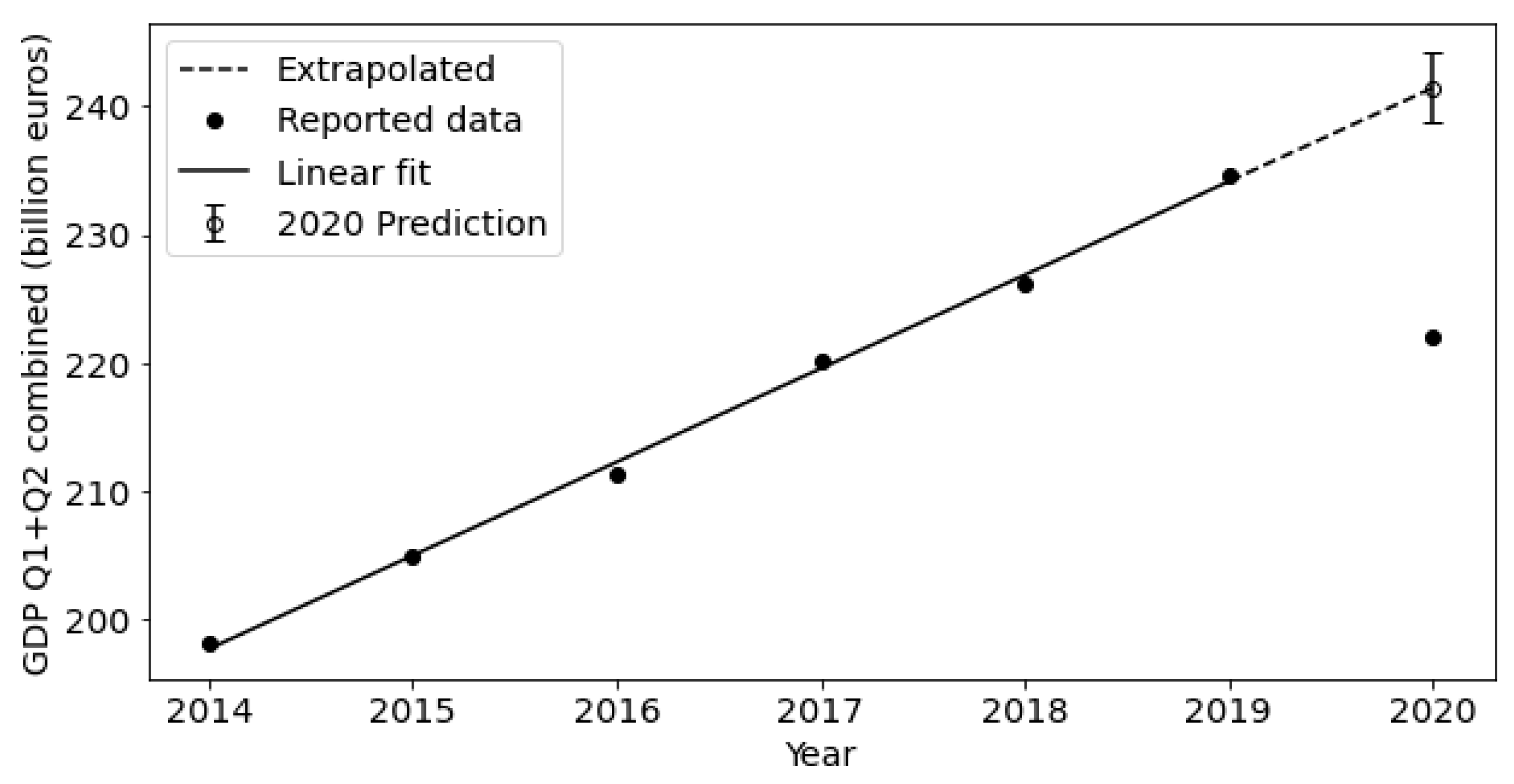
Figure 5.
Cumulative number of deaths simulated by means of the De Vischer model [35] for the following scenarios: no mitigation (red), modest mask-wearing effect (green), strong mask-wearing effect (turquoise), lockdown (blue). The numbers on the right correspond to the simulated total number of deaths for each scenario at the end of June 2020.

Table 1.
Quarterly values (in billion EUR) of Belgium’s gross domestic product for 2014–2020, as reported by the National Bank of Belgium [27].
Table 1.
Quarterly values (in billion EUR) of Belgium’s gross domestic product for 2014–2020, as reported by the National Bank of Belgium [27].
| 2014 | 2015 | 2016 | 2017 | 2018 | 2019 | 2020 | |
|---|---|---|---|---|---|---|---|
| Q1 | 97.1 | 100.1 | 102.4 | 107.7 | 110.3 | 114.7 | 116.3 |
| Q2 | 101.0 | 104.9 | 108.9 | 112.5 | 116.0 | 119.9 | 105.7 |
| Q1 + Q2 | 198.2 | 205.0 | 211.3 | 220.2 | 226.3 | 234.6 | 222.0 |
Disclaimer/Publisher’s Note: The statements, opinions and data contained in all publications are solely those of the individual author(s) and contributor(s) and not of MDPI and/or the editor(s). MDPI and/or the editor(s) disclaim responsibility for any injury to people or property resulting from any ideas, methods, instructions or products referred to in the content. |
© 2024 by the author. Licensee MDPI, Basel, Switzerland. This article is an open access article distributed under the terms and conditions of the Creative Commons Attribution (CC BY) license (https://creativecommons.org/licenses/by/4.0/).
Share and Cite
MDPI and ACS Style
De Ridder, K. Assessing the Value of a Human Life in Heat-Related Mortality: Lessons from COVID-19 in Belgium. Climate 2024, 12, 129. https://doi.org/10.3390/cli12090129
AMA Style
De Ridder K. Assessing the Value of a Human Life in Heat-Related Mortality: Lessons from COVID-19 in Belgium. Climate. 2024; 12(9):129. https://doi.org/10.3390/cli12090129
Chicago/Turabian StyleDe Ridder, Koen. 2024. "Assessing the Value of a Human Life in Heat-Related Mortality: Lessons from COVID-19 in Belgium" Climate 12, no. 9: 129. https://doi.org/10.3390/cli12090129
Note that from the first issue of 2016, this journal uses article numbers instead of page numbers. See further details here.