1. Introduction
Over the last few decades, data collected by the National Center for Atmospheric Research (NCAR) Electra Doppler Radar (ELDORA) has increased our understanding of a variety of weather phenomena ranging from tropical cyclones, to convective initiation, to tornadic thunderstorms, as well as mesoscale convective systems. The retirement of ELDORA in 2013 created a hard-to-fill gap in airborne radar capabilities that are available to the university research community. The Airborne Phased Array Radar (APAR) aboard the NCAR C-130 is designed to replace ELDORA and will soon be available for research flights. APAR’s dual-polarization radar will allow the atmosphere to be sampled at a higher spatial and temporal resolution and help probe deeper into storms.
The need for a tool to reduce the amount of time needed to process Doppler radar data while still producing a quality-controlled (QC’d) dataset has only been amplified by APAR’s much larger data stream. Radar data by their very nature contain both weather and non-weather echoes and can only be effectively used once the non-weather echoes are removed and the resulting weather echoes are QC’d. The QC process includes the use of airborne navigation and pointing angle corrections (Testud et al. [
1], Bosart et al. [
2]) followed by interactive data editing. NCAR’s SOLO software (Oye et al. [
3]) is the most widely used interactive data editing software. However, using NCAR’s SOLO software can be a hindrance for some researchers new to airborne radar data processing because of the time and training required to properly identify non-weather radar echoes. In addition, there is little documentation on how to effectively use SOLO software to properly edit radar data in general and specifically airborne radar data.
Employing NCAR’s SOLO software requires a significant amount of time even for experienced radar meteorologists, with rough estimates of up to 30 min to edit a single radar scan. By using this method, interactive editing of 10 min worth of ELDORA radar data could take up to 240 h. Bell et al. [
4] documented the characteristics of non-weather echoes captured using airborne Doppler radar and designed an algorithm to pre-process airborne Doppler radar data. The algorithm both reduced the “experience level” needed by the meteorologist to assess non-weather echoes and also reduced the time required to QC the datasets. Bell et al. [
4] validated the algorithm by examining the impact the algorithm had on derived products such as dual-Doppler synthesis and radar data assimilation. The authors [
4] used four Electra Doppler Radar (ELDORA) datasets that were first interactively edited by different experienced radar meteorologists and next applied their automated QC algorithm.They then conducted an analysis of the impacts of the automated QC algorithm on dual-Doppler retrievals using the methodology described in [
5] using data from T-PARC. The SOLO automated QC values used in this study are listed in
Table 1, and with the exception of the extra-low thresholds, they are the same as used in Bell et al. [
5]. Differences between the original analysis by Wakimoto et al. [
6] revealed minor variances between the low and medium algorithms, while the high algorithm produced larger differences. Those larger differences were the result of low dBZ echoes present in the interactive analysis, which were removed by the automated QC algorithm. The differences in root mean square (RMS) were less than
across the entire domain.
Bell et al. [
4] demonstrated that an automated process could reduce the amount of time needed to process Doppler radar data while still producing a QC’d dataset. A more quantitative analysis could provide further substantiation. Perturbation pressure retrievals developed by Gal-Chen [
7] (and tested by Pasken and Lin [
8]) would provide a more stringent test. Perturbation pressure retrievals require finding the second and third derivatives of the wind field, unlike a kinematic analysis that requires only the first derivative of the wind field. For the perturbation pressure retrieval to produce a meaningful and consistent pressure field, the wind fields used in the retrieval must not only be kinematically consistent, but must also conserve momentum in the x, y and z directions. The momentum checks (
) values, using the perturbation retrieval methodology and computed at each level, provide a measure of how well the momentum and pressure gradients are conserved. Thus, perturbation pressure retrieval provides a quantitative measure of the quality of the pressure retrieval. Low momentum check values (
) indicate quality pressure retrieval, while momentum check values larger than 0.5 indicate retrieval problems. Values > 0.5 can still provide useful information. Momentum check values cannot be lower than 0.25 (Gal-Chen [
7]). Comparing the momentum check values from the hand analysis against those from the automated algorithm would provide a quantitative test of how well the automated analysis performed.
The tests by Schmitz [
9] using perturbation pressure retrievals with data from the BAMEX field campaign indicated that the
produced by the automated QC algorithm was as good, if not better, than the interactive analysis. Although Schmitz [
9] performed these tests with ELDORA data from several time periods during a single BAMEX flight, the tests were limited to a single BAMEX case. A more thorough comparison using a similar methodology applied to other ELDORA cases should provide a more quantitative answer to performance of the automated algorithm. Using the automated QC process employed by Schmitz (2010) with data from the same four cases used in [
4] would stress the automated algorithm more thoroughly than the single case tested by Schmitz [
9]. Further, this allows for a direct comparison between the results from Bell et al. [
4] with the results of this study.
The perturbation pressure retrievals provided a quantitative measure of the quality of the pressure retrieval in the form of the momentum check values, but as noted earlier, low momentum check values do not ensure that the resulting perturbation fields produce physically meaningfully values. The resulting perturbation pressure fields need to be examined to ensure that numerically and physically meaningful results are produced. To quantitatively compare the perturbation pressure fields from the hand analysis to the automated analysis, computing the correlation coefficients of the perturbation pressure field would provide an additional test of the automated algorithm.
The focus of this article is to demonstrate the ability of the automated SOLO algorithm to simplify the QC process, reduce the amount of time needed to process a airborne radar dataset and to help researchers new to airborne radar effectively use the resource.
2. Methodology
Gal-Chen [
7] proposed that perturbation pressures, densities and temperatures could be recovered from the Doppler radar data via the anelastic form of the Navier–Stokes equation, given the three-dimensional wind field over time. Pasken and Lin [
8] tested the method using dual-Doppler radar data collected by the National Severe Storms Laboratory in 1974. Although the perturbation pressure fields recovered by Pasken and Lin [
8] were consistent with the conceptual models of the storm, an independent verification of the perturbation pressure fields was not possible. The use of finite differences, scanning rates and parameterization of the turbulence fields contribute to errors in the recovered perturbation fields. The size of these errors in any particular perturbation field needs to be assessed in some fashion. As pointed out by Gal-Chen and Kropfli [
10] that while the kinematic fields generated from a multiple Doppler analysis are likely to be accurate enough to create qualitatively correct divergence and vorticity fields, derivatives of the velocity fields might not be accurate enough to create the perturbation pressure fields. Thus, some method of determining the reliability of the recovered pressure and temperature fields is necessary. Gal-Chen and Kropfli [
10] suggested three methods for indirect verification of the perturbation pressure fields: (1) momentum checking, (2) time continuity and (3) physical plausibility. Gal-Chen [
7] noted that the equations used to recover the perturbation fields were overdetermined and had a solution only if
If both the wind field had no errors and the parameterization of friction was exact, then Equation (
1) would be satisfied. Unfortunately, the wind field has errors, and friction is not exactly accounted for. As such, the perturbation fields also contain errors, which can be quite large. The perturbation fields can be computed in terms of a least squares fit by minimizing
A measure of the least squares fit can be found from
where
;
;
storm relative u wind component;
storm relative v wind component;
;
;
u component of storm motion;
v component of storm motion;
hydrostatic adiabatic density.
When momentum check = 0, the fit is perfect. If, on the other hand,
F and
G are random values, then
. Hane and Ray [
11] pointed out that even when
, the perturbation fields can still contain useful information, provided the time continuity and physical plausibility conditions are also met. However, it is also possible that even if
F and
G are perfect, the use of finite differences and the inability to recover waves due to resolution problems can yield a non-zero momentum check value. Thus, the value of momentum check should be considered as a relative measure of the goodness-of-fit of the perturbation field gradients and the dynamic fields.
Comparing the values of momentum check between the hand-edited and automated edited perturbation fields provides a measure of the quality of the automated editing process. However, it is possible that the automated editing of the data could produce comparable momentum check values, while the perturbation fields bear no resemblance to hand-edited fields. To ensure that the perturbation fields from the hand and automated editing produce similar fields, the Pearson correlation coefficient between the two fields was computed. Provided the perturbation fields make physical sense, the correlation coefficients are approximately one and the momentum check values are comparable, it can be assumed that the automated editing produces results as good as the hand-editing analysis.
Comparing the momentum check values and correlation coefficients multiple times from the same storm would provide a means of testing the time continuity constraint discussed by Gel-Chen and Kropfli [
10]. Combing all three tests with momentum check values, correlation coefficients and continuity across analysis gives a quantitative test of the automated quality control technique.
The radar data used in these experiments were collected during the Verification of the Origins of Rotation in Tornadoes Experiment (VORTEX), the Bow Echo and Mesoscale Convective Vortex Experiment (BAMEX), Hurricane Rainband and Intensity Change Experiment (RAINEX) and Thorpex-Pacific Asian Regional Campaign (T-PARC) field experiments. The VORTEX dataset was discussed in Wakimoto et al.’s work [
12], while the BAMEX case was discussed in [
13]. Both represent different types of mid-latitude continental convection. The RAINEX dataset was discussed in [
14] and T-PARC by Bell and Montgomery [
5], both of which represent cases of tropical oceanic systems in different stages of development. In each case, the hand-edited dataset was obtained from the authors and the three-dimensional wind field was computed using the method described in Gamache’s paper [
15]. The perturbation pressure fields were then computed using the method described by Pasken and Lin [
8]. The raw radar datasets were then processed via the automated QC algorithm, and the three-dimensional wind and perturbation pressure fields were recomputed. In each case, the momentum check values were computed.
Since an observed perturbation pressure field does not exist, hand-edited perturbation pressure fields were considered to be the “true” values and the perturbation computed from the automated QC algorithm was compared to the hand-edited values. When comparing results from different systems, care must be taken as the hand-edited wind fields were performed by different radar meteorologists. Also, one should note that the goals of each experiment were different.
Unlike other radar QC tools, SOLO has both the ability to manually edit the raw radar data and to use a scripting language to simplify repetitive actions applied to the radar data. Using this scripting language, Bell et al. [
4] created a series of editing scripts that can be used as a starting point for further interactive editing within the SOLO environment.
3. Results
As noted by Gal-Chen and Kropfli [
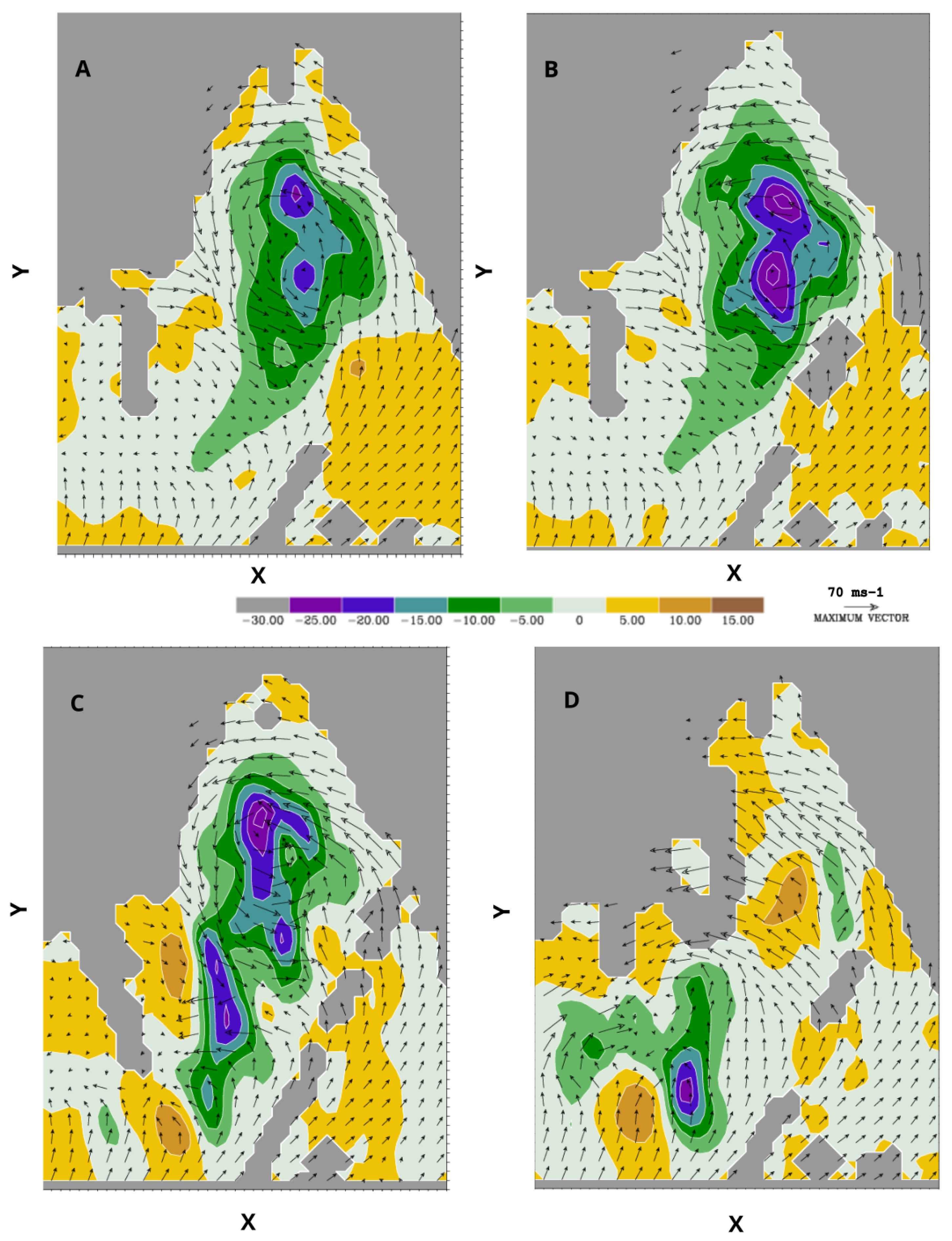
10], the first test is whether or not the resultant perturbation pressure field makes physical sense. For the BAMEX case (
Figure 1), the high automated QC algorithm did not produce results that resembled the hand analysis, so it no longer remained under consideration. Note that in this and in the following horizontal perturbation pressure figures, the vertical and horizontal grid spacing is 500 m and every other wind vector has been removed. The results of the medium automated QC algorithm also did not produce realistic results. The low automated QC algorithm produced results that were closer to “truth”, but with distorted features in the perturbation pressure field. In an attempt to improve the automated QC algorithm, the portion of the algorithm that treat “freckles” was removed and the resulting analysis method was called extra-low. The extra-low analysis documented lower (less) negative perturbations pressures as well as a much greater total of negative perturbation pressures. Wind fields also showed similar flow around the dual cores of negative perturbation pressures. The wind field in the low case is significantly different from both the hand-edited and extra-low automated QC wind fields. This accounts for the difference in the perturbation pressure field. The medium automated QC wind removes the twin circulations’ centers entirely, resulting in a perturbation pressure field that does not resemble the hand analysis.
Figure 2 shows the differences in momentum check values between the automated QC algorithm and the hand-edited analysis. Note that negative values indicate that the automated QC values are lower and hence are better than the hand analysis. Although the low automated QC analysis has lower momentum check values at some levels, the extra-low analysis is more consistent throughout the vertical. Note that in this and the following figures, the curves may overlap such that they appear as one line. The differences between the extra-low analysis and the hand analysis are small. Although at 1.75 km the difference is 0.11, the other differences are between 0 and 0.05. These small differences between the hand analyses indicate that the automated QC analysis reproduces the perturbation pressure fields with nearly the same quality as the hand analysis. As noted above the momentum check values do not necessarily indicate a quality analysis. However, in this context, the fact that the values from the automated analysis are the same as or slightly better than those of the hand analysis indicates that the automated QC analysis, incorporating the “freckels” modification, is an acceptable alternative to a hand analysis. Further, since these results are for the automated analysis only, additional tuning by a radar meteorologist would most likely produce a better analysis in a region where the vortex is most prominent.
Figure 3 and
Figure 4 are the perturbation pressure fields, correlation coefficients and momentum check differences for the Garden City/VORTEX case. The low automated QC analysis shows large differences between the hand and automated analyses. This is likely due to the automated QC analysis failing to retain the larger radial velocities near the hand-analysis pressure minimum. The resulting lower wind speeds distorted the pressure recovery, resulting in a much larger minimum. On the other hand, the medium and high automated QC analyses produce perturbation pressure fields that are qualitatively similar to the hand analysis. The similarity is borne out when the correlation coefficients are examined. With the exception of the first analysis level near the ground, all the correlation coefficients are greater than 0.9, indicating a very close match between the hand analysis and the automated QC analysis. As with the correlation coefficients, the momentum check values are slightly better for the automated QC analysis than for the hand analysis. As noted earlier, the hand analysis was conducted by a radar meteorologist using his or her own subjective understanding of the meteorology in producing the radial velocity and reflectivity fields. The automated analysis applies a similar but objective set of rules to the radial velocity and reflectivity fields. The application of the objective rules result in slightly better generated perturbation pressures fields. However, they are not readily visible in the perturbation pressure fields but are reflected in the momentum check values. This effect is most prominent in the low to middle altitudes where the largest changes in the radial velocities and reflectivities occur. The Garden City/VORTEX case is an example of how well the automated QC process can work. The BAMEX case, with its very strong vortex, stressed the automated QC process. It did not recover the radial velocities as well as a hand analysis.
The Rita-RAINEX experiment results, shown in
Figure 5 and
Figure 6, are the opposite of the Garden City/VORTEX case. In the Rita-RAINEX case, the low automated QC produced a better-quality analysis than the hand analysis. The medium and high automated QC analyses remove the larger radial velocities from the radar, resulting in changes in the speed and direction of the computed wind field. These changes in the wind field resulted in a much larger deficit in the upper right-hand corner of the perturbation pressure field than that found in the hand analysis. As expected, the very lowest levels have the largest gradients in reflectivity and radial velocities and, as a result, have the poorest correlations. These correlations rise above 0.9 between roughly 2.4 km and 6.0 km. The low automated QC analysis has correlation coefficients that are slightly better than the medium and high automated QC analyses. The momentum check differences are nearly zero with the exception of the uppermost level, where the limited number of samples and very small changes in both the radial velocities and reflectivities retained by the analysis have a very large effect.
The results of the Hagupit-TPARC experiment presented are an example of how well the automated QC analysis can perform. The results of the analysis for the Hagupit-TPARC case are shown in
Figure 7 and
Figure 8. The perturbation pressure fields are very similar; the only difference is in the magnitudes of the pressure deficits/excesses rather than locations. The low automated QC analysis matches the hand analysis more closely. However, the differences between the low, medium and high analyses are small, amounting to less than 0.1 mb. The correlation coefficients are all above 0.865 (note the scale change between
Figure 8 and the previous correlation coefficient graphs). The high and medium automated QC analyses likely drop to 0.865 at the lowest level because more of the data are removed at the lowest level by the medium and high automated QC analyses, but not the low automated analysis. The momentum check plot shows that there is very little difference between analysis methods as is to be expected given the very close match between the different analysis methods.
As noted by Gal-Chen and Kropfli [
10], another indirect method used in verifying the results of a perturbation pressure analysis is a time continuity check. Unfortunately, a comparison over multiple time periods of a hand analysis versus automated QC for all the above cases was not possible, as hand analyses by the original authors were not available.
To conduct a time continuity check of automated QC analysis of BAMEX case, data from Schmitz [
9] at 05:20 UTC, 05:30 UTC, 05:40 UTC and 05:50 UTC were used to compare the momentum check to provide insight into the consistentency of the automated QC analysis process.
Figure 9 is a plot of the momentum check values for the extra-low, low and medium automated QC at 05:20 UTC, 05:30 UTC, 05:40 UTC and 05:50 UTC, respectively, with a fourth-order curve fit. For the extra-low case (
Figure 9A), with the exception of the 05:40 UTC, the momentum check values for the other time periods show the same overall pattern with only small variations in the actual momentum check values. The similar overall pattern and small variation in momentum check values in the 05:20Z, 05:30Z and 05:50Z analyses imply that the automated QC analysis process can produce a consistent analysis. This is further documented by the smooth curve fit lying in between the four time periods. The 05:40UT time [
9] was able to use the hand-edited results as reference but is not as representative of the automated QC analysis as other time periods.
Figure 9B shows the plot of the values for the low automated QC for 05:20Z UTC, 05:30 UTC, 05:40 UTC and 05:50 UTC. Note that the 05:20 UTC and 05:30 UTC curves overlap. As with the extra-low automated QC analysis, the 05:40 UTC has a different shape and a larger range of momentum check values. However, the 05:20 UTC, 05:30 UTC and 05:50 UTC automated QC momentum check values have a much smaller range and the shapes of the momentum check curves match more closely than the low automated analysis. This implies that the medium automated QC analysis produces a much more consistent time continuity and has a better time consistency than the low automated QC analysis. The inconsistent 05:40 UTC analysis has a similar shape for the momentum check values for both the extra-low and low automated QC analysis, indicating that the problem is with the 05:40 UTC data and not the automated QC analysis. As a result, the curve fit shows higher variation than the low case. The time continuity plot for the high automated QC analysis is presented in
Figure 9C. The momentum check values for the medium automated QC analysis show an increased variation between times than either the extra-low or low automated QC analysis methods. The curve fit shows a similar curve fit to the low case until the upper levels, where it is 05:50 UTC. This may be the result of the aggressive removal of data used in the medium automated QC analysis method. The variations in time continuity results between the extra-low, low and medium are comparable to those seen in the correlation coefficients, momentum check values and a simple visual comparison of the perturbation pressure fields.


