Assessing Climate Change Impacts on Combined Sewer Overflows: A Modelling Perspective

Abstract

The study examines the impacts of climate change on the operation and capacity of the combined sewer network in the historic center of Thessaloniki, Greece. Rainfall data from three high-resolution Regional Climate Models (RCMs), namely (a) the Cosmo climate model (CCLM), (b) the regional atmospheric climate model (RACMO) and (c) the regional model (REMO), from the MED-CORDEX initiative with future estimations based on Representative Concentration Pathway (RCP) 4.5, are first corrected for bias based on existing measurements in the study area. Intensity–duration–frequency (IDF) curves are then constructed for future data using a temporal downscaling approach based on the scaling of the Generalized Extreme Value (GEV) distribution to derive the relationships between daily and sub-daily precipitation. Projected rainfall events associated with various return periods are subsequently developed and utilized as input parameters for the hydrologic–hydraulic model. The simulation results for each return period are compared with those of the current climate, and the projections from various RCMs are ranked according to their impact on the combined sewer network and overflow volumes. In the short term (2020–2060), the CCLM and REMO project a decrease in CSO volumes compared to current conditions, while the RACMO predicts an increase, highlighting uncertainties in short-term climate projections. In the long term (2060–2100), all models indicate a rise in combined sewer overflow volumes, with CCLM showing the most significant increase, suggesting escalating pressure on urban drainage systems due to more intense rainfall events. Based on these findings, it is essential to adopt mitigation strategies, such as nature-based solutions, to reduce peak flows within the network and alleviate the risk of flooding.

1. Introduction

A number of latest studies conducted by the Intergovernmental Panel on Climate Change (IPCC, 2014) reported evidence for changes in the occurrence of certain meteorological events during the 21st century. Regarding precipitation extremes in Europe, increased precipitation intensity in a future climate was one of the model results of most recent studies [1,2,3,4,5,6]. The IPCC’s assessments heavily relied on global circulation models (GCMs), which are large-scale mechanistic models of the global atmosphere that are inherently coupled with ocean systems. Regional Climate Models (RCMs) are forced by the output of the GCMs as initial or boundary conditions and simulate regional climates with a finer resolution, enhancing the spatial resolution of climatic projections. In previous years, different RCMs were used to produce high-resolution climate scenario calculations on the European scale (e.g., EU-projects PRUDENCE, ENSEMBLES, and CORDEX), including the entire Mediterranean basin [7,8,9].

Future climate projections produced by climate models (GCMs and RCMs) are still subject to large uncertainties that possibly originated from three major sources such as the emission uncertainty, the model uncertainty reflecting the limited understanding of the different atmospheric processes and their representation in the climatic models, as well as the uncertainty due to natural variability [10]. Especially when using RCM data, the drivers of uncertainty increase, as the model resolution, the forcing lateral conditions, and physical parameterizations [11,12] induce more bias and variance in the results. Therefore, the aforementioned uncertainty sources should be considered when assessing the impacts of climate change on different domains so that the estimation process is more reliable and robust. Model uncertainty can be considered by creating a multi-model ensemble, which consists of climate models that are ideally structurally independent. Kendon et al. [13] combined climate models through a multi-model ensemble to produce more reliable and consistent climate projections, suggesting the use of at least three components to estimate changes in precipitation extremes.

Different scales (spatial and temporal) between RCMs and local measuring gauges or local urban drainage systems can have significant effects and produce inaccuracies on the precipitation process or the different sewer processes [14,15]. The aforementioned arguments may necessitate the use of dynamic or statistical downscaling methods to reduce the effects of the coarse scales of climate models on precipitation and urban drainage studies. Statistical downscaling includes methods that are quite easy to apply, are not time consuming, and are considered rather efficient. This category of methods includes statistical models to transfer the “predictor” variables, which are available on a coarse grid, to the “predictand” variable, corresponding to finer spatial scales. Statistical downscaling methods include the construction of empirical transfer functions, weather typing models, or stochastic modeling methods [16]. The former methods create and utilize transfer functions between the coarse scale variable of the climatic model and the smaller scale variable. Bias correction methods include the development of transfer functions between the cumulative distribution functions of the climate model and observed data. Bias represents the error component of the climate model that is independent of time [17]. Among the bias correction techniques, recent studies mainly using precipitation and temperature data indicated that the quantile mapping methods are the most efficient, even for the most extreme part of the distribution of the studied variables [18,19,20,21]. Gudmundsson et al. [22] reviewed and classified bias correction methods using observations of a large number of precipitation stations in Norway to systematically reduce biases in RCM precipitation projections. Teutschbein and Seibert [23] reviewed and evaluated different bias correction methods for hydrological climate change impact studies. Tani and Gobiet [20] developed an extended version of the quantile mapping approach to provide more reliable bias-corrected precipitation extremes by combining the advantages of nonparametric methods and extreme value theory. Chandra and Papalexiou [24] introduced a semi-parametric approach for correcting daily precipitation for bias, providing good results for extreme quantiles. Holthuijzen et al. [21] developed a combined approach to adjust biases in precipitation, featuring a strong linear modification for extreme events.

Another significant issue that should be considered refers to the fact that hydro-meteorological variables, such as precipitation, resulting from climate models, are not, in general, available in time series with fine temporal resolution (e.g., 10 min to 1 h time steps). However, these time scales are essential for studying and estimating the effects of climate change, especially on medium or small catchment areas. Temporal downscaling and temporal disaggregation are used to overcome such difficulty. Temporal downscaling usually refers to the generation of data of high temporal resolution by means of statistical techniques, most commonly stochastic models, which are calibrated using information on the statics of data from lower resolution temporal scales. The most used downscaling approaches are statistical downscaling methods. Nguyen et al. [25] proposed a statistical temporal downscaling method which is based on the scaling Generalized Extreme Value (GEV) distribution to describe the relationships between daily and sub-daily extreme precipitation. Terti et al. [26] evaluated the suitability of the abovementioned approach for determining the distribution of short-duration extreme rainfall in Thessaloniki, Greece. Ghanmi et al. [27] used the simple scale invariance concept to statistically downscale daily rainfall in northern Tunisia to sub-daily amounts. Yeo et al. [28] used GEV scaling to estimate sub-daily annual maximum precipitation from daily values and applied their methodology to available data from Quebec, Canada, and Seoul, South Korea. Galiatsatou and Iliadis [29] applied a simple scaling approach based on the GEV distribution to assess short-duration rainfall extremes at ungauged sites transferring information from gauged ones with a relatively homogeneous extreme rainfall climate. Iliadis et al. [30] used a GEV scaling approach on daily rainfall extremes that were assessed from a long-term time series to estimate fine temporal-scale extreme events in Thessaloniki, Greece.

Locally derived intensity–duration–frequency (IDF) relationships are commonly applied in engineering planning and management, including flood defense systems, infrastructure, and mitigation initiatives. These curves are developed for various recurrence intervals, illustrating how rainfall intensity changes over time. Theoretical probability distribution functions are fitted to annual maximum rainfall intensities of particular durations ranging from shorter ones, e.g., 5 min, to daily precipitation events. These curves are currently designed under the assumption of stationarity [31,32,33], namely the hypothesis that the occurrence probability of precipitation events will remain unaltered or will not exhibit significant changes in time, mainly due to the lack of predictability on details of possible future changes. However, hydro-meteorological patterns, particularly at extreme levels, demonstrate nonstationary behavior. Key factors contributing to these changes include natural climate fluctuations, human-induced alterations in watershed hydrology, and the impacts of climate change [34,35]. Yan et al. [36] reviewed the literature on updating IDF curves under climate change, mainly emphasizing covariate-based distributions for modeling extremes. Martel et al. [37] studied changes in extreme precipitation and related sources of uncertainty. Schlef et al. [38] presented a review on current knowledge and research on nonstationary IDF curves. Nonstationary IDF curves are usually constructed under the assumption of covariate-based modeling or simulated precipitation from RCMs or GCMs. In the latter case, precipitation extremes are obtained over historical and future periods (projections) from a number of climate models (RCMs or GCMs). However, there is currently an ongoing discussion on whether and to what degree nonstationarity should be addressed when designing for hydroclimatic extremes, mainly focusing on uncertainty, model complexity, and data limitation issues [39,40].

Considering that there is increasing evidence of climate change associated with destructive extreme events of higher intensity and frequency, combined with the deterioration process of the sewer network and the rapid growth of cities, an increase is expected in the number of people and properties in urban areas affected by the harmful effects of urban stormwater. In this context, urban drainage infrastructures are unlikely to be adequate in the future in most cities worldwide, because their design relied upon historical precipitation data which ignored climatic variability. Kourtis and Tsihrintzis [41] reviewed state-of-the-art scientific approaches for the adaptation of urban drainage networks to climate change, discussing climate change impacts on precipitation, IDF curves, flooding, and urban drainage, and defined a novel approach for assessing urban drainage network adaptation to climate change and other drivers. Galiatsatou and Iliadis [29] introduced a methodological framework for designing urban drainage networks under climate change conditions, considering the nonstationarity of the extreme precipitation in the study area. Galiatsatou et al. [42] evaluated the performance of a sewer system under rainfall events of varying recurrence intervals and suggested measures (nature-based solutions) to reduce overflows.

In addition, surface runoff in combined sewer overflows (CSOs) can lead to the discharge of untreated wastewater, which poses significant health risks by contaminating drinking water and recreational areas with harmful pathogens and pollutants [43,44]. This not only threatens human health but also causes environmental damage by polluting water bodies, disrupting aquatic ecosystems, and contributing to eutrophication and habitat destruction [45].

In this framework, this study investigates the effects of climate change on the operation and capacity of the combined sewer network in the historic center of Thessaloniki, Greece, using high-resolution rainfall data from three Regional Climate Models (RCMs). The novelty of the research lies in the use of a temporal downscaling method based on the Generalized Extreme Value (GEV) distribution to develop future intensity–duration–frequency (IDF) curves for sub-daily precipitation. Furthermore, this study offers a detailed comparison of projected CSO volumes across different RCMs, emphasizing the varying impacts on the sewer system and overflow volumes under both near-term and long-term climate scenarios.

2. Materials and Methods

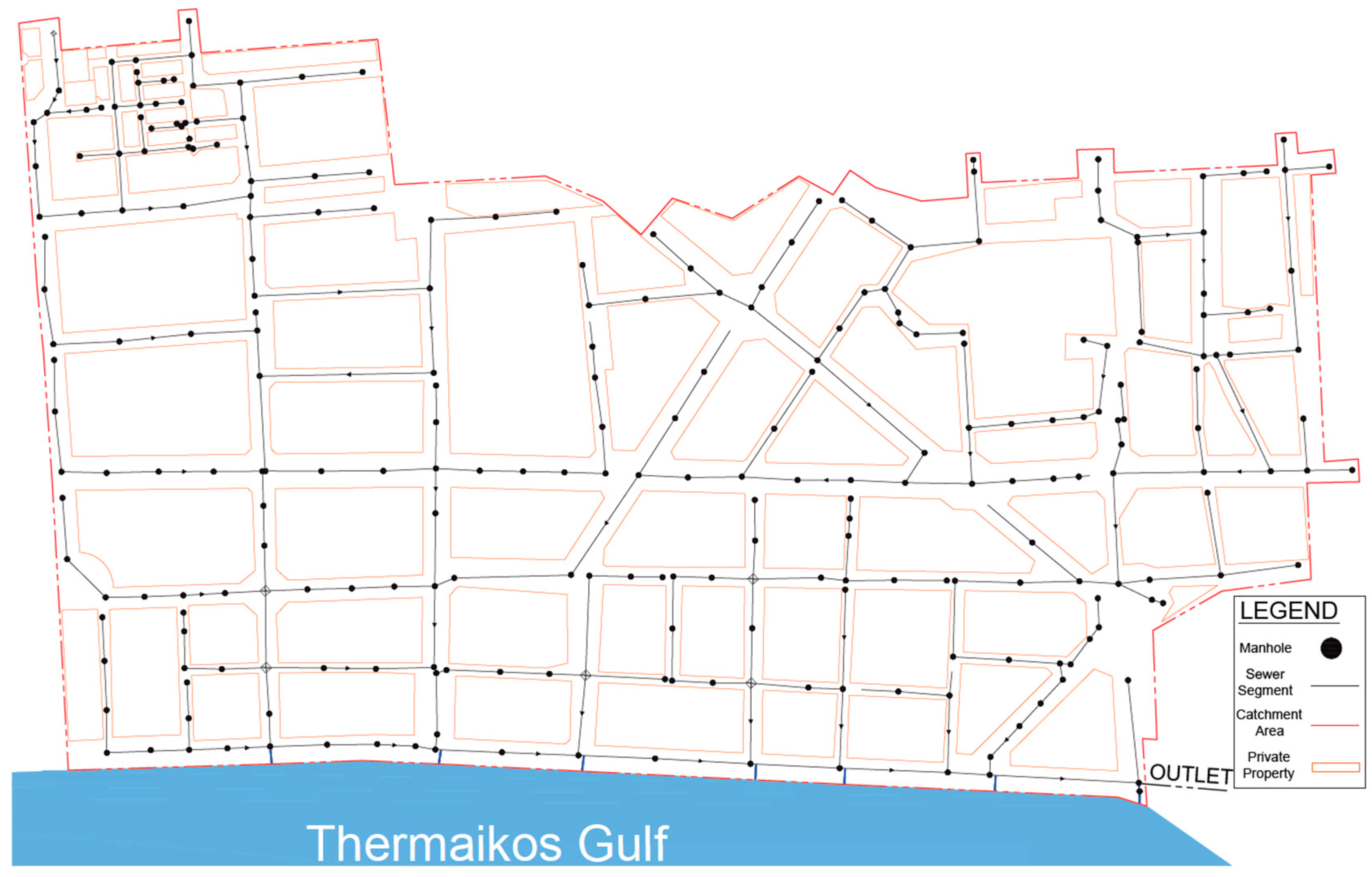
2.1. Study Area

This study examines the historic district of Thessaloniki, Greece. Thessaloniki has a population exceeding one million, with its central area being particularly dense. The average yearly rainfall between 1960 and 2020 measured 445.7 mm. During this period, monthly precipitation varied, with the lowest recorded at 21.1 mm in August and the highest at 54.5 mm in December. The study site extends from Aristotelous Street in the west to Aggelaki Street in the east, while its northern boundary follows Egnatia and Svolou streets, and the southern edge runs along Leoforos Nikis by the coast. The drainage area of the system is estimated at 40 ha and is depicted in Figure 1.

2.2. Climate Data Assessment and Downscaling Methodology

Historical precipitation measurements were obtained from the meteorological station (MS) of the Aristotle University of Thessaloniki (AUTH) which is located near the study area. These historical records covered the period from October 1965 to September 2005. The AUTH station has been widely recognized for its long-term, high-quality data collection, making it a reliable source for climatological analysis and model evaluation.

Future precipitation projections used in this study were sourced from the EURO-CORDEX coordinated downscaling experiment [46], an initiative under the CORDEX framework. This dataset provides high-resolution regional climate simulations, ensuring the robustness of climate projections across Europe. For this analysis, monthly precipitation projections were derived from three distinct Regional Climate Models (RCMs), as presented in

Table 1. List with the 3 EURO-CORDEX sets of simulations used in the present study.

	Institute_id	RCM	Driving GCM	Realization
1	CLMcom	CCLM4-8-17.v1	CLMcom.ICHEC-EC-EARTH	r12i1p1
2	KNMI	RACMO22E.v1	KNMI.ICHEC-EC-EARTH	r12i1p1
3	MPI-CSC	REMO2009.v1	MPI-CSC.MPI-M-MPI-ESM-LR	r1i1p1

.

Each RCM provides a spatial resolution of 0.11o (approximately 12.5 km), offering a fine spatial grid suitable for local-scale climate impact studies. The future projections covered the period from October 2020 to September 2100 and were performed under the Representative Concentration Pathway (RCP) 4.5 scenario. This scenario represents an intermediate greenhouse gas emission pathway, where emissions peak around mid-century and then stabilize.

To ensure consistency and comparability, historical precipitation observations (1965–2005) were directly compared to the corresponding historical simulation outputs from the RCMs for the same period. Given the inherent biases present in raw precipitation outputs from RCMs, bias correction was necessary. The Bias Correction Quantile Mapping (BCQM) method was employed for this purpose utilizing the qmap package [22] in R. This statistical technique adjusts the cumulative distribution of modeled precipitation to align with that of observed precipitation, thereby addressing systematic discrepancies. The BCQM approach uses a non-linear transformation to model the quantile–quantile relationship between observed and simulated precipitation values. Specifically, the exponential tendency to an asymptote transformation function was applied, as described by Gudmundsson et al. [22]:

$${\widehat{X}}_o=(a+b\times X_m)(1-e^{-{\displaystyle \frac{\left(X_m-x\right)}{\tau }}})$$

(1)

where ${\widehat{X}}_o$ is the observed variable, X_m is the modeled variable, and a, b, x, and τ are the parameters.

The bias-corrected transformation function was subsequently applied to the future climatic projections to adjust for biases in the raw outputs of the climate models. To enable a more detailed analysis of future climatic trends, the projected period spanning from 2010 to 2100 was divided into two distinct 40-year intervals: 2020–2060, representing the short-term projection, and 2060–2100, representing the long-term projection. The mean annual precipitation and its associated standard deviation were computed for both the historical period and the future time intervals for each of the three climate models after bias correction.

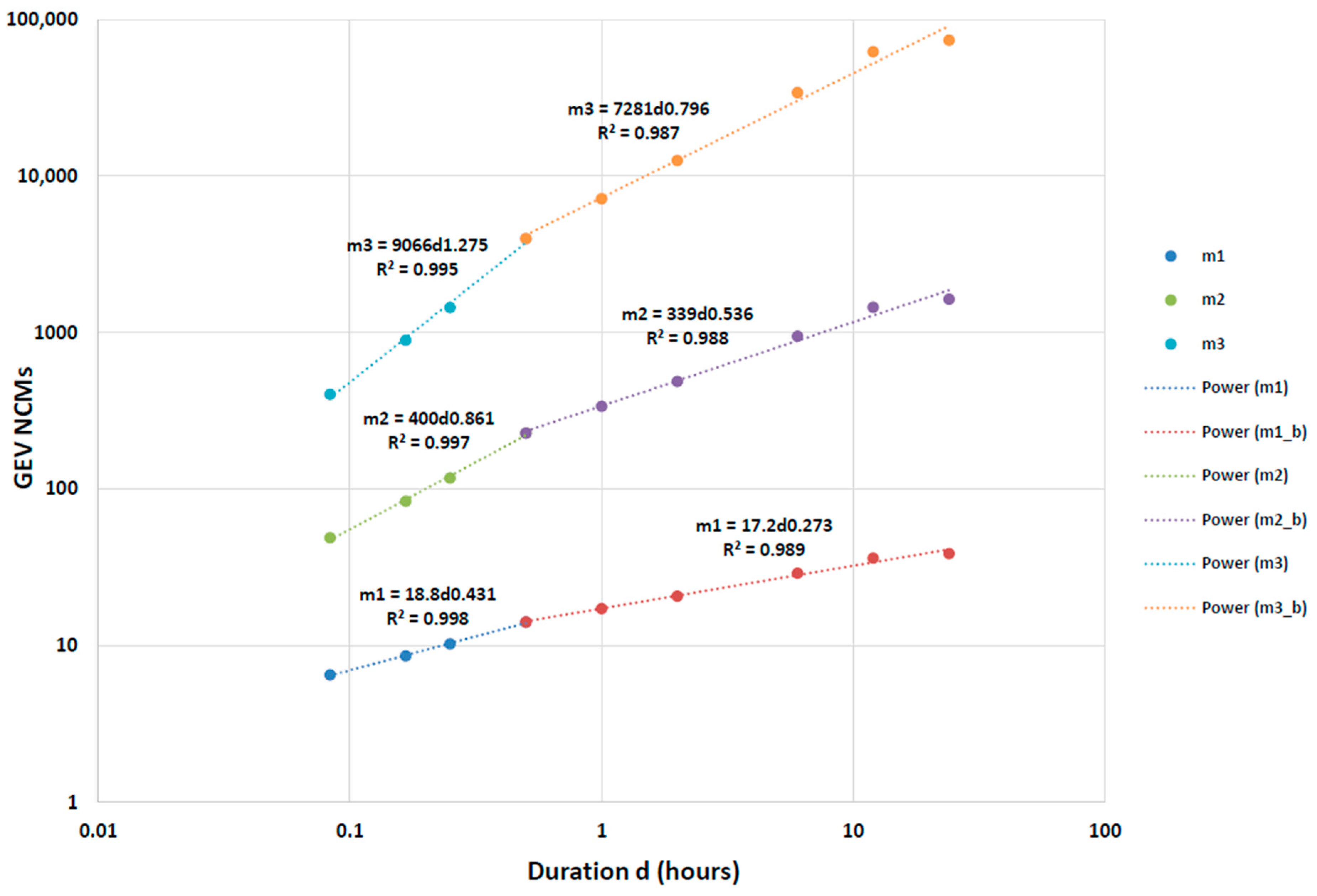
2.3. The Scaling GEV Model

The GEV distribution has been used in several scientific studies for modeling annual series of extreme rainfall, as it has been proven that it matches well the observed extreme values. The cumulative distribution function (CDF), G(x), for the GEV distribution is given as

$$G\left(x;\mu ,\sigma ,\xi \right)=\left\{\begin{array}{c}\exp \left\{-{\left[1+\xi {\displaystyle \frac{x-\mu }{\sigma }}\right]}^{-{\displaystyle \raisebox{1ex}{$1$}\!\left/ \!\raisebox{-1ex}{$\xi $}\right.}}\right\} \xi \ne 0\\ \exp \left[-\exp \left({\displaystyle \frac{x-\mu }{\sigma }}\right)\right] \xi =0\end{array}\right.$$

(2)

where μ, σ, and ξ are, respectively, the location, scale, and shape parameters, with the latter also determining its limiting behavior. When the shape parameter, ξ, is equal to zero the GEV distribution is equivalent to the Gumbel distribution, but when ξ is higher or lower than zero, the GEV corresponds to the Fréchet and the (reversed) Weibull distribution families, respectively. In this work, due to the small sample size of the annual maximum rainfall series (40-year maxima for all study periods and climate models), the three parameters are estimated using the method of L-moments [47,48]. For the random variable X with distribution function F, the theoretical L-moments λr + 1 with r = 0, 1, … are expressed as linear functions of the specific probability weighted moments (PWMs):

$$a_r=M_{\mathrm{1,0},r}=\mathrm{E}\left\{X{\left[1-F\left(X\right)\right]}^r\right\}$$

(3)

with the dimensionless L-moment ratios L-skewness, τ₃ = λ₃/λ₂, and L-kurtosis, τ₄ = λ₄/λ₂, calculated as functions of the L-scale, λ₂, and the third, λ₃, and fourth, λ₄, L-moments. Let a_r be the unbiased estimator of a_r for an ordered sample x_1:n ≤ … ≤x_n:n [45]:

$${\mathrm{a}}_{\mathrm{r}}={\displaystyle \frac{1}{n}} {\sum }_{i=1}^n\left(\begin{array}{c}n-i\\ r\end{array}\right)x_{i:n}{\left(\begin{array}{c}n-1\\ r\end{array}\right)}^{-1}, r=0, 1,\dots , n-1$$

(4)

with the unbiased sample L-skewness, t₃ = l₃/l₂, and L-kurtosis, t₄ = l₄/l₂, calculated as functions of the sample L-scale, l₂, and the third, l₃, and fourth, l₄, sample L-moments, respectively. If the L-moment estimation method results in a quite low estimate of the shape parameter (estimate close to −0.5) of the extreme precipitation process for a certain time interval and climate realization scenario, the maximum likelihood estimation (MLE) procedure is also applied to estimate the GEV parameters [49,50].

After the parameters’ estimation, the quantiles X_Τ for each return period T can be calculated as follows:

$$X_T=\left\{\begin{array}{c}\mu -{\displaystyle \frac{\sigma }{\xi }}\left\{1-{\left[-\mathrm{l}\mathrm{n}\left(1-{\displaystyle \frac{1}{T}}\right)\right]}^{-\xi }\right\} \xi \ne 0\\ \mu -\sigma \ln \left[-\mathrm{l}\mathrm{n}\left(1-{\displaystyle \frac{1}{T}}\right)\right] \xi =0\end{array}\right.$$

(5)

It can be shown that the k-th order of non-central moments (NCMs), m_k, can be expressed as a function of the three GEV parameters as

$$m_k={\sum }_{i=0}^k\left(\begin{array}{c}k\\ i\end{array}\right){\left(-1\right)}^i{\left(-{\displaystyle \frac{\sigma }{\xi }}\right)}^{k-i}\Gamma \left(1-i\xi \right)$$

(6)

For k = 1, 2, and 3, Equation (5) can be written as follows:

$$m_k={\left(\mu -{\displaystyle \frac{\sigma }{\xi }}\right)}^k+{\left(-1\right)}^k{\left(-{\displaystyle \frac{\sigma }{\xi }}\right)}^k\Gamma \left(1-k\xi \right)+k{\sum }_{i=1}^{k-1}{\left(-1\right)}^i{\left(-{\displaystyle \frac{\sigma }{\xi }}\right)}^{\iota }{\left(\mu -{\displaystyle \frac{\sigma }{\xi }}\right)}^{k-i}\Gamma \left(1-k\xi \right)$$

(7)

where Γ(.) is the gamma function. In this work, the temporal downscaling method proposed by Nguyen et al. [25] and based on the “scale-invariance” concept is utilized to statistically downscale daily rainfall hindcasts and predictions into finer temporal scales to assist the construction of IDF/DDF curves under different climate realizations. By definition, a function is scaling (or scale-invariant) if f(x) is proportional to the scaled function f(λx) for all positive values of the scale factor λ. Then, there exists a function C(λ) such that

$$f\left(\lambda x\right)=C\left(\lambda \right)f\left(x\right)$$

Nguyen et al. [25] proved that

$$C\left(\lambda \right)={\lambda }^{\beta } \mathrm{a}\mathrm{n}\mathrm{d} f\left(x\right)=x^{\beta }f\left(1\right)$$

(8)

in which β is the scaling parameter and is considered a constant. Therefore, the relationship between the NCM of order k, m_k, and the variable x can be expressed as [51]

$$m_k=E\left\{f^k\left(x\right)\right\}=a\left(k\right)x^{\beta \left(k\right)}$$

(9)

in which

$$a\left(k\right)=E\left\{f^k\left(1\right)\right\} \mathrm{a}\mathrm{n}\mathrm{d} \beta \left(k\right)=\beta k$$

(10)

If Equation (9) is log-transformed, the NCM of order k can be written as

$$Ln\left(m_k\left(t\right)\right)=Ln\left(E\left\{f^k\left(1\right)\right\}\right)+\beta kLn\left(t\right)$$

(11)

Therefore, the three GEV parameters for sub-daily rainfall annual maxima can be assessed from the respective annual maximum daily GEV parameters. More specifically, the GEV parameters for the two different time scales, t and λt (λ ≤ 1), are assessed as follows: the shape parameters of durations t and λt are assumed to be equal, and the location and scale parameters of durations t and λt are related by λ^β. In the present work, a more elaborate approach is used. The shape parameter of the process, ξ, is assumed to change with duration and not to remain constant in order to achieve better accuracy of the method. Precipitation can present different scaling regimes; therefore, during distinct time intervals, the process can present different scaling parameters, β. Therefore, if a process is characterized by scaling regimes in the intervals [t₁, t₂] and [t₂, t₃], then it can be described as

$$f\left(t\right)=\left\{\begin{array}{c}{\left({\displaystyle \frac{t}{t_2}}\right)}^{{\beta }_1}f\left(t_2\right) , t\in \left[t_1,t_2\right]\\ {\left({\displaystyle \frac{t}{t_3}}\right)}^{{\beta }_2}f\left(t_3\right) , t\in \left[t_2,t_3\right]\end{array}\right.$$

(12)

After assessing the GEV parameters of finer temporal scales from daily rainfall, IDF and DDF curves can be fully defined for all time periods and climate realizations considered. The general IDF and DDF relationship used in this work, considering the dependence in rainfall duration, d, and return period, T, can be modeled separately:

$$i_{{\rm T}}\left(t\right)={\displaystyle \frac{K{T}^c}{d^{1-b}}} \mathrm{a}\mathrm{n}\mathrm{d} d_{{\rm T}}\left(t\right)=K{T}^c{d}^b$$

(13)

where K, b, and c are coefficients to be determined by the available data for each period of interest.

2.4. Hydrologic and Hydraulic Model Configuration

In this study, the InfoWorks ICM 2025.1 (integrated catchment modeling) software was selected to evaluate and assess the drainage system within the study area [52]. Developed by Innovyze, InfoWorks ICM is an advanced tool designed for managing combined sewer and stormwater systems. It facilitates detailed hydrologic and hydraulic modeling, enabling the analysis of sewer networks, the assessment of existing infrastructure capacity, and the planning of network upgrades. The software has been extensively applied in urban catchment modeling, as well as in studies related to urban flood hazards and flood risk assessments [53,54,55,56,57,58]. InfoWorks ICM supports integrated 1D and 2D hydrological and hydraulic simulations and can be combined with other software to assess flooding, groundwater recharge, and the interactions between surface water and groundwater in both urban and natural environments [59,60,61]. To simulate surface runoff, non-linear shallow water equations were utilized, with the continuity and momentum equations being resolved through a finite volume approach.

Extensive information regarding the sewer network in the study region was acquired from the geographic information system (GIS) database of Thessaloniki’s Water and Sewerage Utility, EYATH S.A. The collected data included analytical information on system links (conduits), such as their lengths (m), diameters (mm), and materials, as well as details regarding system nodes (e.g., inlets and manholes), including ground and invert elevations (m). Shapefiles containing all network elements were imported into InfoWorks ICM using the software’s open data import center, as demonstrated in Figure 2.

Additionally, IDF (intensity–duration–frequency) curves were developed based on historical rainfall events and data from the following Regional Climate Models: CCLM, RACMO, and REMO. Rainfall amounts corresponding to several return periods up to 100 years with a duration of 1 h were initially determined. Subsequently, these total rainfall amounts were distributed over the duration of the storm event using the alternating block method.

3. Results

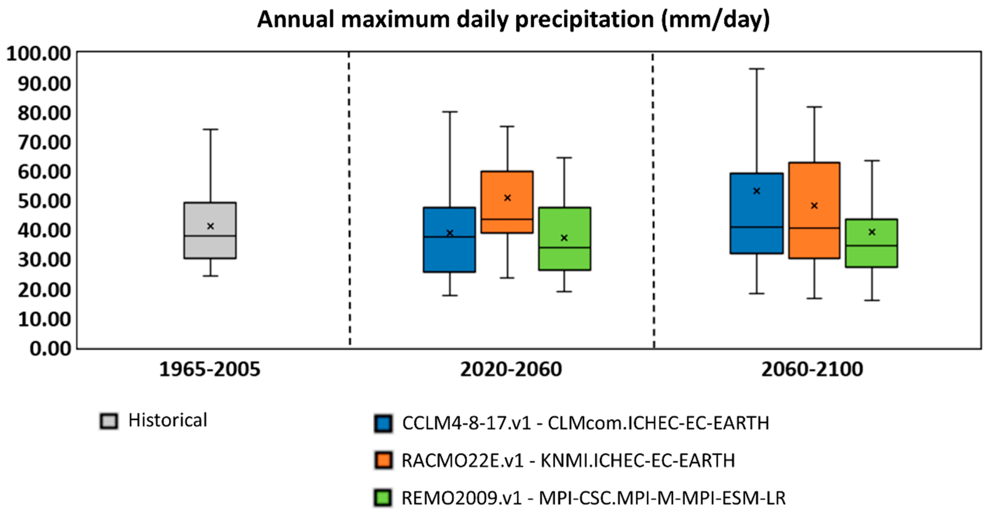
3.1. Projected Outcomes of Climate Models

The bias correction quantile mapping method was employed to correct inherent biases in raw precipitation outputs from RCMs, enhancing the reliability and accuracy of the projected data. By adjusting the cumulative distribution of modeled precipitation to better align with measured values, this approach effectively mitigated systematic discrepancies. As a result, the corrected data exhibited improved representation of key daily precipitation statistics, including average monthly maximum and average precipitation, as well as its standard deviation. These improvements, as detailed in

Table 2. Measurements and raw and bias-corrected data for the historical reference period of 1965–2005.

	Daily Max.	Daily Avg.	St. Dev.
Measurements (1965–2005)	52.23	1.21	4.22
CCLM4-8-17.v1-CLMcom.ICHEC-EC-EARTH Raw climatic data (1965-2005)	74.73	1.46	4.61
CCLM4-8-17.v1-CLMcom.ICHEC-EC-EARTH Bias-corrected data (1965–2005)	62.14	1.22	4.03
RACMO22E.v1-KNMI.ICHEC-EC-EARTH Raw climatic data (1965–2005)	39.03	1.13	3.45
RACMO22E.v1-KNMI.ICHEC-EC-EARTH Bias-corrected data (1965–2005)	50.29	1.22	4.16
REMO2009.v1-MPI-CSC.MPI-M-MPI-ESM-LR Raw climatic data (1965–2005)	59.58	1.42	4.52
REMO2009.v1-MPI-CSC.MPI-M-MPI-ESM-LR Bias-corrected data (1965–2005)	55.53	1.22	4.15

, demonstrate the effectiveness of the BCQM method in refining precipitation projections.

Table 3. Historical precipitation data and future projections based on the CCLM4-8-17.v1-CLMcom.ICHEC-EC-EARTH climate model.

	Measurements (mm/day) (1965–2005)				Downscaled Climatic Data (mm/day) (2020–2060)				Downscaled Climatic Data (mm/day) (2060–2100)
	Daily Min.	Daily Max.	Daily Avg.	St. Dev.	Daily Min.	Daily Max.	Daily Avg.	St. Dev.	Daily Min.	Daily Max.	Daily Avg.	St. Dev.
Oct.	0.00	62.70	1.31	4.68	0.00	66.28	1.20	4.51	0.00	87.92	1.21	5.09
Nov.	0.00	98.00	1.72	5.96	0.00	66.07	2.02	6.60	0.00	88.06	2.39	8.06
Dec.	0.00	54.50	1.62	4.80	0.00	35.69	1.31	2.80	0.00	22.86	1.63	2.93
Jan.	0.00	33.80	1.11	3.34	0.00	40.59	1.22	3.73	0.00	29.21	0.86	2.96
Feb.	0.00	49.20	1.22	3.88	0.00	46.24	1.11	3.48	0.00	33.76	0.89	2.70
Mar.	0.00	49.00	1.23	3.82	0.00	31.82	1.11	3.02	0.00	38.83	1.26	3.71
Apr.	0.00	54.20	1.25	3.85	0.00	35.74	1.16	3.43	0.00	34.90	0.85	3.01
May	0.00	38.10	1.53	4.32	0.00	51.25	1.56	3.91	0.00	86.33	1.67	4.89
June	0.00	39.60	0.89	3.47	0.00	63.64	1.06	4.19	0.00	109.21	1.11	4.78
July	0.00	60.70	0.92	4.37	0.00	49.77	1.03	4.18	0.00	155.29	0.86	5.48
Aug.	0.00	36.10	0.78	3.36	0.00	79.82	0.64	3.78	0.00	185.40	0.73	6.37
Sept.	0.00	50.90	0.93	3.93	0.00	56.68	0.92	3.47	0.00	53.08	0.73	3.30

,

Table 4. Historical precipitation data and future projections based on the RACMO22E.v1-KNMI.ICHEC-EC-EARTH climate model.

	Measurements (mm/day) (1965–2005)				Downscaled Climatic Data (mm/day) (2020–2060)				Downscaled Climatic Data (mm/day) (2060–2100)
	Daily Min.	Daily Max.	Daily Avg.	St. Dev.	Daily Min.	Daily Max.	Daily Avg.	St. Dev.	Daily Min.	Daily Max.	Daily Avg.	St. Dev.
Oct.	0.00	62.70	1.31	4.68	0.00	68.74	1.32	5.19	0.00	60.94	1.06	4.09
Nov.	0.00	98.00	1.72	5.96	0.00	105.42	2.51	8.75	0.00	79.22	2.33	8.18
Dec.	0.00	54.50	1.62	4.80	0.00	41.35	1.31	4.12	0.00	74.02	1.97	5.66
Jan.	0.00	33.80	1.11	3.34	0.00	28.49	1.04	2.56	0.00	19.63	0.74	2.07
Feb.	0.00	49.20	1.22	3.88	0.00	45.52	1.67	4.81	0.00	45.84	1.38	4.30
Mar.	0.00	49.00	1.23	3.82	0.00	92.80	1.56	4.88	0.00	45.06	1.48	4.49
Apr.	0.00	54.20	1.25	3.85	0.00	41.94	1.10	3.23	0.00	46.96	1.18	3.92
May	0.00	38.10	1.53	4.32	0.00	72.92	2.00	5.45	0.00	70.56	1.89	5.74
June	0.00	39.60	0.89	3.47	0.00	38.82	0.99	3.21	0.00	55.75	1.08	3.92
July	0.00	60.70	0.92	4.37	0.00	49.77	1.03	4.18	0.00	155.29	0.86	5.48
Aug.	0.00	36.10	0.78	3.36	0.00	30.92	0.53	2.09	0.00	29.74	0.79	2.75
Sept.	0.00	50.90	0.93	3.93	0.00	100.90	1.26	5.54	0.00	81.47	1.09	4.71

and

Table 5. Historical precipitation data and future projections based on the REMO2009.v1-MPI-CSC.MPI-M-MPI-ESM-LR climate model.

	Measurements (mm/day) (1965–2005)				Downscaled Climatic Data (mm/day) (2020–2060)				Downscaled Climatic Data (mm/day) (2060–2100)
	Daily Min.	Daily Max.	Daily Avg.	St. Dev.	Daily Min.	Daily Max.	Daily Avg.	St. Dev.	Daily Min.	Daily Max.	Daily Avg.	St. Dev.
Oct.	0.00	62.70	1.31	4.68	0.00	49.09	1.29	4.15	0.00	36.25	1.18	3.47
Nov.	0.00	98.00	1.72	5.96	0.00	64.50	1.90	6.11	0.00	63.37	2.01	6.15
Dec.	0.00	54.50	1.62	4.80	0.00	54.92	1.87	5.43	0.00	56.46	1.54	4.93
Jan.	0.00	33.80	1.11	3.34	0.00	31.16	1.21	3.36	0.00	40.98	1.22	3.60
Feb.	0.00	49.20	1.22	3.88	0.00	59.89	1.24	3.91	0.00	55.69	1.39	4.51
Mar.	0.00	49.00	1.23	3.82	0.00	52.69	1.51	4.55	0.00	29.66	1.05	3.11
Apr.	0.00	54.20	1.25	3.85	0.00	38.33	1.29	3.67	0.00	39.17	1.32	3.90
May	0.00	38.10	1.53	4.32	0.00	32.42	1.18	3.13	0.00	31.66	0.88	2.50
June	0.00	39.60	0.89	3.47	0.00	27.13	0.52	1.92	0.00	146.11	0.70	4.68
July	0.00	60.70	0.92	4.37	0.00	52.09	0.53	2.94	0.00	61.20	0.40	2.73
Aug.	0.00	36.10	0.78	3.36	0.00	49.81	0.61	2.83	0.00	50.13	0.52	2.55
Sept.	0.00	50.90	0.93	3.93	0.00	28.59	0.80	3.10	0.00	42.30	0.59	2.77

provide a comprehensive overview of daily precipitation statistics, presenting the minimum, maximum, and average values, along with the corresponding standard deviation, for each month across three distinct time periods: 1965–2005, 2020–2060, and 2060–2100. The findings highlight the variability and potential changes in precipitation dynamics across different temporal scales, revealing notable differences between climate models and the uncertainties associated with future projections. These variations underscore the complexities of predicting long-term precipitation trends and emphasize the importance of integrating both variability and uncertainty into climate adaptation strategies.

The analysis of annual maximum daily precipitation reveals significant variability in its temporal distribution across the three climate models, as shown in Figure 3. These variations highlight the distinct responses of each climate model to the projected climatic conditions under the RCP4.5 scenario.

For the historical period (1965–2005), the average annual maximum daily precipitation was estimated at 41.04 mm/day, serving as the baseline for comparison. Projections for the short-term future period (2020–2060) indicate that the average annual maximum daily precipitation is expected to decrease to 38.71 mm/day (a reduction of −5.68%) according to the CCLM4-8-17.v1-CLMcom.ICHEC-EC-EARTH model. In contrast, an increase to 50.61 mm/day (a rise of +23.32%) is projected by the RACMO22E.v1-KNMI.ICHEC-EC-EARTH model, while the REMO2009.v1-MPI-CSC.MPI-M-MPI-ESM-LR model forecasts a decline to 37.33 mm/day (a reduction of −9.04%).

In the long-term future period (2060–2100), the projected trends also exhibit notable differences among the models. The CCLM4-8-17.v1-CLMcom.ICHEC-EC-EARTH model projects a substantial increase in the average annual maximum daily precipitation to 52.95 mm/day, representing a +29.02% change relative to the historical baseline. Similarly, the RACMO22E.v1-KNMI.ICHEC-EC-EARTH model predicts an elevated value of 48.16 mm/day, corresponding to a +17.35% increase. Conversely, the REMO2009.v1-MPI-CSC.MPI-M-MPI-ESM-LR model estimates a moderate increase to 39.02 mm/day, equating to a −4.92% change compared to the historical period.

Furthermore, as illustrated in Figure 3, the annual maximum daily precipitation consistently exhibits average values that are higher than their respective medians. This characteristic underscore the right skewness of the precipitation dataset, a statistical trait that reflects the occurrence of infrequent and intense precipitation events that significantly influence the mean. Right-skewed distributions are a well-documented feature of precipitation datasets, particularly in regions subject to pronounced seasonal variability or periodic extreme weather phenomena. This skewness is indicative of a climate regime where extreme events dominate precipitation trends, and it has important implications for hydrological modeling and risk assessments.

Further analysis of the box plots presented in Figure 3 reveals notable differences between the historical and future periods. Specifically, the whiskers of the box plots for the future periods (2020–2060 and 2060–2100) concerning the CCLM4-8-17.v1-CLMcom.ICHEC-EC-EARTH model are significantly longer than those observed for the historical baseline (1965–2005). This observation suggests a wider range of variability in annual maximum daily precipitation in the future, indicating the potential for more extreme values. The lengthened whiskers in the future projections highlight the increased likelihood of extremely high values, emphasizing the importance of accounting for climate extremes in future planning scenarios. This is particularly relevant for infrastructure design and flood risk assessments, where planning for variability and uncertainty is critical.

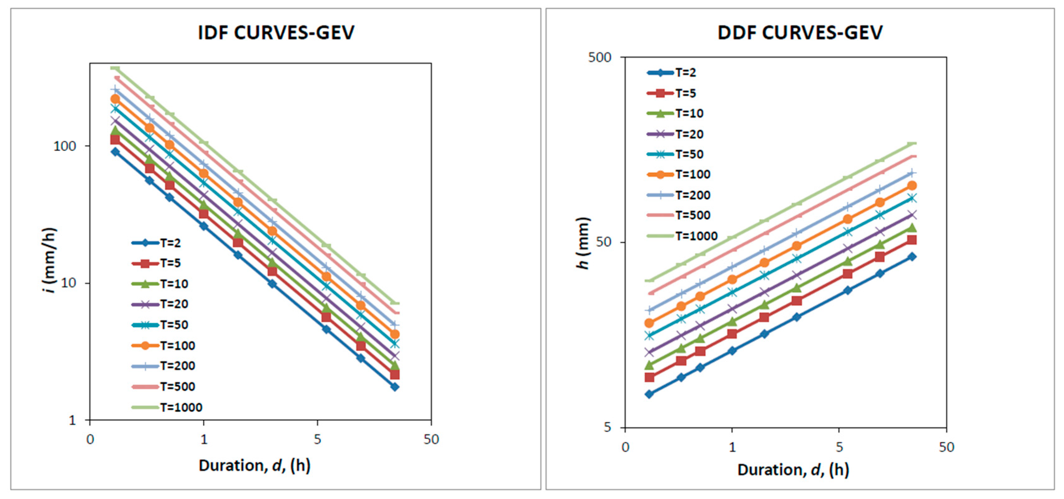
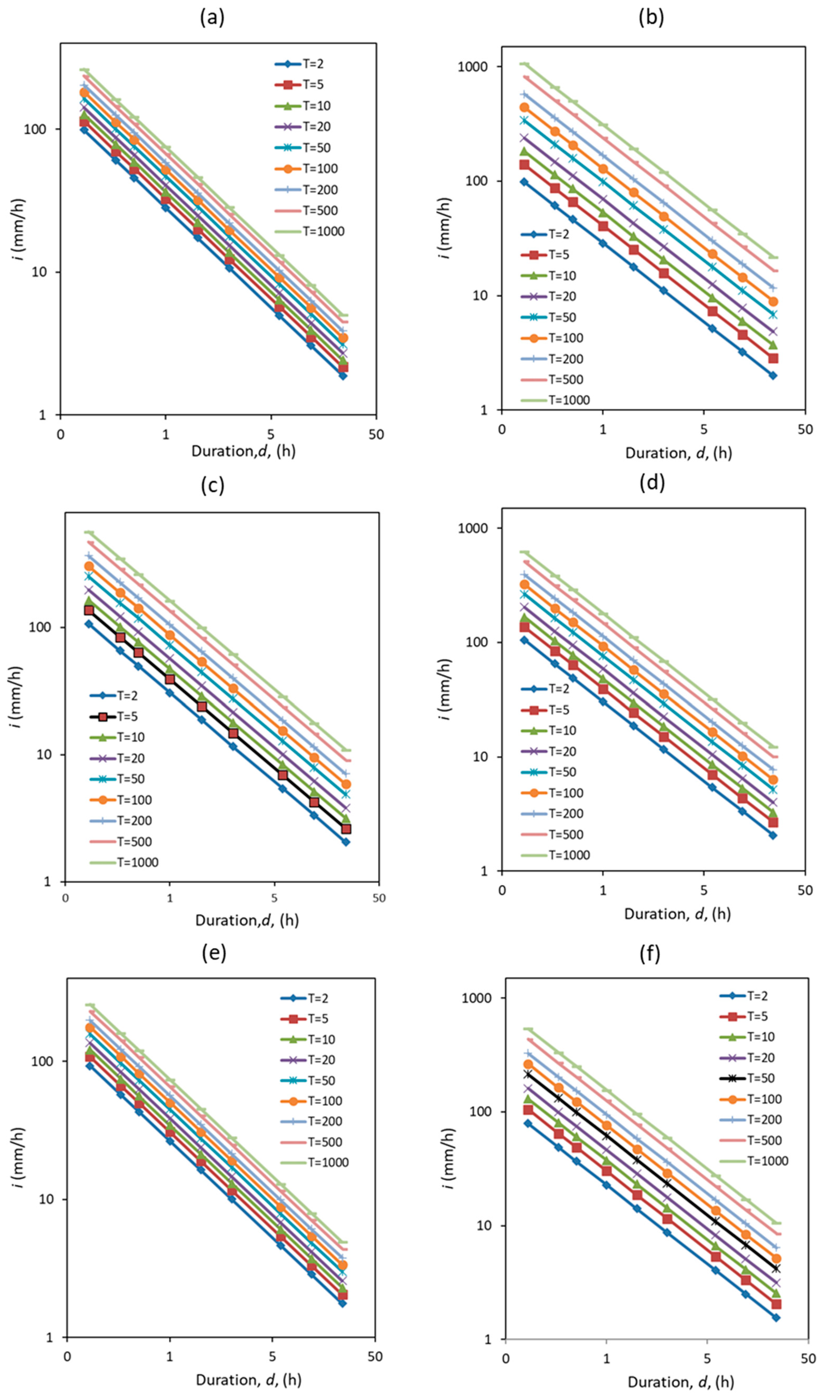
3.2. Development of IDF Curves

The scaling behavior of rainfall extremes in the study area is assessed using available annual maximum rainfall data at the Thessaloniki airport (station Mikra) provided by the HNMS covering a period of 25 years (1963–1987), corresponding to durations of 5 min, 10 min, 15 min, 30 min, 1 h, 2 h, 3 h, 6 h, 12 h, and 24 h. The L-moment approach is initially used to assess the GEV parameters for all rainfall durations of the available fine-scale dataset. Equation (6) is then used to assess the three NCMs for all rainfall durations, and a logarithmic plot of the first three NCMs of rainfall at the Thessaloniki station with rainfall duration is then constructed (Figure 4). Figure 4 also includes the power laws (Equation (9)) resulting for all three NCMs.

The log linearity of the GEV NCMs of annual maximum rainfall is illustrated in the plot, indicating the power law dependency (i.e., scaling) of the statistical moments with duration (Equations (9) and (11)). The slopes in the plot are proportional to the scaling exponent β. Two different scaling regimes are evident from Figure 4, one in the 5 min to 30 min interval and one in the 30 min to 24 h interval, indicating a difference in extreme rainfall dynamic at the finest temporal scales. This difference is confirmed through the linearity of the scaling exponent β(k) with moment order, k, as shown in Figure 5a,b for the intervals of [5, 30] min and [0.5, 24] h.

After assessing the relationships of GEV NCMs with extreme rainfall duration, the three NCMs of the daily rainfall predictions are used in combination with the scaling exponent β(k), which is kept constant for all time intervals and climate realizations, to assess the coefficient a(k) (see Equation (9)) of the annual maximum precipitation process. The coefficient can be used to determine the newly defined NCMs m_k for each sub-daily rainfall duration (using Equation (9)). The three GEV NCMs for each rainfall duration are then utilized to assess the respective GEV parameters by means of Equation (6). After assessing the GEV parameters for all rainfall durations and for all 40-year intervals considered, the extreme quantiles (return levels) corresponding to return periods of 2, 5, 10, 20, 50, 100, 200, 500, and 1000 years are estimated using Equation (4). IDF and DDF curves are then created for all 40-year periods considered (historical and future periods from RCMs) based on Equation (13). Figure 6 presents the IDF and DDF curves in Thessaloniki, Greece, for the historical/reference climate period (1965–2005). Figure 7 presents the IDF curves for all climate models considered in this work (CCLM, RACMO, and REMO) and for both future periods, namely 2020–2060 and 2060–2100.

Table 6. IDF and DDF curve equations for the historical and future climates in Thessaloniki, Greece.

Climate Period and RCM	DDF Equation	IDF Equation
1965–2005 Historical/Reference	33.19T0.227d0.302	33.19T0.227d−0.698
2020–2060 CCLM	28.83T0.157d0.300	28.83T0.157d−0.700
2020–2060 RACMO	44.70T0.268d0.303	44.70T0.268d−0.697
2020–2060 REMO	27.73T0.165d0.300	27.73T0.165d−0.700
2060–2100 CCLM	61.24T0.383d0.311	61.24T0.383d−0.689
2060–2100 RACMO	47.13T0.287d0.306	47.13T0.287d−0.694
2060–2100 REMO	38.02T0.309d0.305	38.02T0.309d−0.695

presents the IDF and DDF curve equations (Equation (13)) for the historical/reference climate period (1965–2005), as well as for the two future periods (2020–2060 and 2060–2100) for all three RCMs studied in this work.

Rainfall extremes for the future period of 2020–2060 are assessed higher than those of the historical climate only for RACMO RCM. More specifically, 100-year rainfall events of 1 h duration are almost 39% higher than those of the historical climate. CCLM and REMO RCMs produce lower 100-year rainfall extremes (1 h duration) up to 17.3% and 20%, respectively. The future period of 2060–2100 appears more energetic with respect to extreme precipitation events, compared to the future period of 2020–2060. In the future period of 2060–2100, 100-year rainfall events of 1 h duration are almost 150%, 7%, and 51.5% higher than those of the future period of 2020–2060 for CCLM, RACMO, and REMO RCM, respectively.

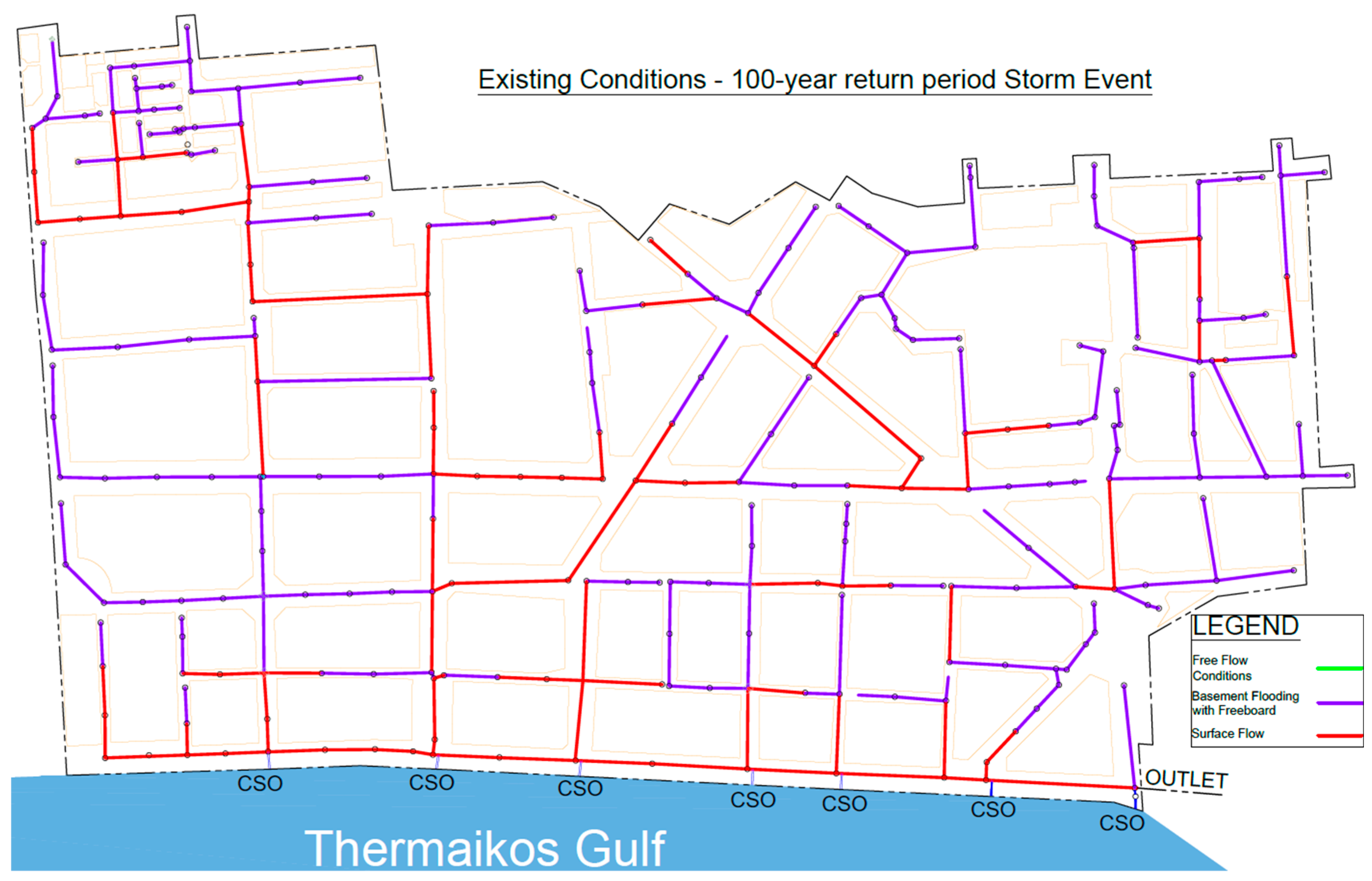
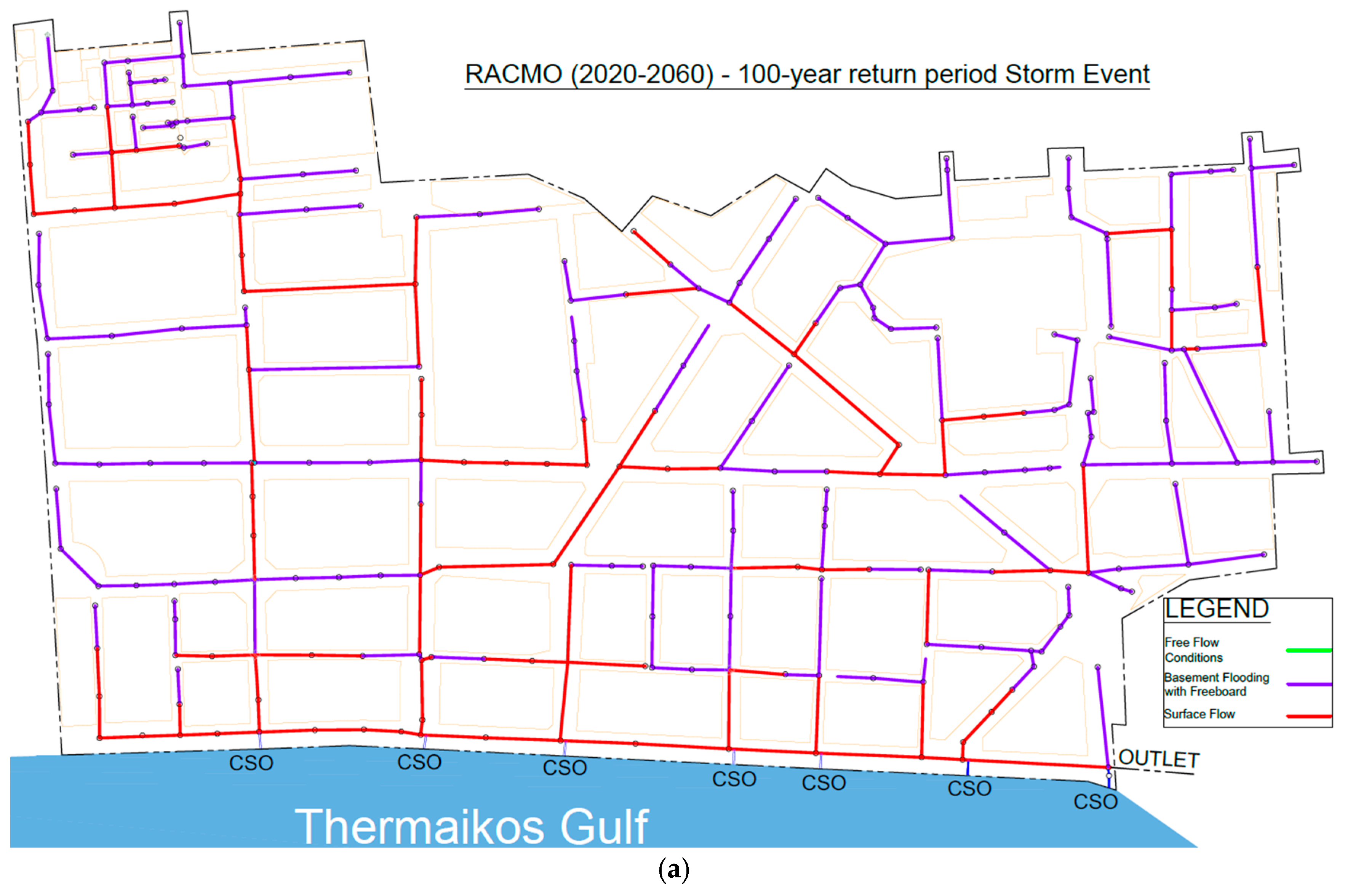
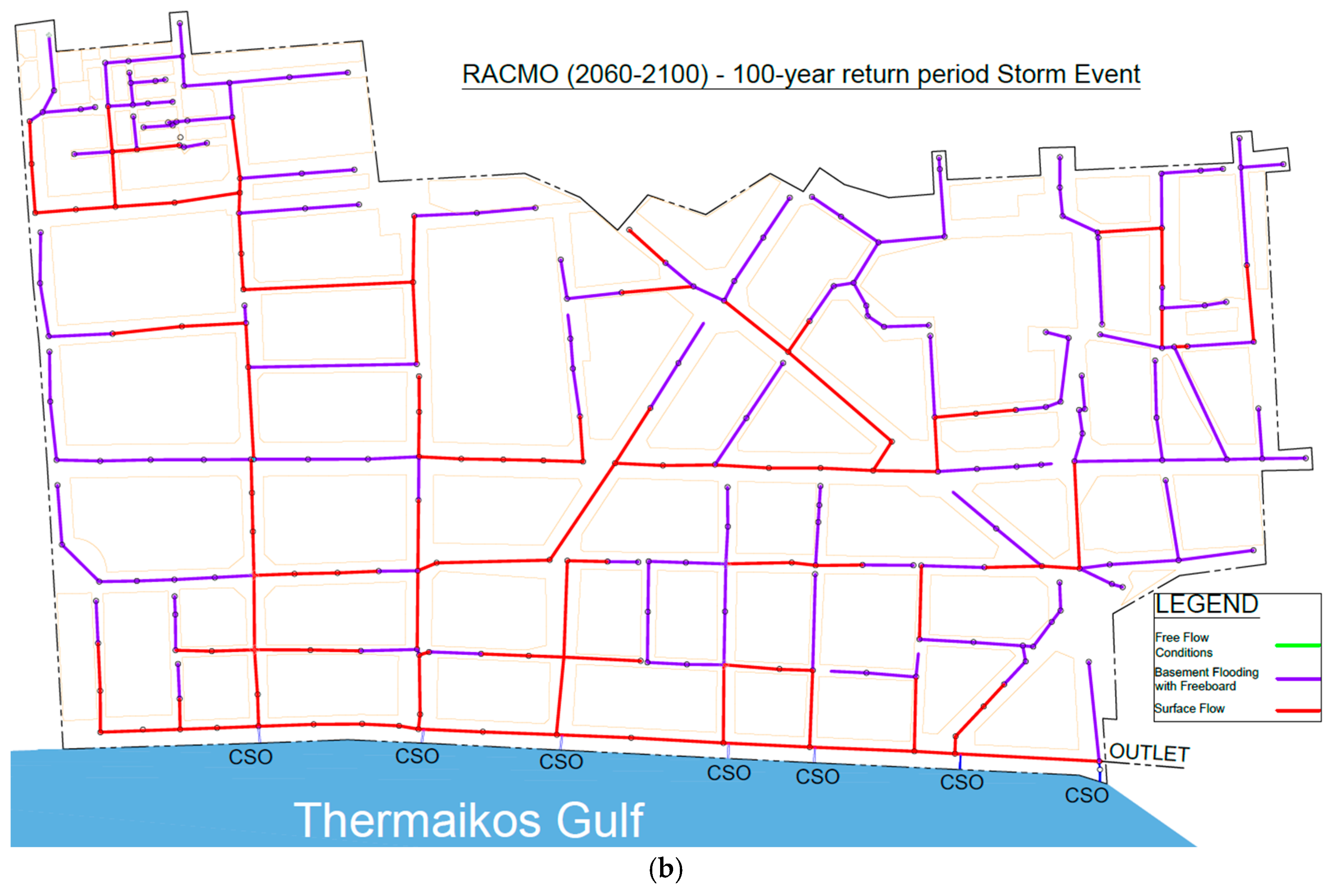
3.3. Hydraulic Results

The storm rainfall events analyzed in this research were obtained from the IDF relationships established in Section 3.2. Rainfall events for various return periods with a 1 h duration were generated; however, the model was assessed exclusively for the 100-year return period, as it represents the worst-case scenario. The model that was calibrated and validated by Galiatsatou et al. [42] is also employed in this study. More specifically, since flow monitoring data were unavailable for the center of Thessaloniki, the calibration of the model was conducted through a qualitative approach. For the dry weather calibration, the focus was on adjusting the population density, baseflow, and diurnal pattern factor. For the wet weather calibration, historical rainfall events known to cause flooding were utilized as valuable data to refine the model for low-frequency return events. This step was critical to ensure the model’s reliability in predicting flooding in areas with past flooding records. Three major past events were selected for this purpose: (a) 11 May 2018, (b) 17 June 2023, and (c) 9 May 2024. These events were used to adjust parameters related to the RTK hydrograph, infiltration rates, initial loss, direct runoff coefficients, and runoff routing for both impervious and pervious surfaces.

Figure 8 illustrates the hydraulic results for current conditions under the worst-case scenario of a 100-year return period storm event. Meanwhile, Figure 9, Figure 10 and Figure 11 show the results derived from rainfall distributions based on the CCLM, RACMO, and REMO, respectively, for the periods of 2020–2060 and 2060–2100. Flooding correlation is assessed by examining conduit surcharge conditions and the hydraulic grade line (HGL) at nodes relative to a predefined theoretical basement elevation of 2 m below ground level. Manholes are depicted by black dots, and dark blue lines along the coastline represent CSO locations within the network. Sewer segments are color-coded as follows: green for segments where the HGL is more than 2 m below ground level, purple for those experiencing basement flooding (where the HGL is less than 2 m from the surface but remains underground), and red for areas where surface runoff occurs. Some of the pipes do not have an upstream node, and catch basins are directly connected to them. As a result, these pipes are simulated using only fictitious nodes, which are not represented in the color-coded figures. For simplicity, results for events with a return period of less than 100 years are not presented, as the issue is more effectively highlighted under the worst-case scenario.

Table 7. Combined sewer system performance under historical and future climates in Thessaloniki, Greece.

Scenario (100-Year Return Period)	Combined Sewer Overflow Volume (m3)
Existing Conditions	12,273
2020–2060 CCLM	10,735
2020–2060 RACMO	17,117
2020–2060 REMO	10,012
2060–2100 CCLM	25,514
2060–2100 RACMO	18,605
2060–2100 REMO	15,799

provides a summary of the simulation results and the impact of future climate projections on combined sewer overflow volumes (CSO volumes).

As shown in Figure 8, Figure 9, Figure 10 and Figure 11 and Table 7, in the near-term period from 2020 to 2060, the projected CSO volumes vary significantly across the models. The CCLM (10,735 m³) and REMO (10,012 m³) predict lower overflow volumes compared to the existing conditions (12,273 m³), suggesting that these models anticipate either a decrease in extreme rainfall intensity or a redistribution of rainfall events. However, the RACMO (17,117 m³) shows an increase in CSO volumes, indicating a potential rise in extreme precipitation events under this scenario. For the long-term period from 2060 to 2100, all models predict an increase in CSO volumes compared to existing conditions, highlighting a worsening overflow problem in the future. Among them, CCLM (25,514 m³) projects the highest overflow volume, which is more than doubling the existing conditions. This suggests that under this scenario, intense rainfall events will become significantly more frequent or severe, putting additional stress on urban drainage systems. The RACMO (18,605 m³) also indicates a continuous increase in CSO volumes, though at a lower magnitude than CCLM, while REMO (15,799 m³) suggests a moderate increase over time. These projections carry important implications for future flood management strategies. The substantial increase in overflow volumes predicted by the CCLM indicates that the most robust adaptation measures may be necessary in this scenario. These could include significant infrastructure enhancements such as increasing storage capacity, upgrading conveyance systems, and implementing nature-based solutions like green infrastructure. The variations among the models highlight the uncertainty in climate projections, underscoring the need for adaptable and flexible flood management strategies capable of addressing a broad spectrum of potential future conditions.

For short-term flood risk management, the RACMO is the most suitable as it predicts an increase in CSO volumes due to more extreme rainfall events between 2020 and 2060. For long-term planning, the CCLM should be prioritized, as it projects the most significant increase in CSO volumes, suggesting a future with more intense rainfall and greater pressure on urban drainage systems. The REMO provides a moderate scenario and is useful for balancing future projections, offering a more conservative approach for overall flood risk management.

4. Conclusions

This study underscores the profound impact of climate change on combined sewer overflows within the Thessaloniki City Center network. Detailed analysis of current and projected intensity–duration–frequency (IDF) curves, derived from the CCLM, RACMO, and REMO, indicates that the drainage system is poised to face significant challenges as rainfall intensities increase. Modeling conducted with InfoWorks further reveals that the anticipated escalation in rainfall intensity may overwhelm the system’s capacity to manage peak flows, thereby elevating the risk of flooding and increasing overflow volumes.

For the near-term projections, the key findings indicate that the CCLM projects combined sewer overflow (CSO) volumes of 10,735 m³, which is lower than the current volume of 12,273 m³. The REMO predicts a similar trend, forecasting CSO volumes at 10,012 m³. However, the RACMO contrasts with the other two by predicting an increase to 17,117 m³, suggesting that more frequent or intense extreme precipitation events may occur. These divergent outcomes highlight the uncertainty in short-term climate projections and emphasize the importance of conducting multi-model assessments.

For the long-term projections, all models agree on an increase in CSO volumes compared to current conditions. The CCLM shows the most dramatic increase, forecasting an overflow volume of 25,514 m³,which is more than double the current volume. The RACMO indicates a moderate increase to 18,605 m³, while the REMO projects a moderate rise to 15,799 m³. Despite the varying magnitudes of the increases, the consistent upward trend in all models clearly points to a worsening overflow problem, with urban drainage systems likely to face substantial additional stress in the future.

Considering these findings, it is imperative to consider a range of mitigation strategies. These include separating stormwater from sanitary flows to reduce the system’s load, disconnecting downspouts to limit direct contributions to overflows, and implementing nature-based solutions, such as green roofs and permeable pavements, to enhance overall system resilience. Such measures are vital for reducing flood risks and ensuring long-term urban sustainability amidst evolving climatic conditions. Moreover, future research will be dedicated to exploring additional capacity enhancement strategies, including the integration of offline storage and low-impact development techniques, to further bolster the system’s adaptability in the face of continued climate change.

References

1. Colmet-Daage, A.; Sanchez-Gomez, E.; Ricci, S.; Llovel, C.; Borrell Estupina, V.; Quintana-Seguí, P.; Llasat, M.C.; Servat, E. Evaluation of uncertainties in mean and extreme precipitation under climate change for northwestern Mediterranean watersheds from high-resolution Med and Euro-CORDEX ensembles. Hydrol. Earth Syst. Sci. 2018, 22, 673–687. [Google Scholar] [CrossRef]
2. Tramblay, Y.; Somot, S. Future evolution of extreme precipitation in the Mediterranean. Clim. Change 2018, 151, 289–302. [Google Scholar] [CrossRef]
3. Berg, P.; Christensen, O.B.; Klehmet, K.; Lenderink, G.; Olsson, J.; Teichmann, C.; Yang, W. Summertime precipitation extremes in a EURO-CORDEX 0.11° ensemble at an hourly resolution. Nat. Hazards Earth Syst. Sci. 2019, 19, 957–971. [Google Scholar] [CrossRef]
4. Cardell, M.F.; Amengual, A.; Romero, R.; Ramis, C. Future extremes of temperature and precipitation in Europe derived from a combination of dynamical and statistical approaches. Int. J. Climatol. 2020, 40, 4800–4827. [Google Scholar] [CrossRef]
5. Di Sante, F.; Coppola, E.; Giorgi, F. Projections of river floods in Europe using EURO-CORDEX, CMIP5 and CMIP6 simulations. Int. J. Climatol. 2021, 41, 3203–3221. [Google Scholar] [CrossRef]
6. Ivušić, S.; Güttler, I.; Horvath, K. Overview of mean and extreme precipitation climate changes across the Dinaric Alps in the latest EURO-CORDEX ensemble. Clim. Dyn. 2024, 62, 10785–10815. [Google Scholar] [CrossRef]
7. Vautard, R.; Kadygrov, N.; Iles, C.; Boberg, F.; Buonomo, E.; Bülow, K.; Coppola, E.; Corre, L.; van Meijgaard, E.; Nogherotto, R.; et al. Evaluation of the Large EURO-CORDEX Regional Climate Model Ensemble. JGR Atmos. 2021, 126, e2019JD032344. [Google Scholar] [CrossRef]
8. Boe, J.; Mass, A.; Deman, J. A simple hybrid statistical–dynamical downscaling method for emulating regional climate models over Western Europe. Evaluation, application, and role of added value? Clim. Dyn. 2022, 61, 271–294. [Google Scholar] [CrossRef]
9. Ascenso, A.; Augusto, B.; Coelho, S.; Menezes, I.; Monteiro, A.; Rafael, S.; Ferreira, J.; Gama, C.; Roebeling, P.; Miranda, A.I. Assessing Climate Change Projections through High-Resolution Modelling: A Comparative Study of Three European Cities. Sustainability 2024, 16, 7276. [Google Scholar] [CrossRef]
10. Cox, P.; Stephenson, D. Climate change—A changing climate for prediction. Science 2007, 317, 207–208. [Google Scholar] [CrossRef]
11. Déqué, M.; Rowell, D.P.; Lüthi, D.; Giorgi, F.; Christensen, J.H.; Rockel, B.; Jacob, D.; Kjellström, E.; de Castro, M.; van den Hurk, B. An intercomparison of regional climate simulations for Europe: Assessing uncertainties in model projections. Clim. Change 2007, 81, 53–70. [Google Scholar] [CrossRef]
12. Elía, R.; Caya, D.; Côté, H.; Frigon, A.; Biner, S.; Giguère, M.; Paquin, D.; Harvey, R.; Plummer, D. Evaluation of uncertanties in the CRCM-simulated North American climate. Clim. Dyn. 2008, 30, 113–132. [Google Scholar] [CrossRef]
13. Kendon, E.J.; Rowell, D.P.; Jones, R.G.; Buonomo, E. Robustness of future changes in local precipitation extremes. J. Clim. 2008, 21, 4280–4297. [Google Scholar] [CrossRef]
14. Gogien, F.; Dechesne, M.; Martinerie, R.; Lipeme Kouyi, G. Assessing the impact of climate change on Combined Sewer Overflows based on small time step future rainfall timeseries and long-term continuous sewer network modelling. Water Res. 2023, 230, 119504. [Google Scholar] [CrossRef]
15. Zhang, H.; Yang, Z.; Cai, Y.; Qiu, J.; Huang, B. Impacts of Climate Change on Urban Drainage Systems by Future Short-Duration Design Rainstorms. Water 2021, 13, 2718. [Google Scholar] [CrossRef]
16. Willems, P.; Olsson, J.; Arnbjerg-Nielsen, K.; Beecham, S.; Pathirana, A.; Gregersen, I.B.; Madsen, H.; Nguyen, V.-T.-V. Impacts of Climate Change on Rainfall Extremes and Urban Drainage; IWA Publishing: London, UK, 2012. [Google Scholar]
17. Haerter, J.O.; Hagemann, S.; Moseley, C.; Piani, C. Climate model bias correction and the role of timescales. Hydrol. Earth Syst. Sci. 2011, 15, 1065–1079. [Google Scholar] [CrossRef]
18. Themeɮl, M.J.; Gobiet, A.; Heinrich, G. Empirical statistical downscaling and error correction of regional climate models and its impact on the climate change signal. Clim. Change 2012, 112, 449–468. [Google Scholar]
19. Heo, J.H.; Ahn, H.; Shin, J.Y.; Kjeldsen, T.R.; Jeong, C. Probability distributions for a quantile mapping technique for a bias correction of precipitation data: A case study to precipitation data under climate change. Water 2019, 11, 1475. [Google Scholar] [CrossRef]
20. Tani, S.; Gobiet, A. Quantile mapping for improving precipitation extremes from regional climate models. J. Agrometeorol. 2019, 21, 434–443. [Google Scholar] [CrossRef]
21. Holthuijzen, M.; Beckage, B.; Clemins, P.J.; Higdon, D.; Winter, J.M. Robust bias-correction of precipitation extremes using a novel hybrid empirical quantile-mapping method: Advantages of a linear correction for extremes. Theor. Appl. Climatol. 2022, 149, 863–882. [Google Scholar] [CrossRef]
22. Gudmundsson, L.; Bremnes, J.B.; Haugen, J.E.; Engen-Skaugen, T. Technical Note: Downscaling RCM precipitation to the station scale using statistical transformations–a comparison of methods. Hydrol. Earth Syst. Sci. 2012, 16, 3383–3390. [Google Scholar] [CrossRef]
23. Teutschbein, C.; Seibert, J. Bias correction of regional climate model simulations for hydrological climate-change impact studies: Review and evaluation of different methods. J. Hydrol. 2012, 16, 12–29. [Google Scholar] [CrossRef]
24. Chandra, R.R.; Papalexiou, S.M. Precipitation Bias Correction: A Novel Semi-parametric Quantile Mapping Method. Earth Space Sci. 2023, 10, e2023EA002823. [Google Scholar]
25. Nguyen, V.-T.-V.; Nguyen, T.-D.; Ashkar, F. Regional Frequency Analysis of Extreme Rainfalls. Water Sci. Technol. 2002, 45, 75–81. [Google Scholar] [CrossRef]
26. Terti, G.; Galiatsatou, P.; Prinos, P. Effects of climate change on the estimation of intensity-duration-frequency (IDF) curves for Thessaloniki, Greece. In Proceedings of the 9th International Conference on Urban Drainage Modelling, Belgrade, Serbia, 3–7 September 2012. [Google Scholar]
27. Ghanmi, H.; Bargaoui, Z.; Mallet, C. Estimation of intensity-duration-frequency relationships according to the property of scale invariance and regionalization analysis in a Mediterranean coastal area. J. Hydrol. 2016, 541, 38–49. [Google Scholar] [CrossRef]
28. Yeo, M.H.; Nguyen, V.T.V.; Kpodonu, T.A. Characterizing extreme rainfalls and constructing confidence intervals for IDF curves using Scaling-GEV distribution model. Int. J. Climatol. 2021, 41, 456–468. [Google Scholar] [CrossRef]
29. Galiatsatou, P.; Iliadis, C. Intensity-Duration-Frequency Curves at Ungauged Sites in a Changing Climate for Sustainable Stormwater Networks. Sustainability 2022, 14, 1229. [Google Scholar] [CrossRef]
30. Iliadis, C.; Galiatsatou, P.; Glenis, V.; Prinos, P.; Kilsby, C. Urban flood modelling under extreme rainfall conditions for building-level flood exposure analysis. Hydrology 2023, 10, 172. [Google Scholar] [CrossRef]
31. Koutsoyiannis, D.; Kozonis, D.; Manetas, A. A mathematical framework for studying rainfall intensity-duration-frequency relationships. J. Hydrol. 1998, 206, 118–135. [Google Scholar] [CrossRef]
32. Veneziano, D.; Furcolo, P. Multifractality of rainfall and scaling of intensity-duration-frequency curves. Water Resour. Res. 2002, 38, 42-1–42-12. [Google Scholar] [CrossRef]
33. Singh, V.P.; Zhang, L. IDF curves using the Frank Archimedean copula. J. Hydrol. Eng. 2007, 12, 651–662. [Google Scholar] [CrossRef]
34. Salas, J.D.; Obeysekera, J. Revisiting the concepts of return period and risk for nonstationary hydrologic extreme events. J. Hydrol. Eng. 2014, 19, 554–568. [Google Scholar] [CrossRef]
35. Salas, J.D.; Obeysekera, J.; Vogel, R.M. Techniques for assessing water infrastructure for nonstationary extreme events: A review. Hydrol. Sci. J. 2018, 63, 325–352. [Google Scholar] [CrossRef]
36. Yan, L.; Xiong, L.; Jiang, C.; Zhang, M.; Wang, D.; Xu, C.Y. Updating intensity–duration–frequency curves for urban infrastructure design under a changing environment. Wiley Interdiscip. Rev. Water 2021, 8, e1519. [Google Scholar] [CrossRef]
37. Martel, J.L.; Mailhot, A.; Brissette, F.; Caya, D. Role of natural climate variability in the detection of anthropogenic climate change signal for mean and extreme precipitation at local and regional scales. J. Clim. 2018, 31, 4241–4263. [Google Scholar] [CrossRef]
38. Schlef, K.E.; Kunkel, K.E.; Brown, C.; Demissie, Y.; Lettenmaier, D.P.; Wagner, A.; Yan, E. Incorporating non-stationarity from climate change into rainfall frequency and intensity-duration-frequency (IDF) curves. J. Hydrol. 2023, 616, 128757. [Google Scholar] [CrossRef]
39. Serinaldi, F.; Kilsby, C.G. Stationarity is undead: Uncertainty dominates the distribution of extremes. Adv. Water Resour. 2015, 77, 17–36. [Google Scholar] [CrossRef]
40. Serinaldi, F.; Kilsby, C.G.; Lombardo, F. Untenable nonstationarity: An assessment of the fitness for purpose of trend tests in hydrology. Adv. Water Resour. 2018, 111, 132–155. [Google Scholar] [CrossRef]
41. Kourtis, I.M.; Tsihrintzis, V.A. Adaptation of urban drainage networks to climate change: A review. Sci. Total Environ. 2021, 771, 145431. [Google Scholar] [CrossRef]
42. Galiatsatou, P.; Zafeirakou, A.; Nikoletos, I.; Gkatzioura, A.; Kapouniari, M.; Katsoulea, A.; Malamataris, D.; Kavouras, I. Capacity Assessment of a Combined Sewer Network under Different Weather Conditions: Using Nature-Based Solutions to Increase Resilience. Water 2024, 16, 2862. [Google Scholar] [CrossRef]
43. Al-Mukhtar, M.; Dunger, V.; Merkel, B. Runoff and sediment yield modeling by means of WEPP in the Bautzen dam catchment, Germany. Environ. Earth Sci. 2014, 72, 2051–2063. [Google Scholar] [CrossRef]
44. Nasiry, M.K.; Said, S.; Ansari, S.A. Analysis of surface runoff and sediment yield under simulated rainfall. Model. Earth Syst. Environ. 2023, 9, 157–173. [Google Scholar] [CrossRef]
45. Cojoc, L.; de Castro-Català, N.; de Guzmán, I.; González, J.; Arroita, M.; Besolí-Mestres, N.; Cadena, I.; Freixa, A.; Gutiérrez, O.; Larrañaga, A.; et al. Pollutants in urban runoff: Scientific evidence on toxicity and impacts on freshwater ecosystems. Chemosphere 2024, 369, 143806. [Google Scholar] [CrossRef] [PubMed]
46. Jacob, D.; Petersen, J.; Eggert, B.; Alias, A.; Christensen, O.B.; Bouwer, L.M.; Braun, A.; Colette, A.; Déqué, M.; Georgievski, G.; et al. EURO-CORDEX: New high-resolution climate change projections for European impact research. Reg. Environ. Change 2014, 14, 563–578. [Google Scholar] [CrossRef]
47. Galiatsatou, P.; Prinos, P. Joint probability analysis of extreme wave heights and storm surges in the Aegean Sea in a changing climate. E3S Web Conf. 2016, 7, 02002. [Google Scholar] [CrossRef]
48. Silva Lomba, J.; Fraga Alves, M.I. L-moments for automatic threshold selection in extreme value analysis. Stoch. Environ. Res. Risk Assess. 2020, 34, 465–491. [Google Scholar] [CrossRef]
49. Galiatsatou, P.; Prinos, P. Bivariate analysis of extreme wave and storm surge events. Determining the failure area of structures. Open Ocean Eng. J. 2011, 4, 3–14. [Google Scholar] [CrossRef]
50. Galiatsatou, P.; Prinos, P.; Sanchez-Arcilla, A. Estimation of extremes: Conventional versus Bayesian techniques. J. Hydraul. Res. 2008, 46, 211–223. [Google Scholar] [CrossRef]
51. Desramaut, N. Estimation of Intensity Duration Frequency Curves for Current and Future Climates. Master’s Thesis, McGill University, Montreal, QC, Canada, 2008; pp. 1–75. [Google Scholar]
52. InfoWorks ICM Help Documentation. Available online: https://help-innovyze.refined.site/space/infoworksicm/18219088/ (accessed on 31 May 2024).
53. Sheng, J.G.; Dan, Y.D.; Liu, C.S.; Ma, L.M. Study of Simulation in Storm Sewer System of Zhenjiang Urban by Infoworks ICM. Model. Appl. Mech. Mater. 2012, 193, 683–686. [Google Scholar] [CrossRef]
54. Peng, H.-Q.; Liu, Y.; Wang, H.-W.; Ma, L.-M. Assessment of the service performance of drainage system and transformation of pipeline network based on urban combined sewer system model. Environ. Sci. Pollut. Res. 2015, 22, 15712–15721. [Google Scholar] [CrossRef]
55. Biswas, R.R. Modelling seismic effects on a sewer network using Infoworks ICM. Indian J. Sci. Technol. 2017, 10, 1–9. [Google Scholar] [CrossRef]
56. Sidek, L.M.; Jaafar, A.S.; Majid, W.H.A.W.A.; Basri, H.; Marufuzzaman, M.; Fared, M.M.; Moon, W.C. High-resolution hydrological-hydraulic modeling of urban floods using InfoWorks ICM. Sustainability 2021, 13, 10259. [Google Scholar] [CrossRef]
57. Leitao, J.; Simoes, N.; Pina, R.D.; Ochoa-Rodriguez, S.; Onof, C.; Sa Marques, A. Stochastic evaluation of the impact of sewer inlets’ hydraulic capacity on urban pluvial flooding. Stoch. Environ. Res. Risk Assess. 2017, 31, 1907–1922. [Google Scholar] [CrossRef]
58. Cheng, T.; Xu, Z.; Hong, S.; Song, S. Flood risk zoning by using 2D hydrodynamic modeling: A case study in Jinan City. Math. Probl. Eng. 2017, 2017, 5659197. [Google Scholar] [CrossRef]
59. Wang, K.; Chen, J.; Hu, H.; Tang, Y.; Huang, J.; Wu, Y.; Lu, J.; Zhou, J. Urban Waterlogging Simulation and Disaster Risk Analysis Using InfoWorks Integrated Catchment Management: A Case Study from the Yushan Lake Area of Ma’anshan City in China. Water 2024, 16, 3383. [Google Scholar] [CrossRef]
60. Nikoletos, I.; Katsifarakis, K. The Method of Images Revisited: Approximate Solutions in Wedge-Shaped Aquifers of Arbitrary Angle. Water Resour. Res. 2024, 60, e2022WR034347. [Google Scholar] [CrossRef]
61. Jin, X.; Mu, Y. Hydrodynamic Simulation of Urban Waterlogging Based on an Improved Vertical Flow Exchange Method. Water 2024, 16, 1563. [Google Scholar] [CrossRef]
Figure 1. Drainage area of Thessaloniki’s city center network coordinates 40.6323° N, 22.9459° E, EPSG: 32634-WGS 84/UTM zone 34° N.
Climate 13 00082 g001
Figure 2. Schematic diagram of the pipe network in the city center of Thessaloniki.
Climate 13 00082 g002
Figure 3. Box–and–whisker diagrams of annual maximum daily precipitation for the three climate models in the study area.
Climate 13 00082 g003
Figure 4. The log–log plot of GEV NCMs of annual maximum rainfall versus duration at Mikra station, Thessaloniki.
Climate 13 00082 g004
Figure 5. The scaling exponent β(k) versus the GEV NCM order for the following intervals: (a) 5 min to 30 min and (b) 30 min to 1 h.
Climate 13 00082 g005
Figure 6. IDF and DDF curves for the historical/reference period (1965–2005) in Thessaloniki, Greece.
Climate 13 00082 g006
Figure 7. IDF curves for the future climate in Thessaloniki, Greece: (a) 2020–2060 with CCLM RCM, (b) 2060–2100 with CCLM RCM, (c) 2020–2060 with RACMO RCM, (d) 2060–2100 with RACMO RCM, (e) 2020–2060 with REMO RCM, and (f) 2060–2100 with REMO RCM.
Climate 13 00082 g007
Figure 8. Hydraulic results for existing conditions under a 100-year return period.
Climate 13 00082 g008
Figure 9. Hydraulic results using the rainfall distribution derived from CCLM for a 100 year return period during (a) 2020–2060 and (b) 2060–2100.
Climate 13 00082 g009aClimate 13 00082 g009b
Figure 10. Hydraulic results using the rainfall distribution derived from RACMO for a 100-year return period during (a) 2020–2060 and (b) 2060–2100.
Climate 13 00082 g010aClimate 13 00082 g010b
Figure 11. Hydraulic results using rainfall distribution derived from REMO for a 100-year return period during (a) 2020–2060 and (b) 2060–2100.
Climate 13 00082 g011aClimate 13 00082 g011b