Spatial-Temporal Variation and Prediction of Rainfall in Northeastern Nigeria

Abstract

In Northeastern Nigeria seasonal rainfall is critical for the availability of water for domestic use through surface and sub-surface recharge and agricultural production, which is mostly rain fed. Variability in rainfall over the last 60 years is the main cause for crop failure and water scarcity in the region, particularly, due to late onset of rainfall, short dry spells and multi-annual droughts. In this study, we analyze 27 years (1980–2006) of gridded daily rainfall data obtained from a merged dataset by the National Centre for Environmental Prediction and Climate Research Unit reanalysis data (NCEP-CRU) for spatial-temporal variability of monthly amounts and frequency in rainfall and rainfall trends. Temporal variability was assessed using the percentage coefficient of variation and temporal trends in rainfall were assessed using maps of linear regression slopes for the months of May through October. These six months cover the period of the onset and cessation of the wet season throughout the region. Monthly rainfall amount and frequency were then predicted over a 24-month period using the Auto Regressive Integrated Moving Average (ARIMA) Model. The predictions were evaluated using NCEP-CRU data for the same period. Kolmogorov Smirnov test results suggest that despite there are some months during the wet season (May–October) when there is no significant agreement (p < 0.05) between the monthly distribution of the values of the model and the corresponding 24-month NCEP-CRU data, the model did better than simply replicating the long term mean of the data used for the prediction. Overall, the model does well in areas and months with lower temporal rainfall variability. Maps of the coefficient of variation and regression slopes are presented to indicate areas of high rainfall variability and water deficit over the period under study. The implications of these results for future policies on Agriculture and Water Management in the region are highlighted.

1. Introduction

In the semi-arid region of Northeastern Nigeria, seasonal rainfall patterns are very important for continuous supply of water for domestic use, because rainfall leads to surface and sub-surface recharge, and for rain-fed agricultural production [1,2,3]. Variability in rainfall over the last 60 years has included repeatedly late onset of rainfall, short dry spells, and sometimes droughts lasting several years. These events are the main factors determining crop failure and water scarcity in the region. Large inter-annual variations in rainfall amounts and prolonged periods of droughts have been recorded in 1967–1973 and 1983–1987 [4] with a negative impact on the region’s agricultural output and severe consequences for the socio-economic situation of the people [5].

Rainfall in Northeastern Nigeria is controlled by the West African Monsoon (WAM) [6], and each year, during the boreal summer, this air mass dominates the region in response to a low pressure belt developing in North Africa with a parallel high pressure belt existing off the Gulf of Guinea. Once the monsoon has commenced, rainfall events are mostly a product of instability and convection cells developing in the lower atmosphere influenced by the nature and characteristics of the land surface [3]. The amount and frequency of rainfall in Nigeria generally increases from southwest to northeast with some variations over short distances [7]. In the southernmost part of the region, the wet season commences in late April, while the onset date of rains is delayed northwards with rainfall commencing in July in the northernmost part.

A combination of different factors is believed to be responsible for recent climatic anomalies and the seasonal and inter-annual variability of rainfall in the region. They include: regional and global sea surface temperature (SST) changes [8,9], the depth and strength of the seasonal WAM winds [6], the propagation of the African Easterly Jet (AEJ) [10,11] Saharan/Sahel aerosol dust concentrations [12,13], and bio-geophysical feedback mechanisms [14,15,16,17,18]. Authors in [19] associated these changes to global warming caused by anthropogenic emission of greenhouse gasses and the gradual expansion of the tropics.

Several studies have analyzed rainfall trends and characteristics in Northeastern Nigeria. Authors in [1,4] identified a negative trend in yearly rainfall totals in the region from 1961–1990 with an increase in dry spells (dry episodes) during the wet season. They found a reduction of 8 mm·yr⁻¹ over the period. Authors in [20] analyzed total annual rainfall, rainfall intensity, number of rain days, onset and cessation of the wet season in six locations in the region over a 65 years period (1931–1996). Their studies suggest a significant decrease in the annual rainfall from 1965 onwards mainly caused by a reduction of high intensity rainfall of 25 mm or more per day at the peak of the wet season in the months of August and September. There was a sign of a recovery [21] and a significant increase in annual rainfalls in the 1990s compared to previous decades [22], but annual rainfall means were only slightly above the long term mean [3].

There is a relationship between seasonal rainfall regimes and the availability of surface and ground water resources in the region. Reference [2] pointed out that surface and ground water sources in the semi-arid region of Northeastern Nigeria can be very depleted during the period, signaling the onset of the wet season. Therefore, delays in the commencement of the wet season could cause serious water shortages.

Several rainfall indices are used in planning for agricultural and water resources management [20]; of those monthly rainfall and number of rain days in a month are analyzed here because the two can provide an insight in the variability of dry spells for each month during the wet season at inter-annual and multi-decadal time scales.

In this paper, these variations are analyzed in a spatially distributed data set, i.e., for each grid cell of a latitude/longitude grid. An understanding of the magnitude of the temporal scale of rainfall anomalies will contribute to better planning for adaptation to water shortages, timing of planting crops, and the nature and variety of crops to be cultivated. Short-term climate forecasting was used in this study for the same reason. Reference [3] used spatially averaged time series data of the southern sub-humid and northern semi-arid parts of the region to predict monthly rainfall and number of rain days in a month. Similarly, in this study we used an ARIMA model to make the same predictions spatially explicitly for each ½ degree pixel. The performance of the model in predicting monthly rainfall and number of rain days (days with ≥1 mm rainfall) in a month is also presented and analyzed in spatially distributed form.

The main objective of the study is to evaluate the temporal variation and trends in monthly rainfall and number of rain days in a month for six months (May–October) over a 27-year period. Most of this six-month period (May–October) is in the wet season in the region under the influence of the WAM.

The study also aimed to contribute to the study of ARIMA time series prediction models for monthly rainfall prediction and evaluates the model performance in an area of transition between the tropical sub-humid and semi-arid regions.

The data and methods used in the study are presented in the next section. Subsequently the results, discussion and conclusions are presented in later sections.

2. Data and Methods

2.1. Data

The analysis presented here is based on the globally gridded 0.5° × 0.5° NCEP-CRU data version 3 [23] for the period 1980–2006. These data are the six hourly National Centre for Environmental Prediction (NCEP) reanalysis interpolated to 0.5° × 0.5° and scaled with the monthly precipitation, cloudiness, relative humidity and temperature data from the Climate Research Unit (CRU) TS.3.1 0.5° × 0.5° gridded monthly climatology. CRU TS3.1 only provides monthly means, but as we are here interested in the number of rain days at least a daily product is required. We limited ourselves to the time period 1980–2006 because, before the 1980s, the original data sets are less reliable. Shortcomings of these data sets and methods of interpolation were discussed by [24,25]. Data of Northeastern Nigeria were extracted from the NCEP-CRU data set. The extracted data were aggregated to daily and subsequently monthly rainfall considering only days with rainfall ≥ 1 mm [26,27]. A day with ≥1 mm rainfall was also counted as a rain day and the monthly number of rain days was derived from this data set.

2.2. Analysis Methods

The two data sets of monthly rainfall and number of rain days of the study area were analyzed for the magnitude of temporal variation using the percentage coefficient of variation (Equation (1)) and linear regression slopes (Equation (2)) were used for evaluating temporal trends over the 27-year period. These and other analyses were carried out at grid scale. Both analyses were carried out for the months of May to October (i.e., May 1980, May 1981, …, May 2006) since these months cover the wet season in the study area. Little or no rainfall is experienced in the rest of the months in most parts of the study area.

(1)

where cv% is the coefficient of variation in percentage, σ is standard deviation, and μ is the mean. Trends in monthly rainfall and the number of rain days for each month in the wet season (May–October) over the 27-year (1980–2005) period was analyzed using slopes of linear regression lines y′ as given below:

y′ = a + bx

(2)

where y′ is the regression line value at time or year x_n (n = 1, …, 27), a is the intercept, and b is the slope of the regression line. Linear regression is a robust method of studying trends and has been used previously for studying changes in vegetation over West Africa [28,29]. This was carried out monthly at grid scale.

The ARIMA (auto-regressive integrated moving average) Model was used in this study for predicting the years 2005 and 2006 (January 2005 to December 2006) from the 25 years 1980–2004 NCEP-CRU data.

The ARIMA model is a stochastic model used in time series prediction and has been used in the fields of finance, hydrology, and climate forecasting. The ARIMA model is defined by [30]:

∅(B)Φ(B^s)(w_i − μ) = C + θ(B)Θ(B^s)a_i

(3)

w_i = (1 − B)^d (1 − B^s)^D x_i

(4)

where,

• a_i = white noise
• B = backward shift operator
• C = constant term
• d = order of the non-seasonal differencing operator
• D = order of the seasonal differencing operator
• s = seasonal length
• x_i = discrete time series value at time i
• w_i = stationary series formed by differencing the x_i
• z_i = transformation of the x_i series
• μ = mean level of the w_i series
• ∅(B) = non-seasonal AR operator of order p
• θ(B) = non-seasonal MA operator of order q
• Φ(B) = seasonal AR parameter of order P
• Θ(B) = seasonal MA parameter of order Q
• w_i = z_i and either can be used depending on the non-stationarity of the time series

The ARIMA (p, d, q) model is made up of the Autoregressive (p), Integrated (d) and Moving Average (q) components each represented by a non-negative integer. The autoregressive component (p) predicts future values of a time series based on the weighted sum of the product of past values with a regression coefficient and residual term. The moving average component (q) uses the mean of past values to make prediction and then makes adjustments to the prediction based on previous forecast errors. The p and q components produce a time dependent forecast even after removing non-stationarity. The d component of the ARIMA model uses differencing to remove non-stationarity in the prediction. The ARIMA process includes identifying the best p, d, q combination that fits a time series and removes non-stationarity. This combination can be used to make forecasts. A diagnostic check can be carried out to determine the performance of the model. In this study, the ARIMA (1, 2, 1) model was identified as the best model that removes non-stationarity in the time series data used and was therefore, adopted for making predictions.

Predictions using the suitable ARIMA model earlier identified were carried out using monthly data in chronological order at grid level (i.e., ½° × ½° grid cell).

The Bland-Altman method was used to determine the degree of agreement [31,32] between the values of the prediction (January 2005 to December 2006) and the corresponding 24-month NCEP-CRU data set. This technique produces a scatter plot of the averages between two data sets against their differences. This technique was carried at monthly level using spatially aggregated data for the six wet months (May–October) by selecting corresponding months in each year (i.e., May 2005 and 2006). The approach is aimed at quantifying the agreement between two measurements (and in this case observed and prediction) rather than testing for the association which is what happens in a correlation test [31]. The difference (bias) is simply calculated by subtracting the values of the reference data (or the independent variable x) from the values of the prediction (or the dependent variable y). The bias is plotted in the y-axis against the average of x and y ( ) in the x-axis. The plot has four horizontal lines. In the middle are the zero line and the mean difference line. The last two horizontal lines mark the top and bottom limit of the agreement between x and y and it is expected that 95% of all differences lie between these two lines. The lines are calculated as 2 × σ (standard deviation) or more precisely 1.96 × σ. The limit of agreement show how spread apart the individual differences from the mean bias. In the Bland-Altman plot, if the values of the bias are close to middle, it signifies similarities in the values of the prediction and the further away the values of the bias the larger the difference between x and y. Other than showing the limit of the agreement there is no cut off point (or value) for the agreement and this is left for individual judgement. The Bland Altman plot is widely used in various fields of clinical measurement and widely popularised by Bland and Altman [33].

In addition to the Bland-Altman method of studying the relationship between prediction and actual data box plots were used to compare the percentiles and variability in the values of monthly rainfall amounts and frequency for the prediction, corresponding NCEP-CRU data and the 25-year NCEP-CRU data used in making the prediction. Spatially aggregated monthly data for the whole area were used for both the Bland-Altman and box plots.

Whether the ARIMA prediction has some skill, i.e., whether it provides a better prediction than a prediction based entirely on climatology – the simple repetition of the long term mean of the monthly NCEP-CRU data – was explored with two approaches:

(1)

The root mean square error (rmse) was used to compare the prediction from the ARIMA model and the long-term mean to the monthly NCEP-CRU data. It was calculated using the following equation:

(5)

where, n is the length of NCEP-CRU data, o_i are the NCEP-CRU data for months i and e_i is the rainfall prediction at month i.

In any case when there is no significant goodness of fit (agreement) between the prediction and the data used for the prediction a forecast skill was used to determine whether the model was better than simply repeating the long term mean of the data. Forecast skill values greater than zero suggest a better performance of the prediction than repeating the long term mean, values less than zero suggest an under performance of the prediction and values of zero were regarded as the prediction repeating the long term mean. The equation for the forecast skill is given below:

(6)

where MSE_forecast is the mean square error of the prediction, and MSE_ref is the mean square error of the reference NCEP-CRU data

(7)

where MSE is the mean square error, o_i in this case is the 24-month prediction when calculating the MSE_forecast or the long term mean when calculating MSE_ref, and e_i is the 24-month (NCEP-CRU) referral data.

The forecast skill was calculated using monthly data at grid scale.

(2)

Furthermore, the 24-month prediction and the monthly means of the long term data (1980–2004 NCEP-CRU data set) used in making the prediction doubled up to 24 months were normalized using the mean standard deviates. The equation used in normalizing the data sets is given below:

(8)

where, sdev is the standard score of x_i, x_i is the data/prediction for month i, μ_i is the long term mean for months i (e.g., August 2005, August 2006), and σ_i is the standard deviation for the months i.

The standard scores for each of the 24 months prediction and the standard scores of the long term means were subjected to a Student’s t-test to determine whether they have the same mean. This was carried for monthly data at grid level.

The R graphics (R studio 0.98.501) statistical and analytical software was used to calculate the difference between the mean of the prediction and NCEP-CRU. The Kolmogorov Smirnov test was used to test for the significance of the difference between the monthly distribution of the 24 months (January 2005 to December 2006) prediction and the corresponding NCEP-CRU data. A null hypothesis was set that there is no significant difference (or there is significant agreement) between the prediction and the reference data. This hypothesis will be rejected if p < 0.05.

3. Results

Maps of spatial-temporal variability in monthly rainfall and number of rain days in a month of the NCEP-CRU data for six months (May–October) for the 27-year period (1980–2006) are presented in Figure 1. Variability in both rainfall variables increases northwards and this is more obvious north of latitude 10°. Those months signaling the onset (May and June) and cessation (October) of the wet season in most parts of the study area have the largest CV. In May CV is 100% and above from 12° northwards. The months with the highest CV is October. The CV is lowest in the months at the peak of the wet season (July–August) when the CV is less than 20% for most areas south of latitude 10° north. The less than 20% CV for number of days with rainfall in a month also extends into the months of September for areas lower than 10° Latitude.

Figure 1. Maps of the CV of (a) monthly rainfall over a 27-year period (1980–2006) and (b) the frequency (number of rain days) in a month from May–October. Both are shown as percent values. The axes show the latitude (North) and longitude (East) coordinates in degrees.

Figure 1. Maps of the CV of (a) monthly rainfall over a 27-year period (1980–2006) and (b) the frequency (number of rain days) in a month from May–October. Both are shown as percent values. The axes show the latitude (North) and longitude (East) coordinates in degrees.

Results of the regression slopes used to study the temporal trends in monthly rainfall and number of rain days in a month (May–October) over the 27-year period are presented in Figure 2. For the months of May there is a reduction in rainfall over the years with a maximum of −3 mm·yr⁻¹ between 10° and 11° latitude north. An exception to this trend is found in some areas in the central and northernmost parts of the study area, which have less than 1 mm or 0 increases in rainfall. There is a negative trend in the number of rain days in May, south of the 10° Latitude, with a maximum reduction of −0.3 days·yr⁻¹. This negative trend moves northwards for the month of June, although, the maximum reduction of −0.2 days·yr⁻¹ is less than the value obtained in the south for the month of May. Generally, the amount and frequency of rainfall reduces northwards. South of the 10° latitude there is a reduction in the amount of rainfall in the months of June and July (maximum of −2 mm yr⁻¹) with the changes in frequency of rainfall ranging from 0 to less than −0.1 days·yr⁻¹. The month of August is the peak of the wet season when all parts of the study area are under the influence of the WAM and are consistently experiencing rainfall. Over the 27-year period, the rainfall in August in the southernmost part of the study area shows no trend, but the trend increases northwards reaching a maximum positive trend of 4 mm·yr⁻¹ in some areas north of the 10° latitude. However, the increasing trend in the frequency of rainfall is most prominent north of the 10° latitude with a maximum of 0.3 days·yr⁻¹. In the month of September, there is a corresponding increasing trend in the amount (maximum of 3 mm·yr⁻¹) and frequency (maximum of 0.4 days·yr⁻¹) of rainfall centred around 9°–12° latitude North. By October the influence of the WAM is receding, marking the end of the wet season in the study area. In this month rainfall becomes erratic and is mostly restricted to the southern part of the study area (south of latitude 10°N). Rainfall amounts and frequency in October are showing increasing trends in the region south of latitude 10° north. In this part of the study area, rainfall amounts increased by 1 mm·yr⁻¹ and the number of rain days in a month increased by a maximum of 0.2 days·yr⁻¹.

Figure 2. Regression slopes over a 27-year period (1980–2006) of (a) the monthly rainfall amounts in mm·yr⁻¹ and (b) the frequency represented by number of rain days in a month in days·yr⁻¹ from May–October. The axes show the latitude and longitude coordinates in degrees.

Figure 2. Regression slopes over a 27-year period (1980–2006) of (a) the monthly rainfall amounts in mm·yr⁻¹ and (b) the frequency represented by number of rain days in a month in days·yr⁻¹ from May–October. The axes show the latitude and longitude coordinates in degrees.

The usefulness of the 24-month (January 2005–December 2006) ARIMA model predictions was evaluated using NCEP-CRU data for the same period using a Kolmogorov-Smirnov test to test whether they follow the same statistical distribution. These tests were carried out for each grid cell using the 24-month prediction (i.e., time series from January 2005 to December 2006) and the reference data. The null hypothesis defined states that there is no significant difference between the prediction and the NCEP-CRU data. If p < 0.05 the null hypothesis is rejected. The results of the Kolmogorov Smirnov test p > 0.05 (not presented in the paper) was obtained in areas south of 9° northern latitude and Lake Chad in the north, therefore, the null hypothesis was accepted that there is no significant difference between the distribution of the values between the 24-month predictions and the reference data. However, most parts of the study area especially north of latitude 9°N have p < 0.05, and therefore, the null hypothesis was rejected for those areas. A similar result was obtained for rainfall frequency. Following the same procedure tests were carried for selected months in the wet season (May–October) with the significance of the agreement increasing for each months from July reaching a peak in September (September 2005 and September 2006) where p > 0.05 was obtained for most areas.

The degree of agreement between the NCEP-CRU data and the prediction on monthly basis (May–October) is presented in Figure 3. A wider range between the limits is acceptable for higher the bias between the NCEP-CRU data and the prediction. Thus, a range between the limits of 101.8 mm of rainfall in the month of August is of less significance than a range of 163.2 mm of rainfall in the month of in July because of the difference in the amounts of rainfall experienced in those two months.

Figure 3. Bland-Altman scatter plot of spatially aggregated averages of prediction and NCEP-CRU data plotted against their differences for the months of May-October. (a) Monthly rainfall. (b) Monthly rainfall frequency.

Figure 3. Bland-Altman scatter plot of spatially aggregated averages of prediction and NCEP-CRU data plotted against their differences for the months of May-October. (a) Monthly rainfall. (b) Monthly rainfall frequency.

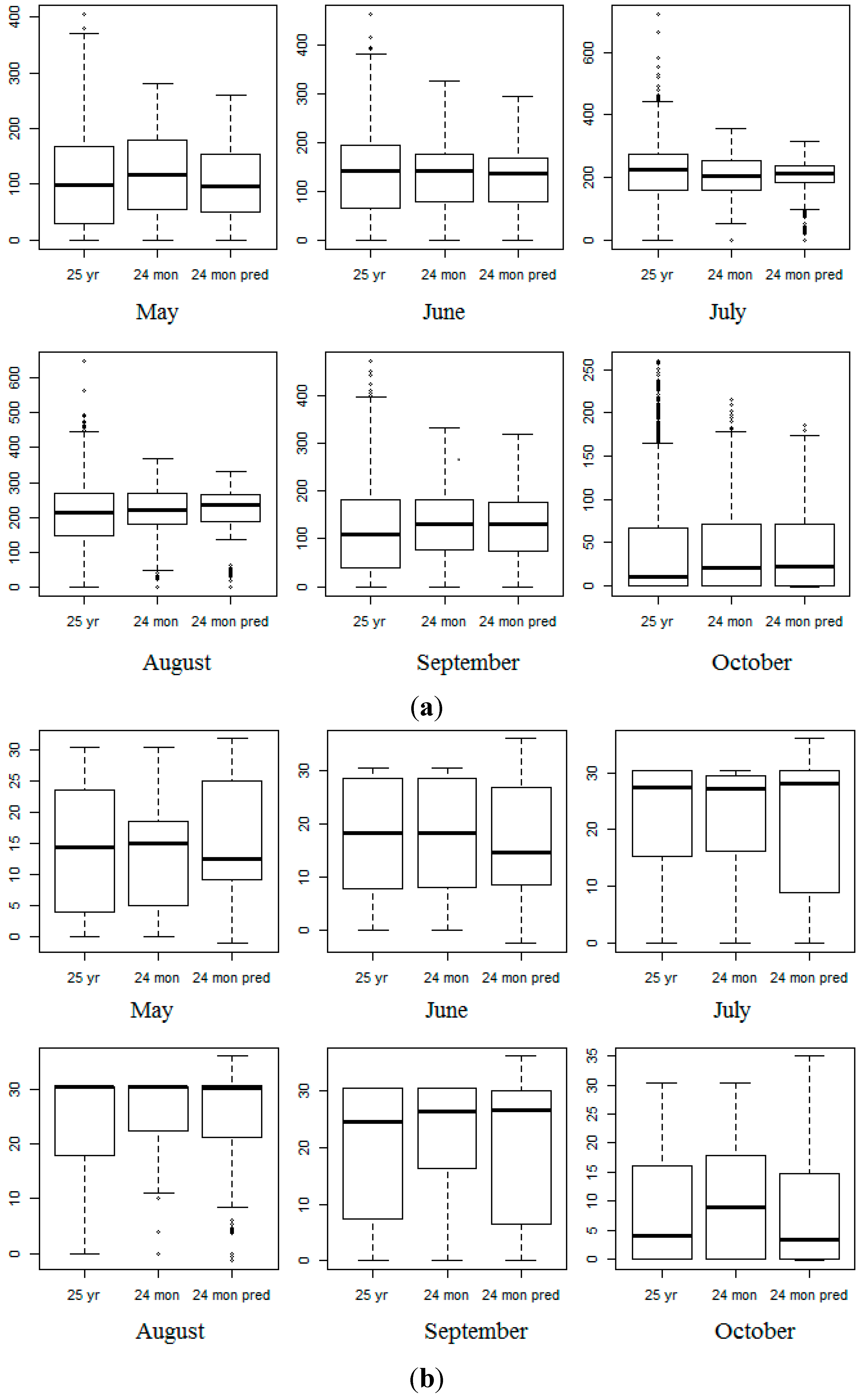
The prediction throughout the study area shows a slight underestimation of the precipitation in the dryer months and overestimation in the much wetter months and variability is always a little underestimated (Figure 4a). The number of rain days is always underestimated and the estimated variability tends to be too large compared to the 24 months of NCEP-CRU data (Figure 4b).

The months of May and June have the highest RMSE (Figure 5a,b). The predicted precipitation for July, August and September has the lowest RMSE suggesting that while these wet months tend to be over predicted, the prediction is actually quite good (Figure 5a) because of the significant agreement between the prediction and the reference data. The general underestimation of the number of rain days is reflected in a relatively high RMSE in particular for the dryer months May, June and October (Figure 5b).

Figure 4. Monthly means and variabilities throughout the study area of the 25 years (1980–2004), 2005 and 2006 NCEP-CRU data and 2005–2006 model predictions of (a) monthly rainfall in mm and (b) the frequency of the number of rain days in a month (in days) from May–October. The first box (25 yr) shows the 25-year data used in making the 24 months prediction into the future, “24 mon” is the 24 months reference data and “24 mon pred” is the prediction. The values are inclusive of all grids for the months plotted.

Figure 4. Monthly means and variabilities throughout the study area of the 25 years (1980–2004), 2005 and 2006 NCEP-CRU data and 2005–2006 model predictions of (a) monthly rainfall in mm and (b) the frequency of the number of rain days in a month (in days) from May–October. The first box (25 yr) shows the 25-year data used in making the 24 months prediction into the future, “24 mon” is the 24 months reference data and “24 mon pred” is the prediction. The values are inclusive of all grids for the months plotted.

Figure 5. RMSE between the 24-month NCEP-CRU and 24-month predictions of (a) monthly rainfall in mm and (b) the frequency of the number of rain days in a month (in days) from May–October. The axes show the latitude and longitude coordinates in degrees.

Figure 5. RMSE between the 24-month NCEP-CRU and 24-month predictions of (a) monthly rainfall in mm and (b) the frequency of the number of rain days in a month (in days) from May–October. The axes show the latitude and longitude coordinates in degrees.

Figure 6. P-values of a Student’s t-test between standard normal deviates of the prediction and standard normal deviates of the means of the long-term monthly data used for the prediction. The months used for this test at each grid scale were August–October.

Figure 6. P-values of a Student’s t-test between standard normal deviates of the prediction and standard normal deviates of the means of the long-term monthly data used for the prediction. The months used for this test at each grid scale were August–October.

Figure 7. The F-skill values of (a) monthly rainfall in mm and (b) the frequency of the number of rain days in a month (in days) from May–October. The axes show the latitude and longitude coordinates in degrees.

Figure 7. The F-skill values of (a) monthly rainfall in mm and (b) the frequency of the number of rain days in a month (in days) from May–October. The axes show the latitude and longitude coordinates in degrees.

The study wanted to know parts of the study area where there are significant differences between the prediction and long-term means of the monthly data used for the prediction and where they are not. A Student’s t-test was used to determine whether the means of the monthly standard normal deviates of the prediction was different from the means of the standard normal deviates of the long term monthly means of the data used for the prediction. The formulated null hypothesis states that there is no significant difference between the means of the standard normal deviates of the prediction and the standard normal deviates of the long term mean. The null hypothesis will be rejected in favor of the alternative hypothesis if p < 0.05. The Student’s t-test was carried out at grid level using the months that fall within the wet season (May–October), however, in the process of carrying out the test the months of August–October gave the best results (Figure 6). Because of the shortness of the prediction it was not possible to make the student’s t-test on a selected month for instance June or July only in each year as there will be only two variables in each case to test. Results of the grid level test for the months of August–October for monthly rainfall amounts show p < 0.05 in many parts of the study area. However, for monthly rainfall frequency fewer grid cells have p < 0.05.

The grid differences between the prediction and the reference data and the performance of the prediction in comparison with the long term mean was carried out using the forecast skill (Figure 7). Areas where the prediction performed better than the long term mean have positive values, areas where the prediction underperformed have negative values and where the prediction replicated the long term mean have values of zero.

4. Discussion

In this study it was shown that spatial and temporal variability of rainfall increases northwards in each of the months in the wet season (May–October) similar to the findings by [7,17]. The CV and regression slopes obtained here show that the decrease in monthly rainfall amounts and frequency in the wet season is mostly in the months following the onset of rainfall (May, June, and July), which is similar to the results of previous studies on rainfall trends and dry spells in the study area. The main difference from previous studies is that in this study the decreasing trend over the 27-year period was mostly confined to the sub-humid part of the study area south of latitude 12° North. The reduction in rain days per month during this period found here is consistent with the findings of [1,4], who showed an increasing length of dry spells in the study area. The decreasing and erratic frequency and amount of rainfall at the onset of the wet season found here could be related to the rapid land use and land cover change experienced in the West African sub-region since the early turn of the 20th century as investigated by [16]. A high inter-annual variation of rainfall in the months after the onset of rainfall has serious implications for rain-fed agriculture in relation to the timing of planting of crops. An increasing likelihood of water shortages both from surface and ground water sources in the study area was reported by [2]. The highest CV found by [2] was in October. Increasing trends in the amount and frequency of rainfall in October were less than the trends for those months at the peak of the wet season (August–September) [2].

The results of Kolmogorov Smirnov test (plots not shown) for the significance in the agreement between the prediction and the reference data increases as the wet season progresses, reaching a peak in the month of September. The significance of the agreement also has a latitudinal gradient generally reducing northward. This exposes the weakness of the model in making prediction in highly varying conditions typical in the region especially at the onset of the wet season. The performance of the prediction was further evaluated in order to determine periods where the prediction fitted the observations better and whether the model is doing much better than simply replicating the long term mean. The Bland-Altman plots suggest much narrower differences between the predictions and the reference data at the peak of the wet season in August. Larger differences between the reference NCEP-CRU data and the ARIMA model’s prediction are in months at the onset of the wet season and in months with high temporal variability (like July). In particular, the comparison of the RMSE of the ARIMA prediction and the climatology, as well as the evaluation of the standard deviates show that the ARIMA model did well in predicting monthly rainfall amounts and to a lesser degree frequency in most of the months in the wet season in the study area in the sense that it provided a better prediction than the long term mean. It is also an indication that the model has memory. However, the model was least successful in predicting the amount of precipitation in the months of May, June, and October at the onset and towards the end the wet season. Those three months have the highest CV. The low performance of the model in making predictions in the dryer months of the wet season and months with higher variability in rainfall amounts and frequency indicates a weakness of the model in making predictions under such conditions.

Similar to other findings in this study, the level of agreement between the NCEP-CRU and predictions generally has a latitudinal gradient and increases southwards.

5. Summary and Conclusions

Because of the frequent droughts in North-eastern Nigeria in the past 60 years this study examined the temporal variability and temporal trends of monthly rainfall amounts and frequency over the 27-year period of 1980–2006. The performance of the ARIMA model in making monthly rainfall prediction was analyzed. The results of the analysis were presented in spatially distributed form.

This study identified those parts of the study area with high rainfall variability, and increasing or decreasing temporal trends. Temporal variability show latitudinal gradient increasing northwards and generally decreasing as the wet season progresses. Temporal trends in monthly rainfall over the 27-year period suggest decreasing trends in the months after the onset of rainfall. There is an increasing trend in rainfall amounts and frequency towards the middle of the wet season especially in northern parts. These results can be used by stakeholders with interests in rain-fed agricultural schemes especially in decision making for the timing of planting of crops, selecting the appropriate variety of crops to plant and in water management schemes.

The strengths and weaknesses of the ARIMA model in predicting monthly rainfall variables were assessed. The findings show significant agreement between the prediction and the reference data increases as the wet season progresses and reaches a peak in the month of September after the peak of the wet season. Despite the insignificant agreement between the prediction and the reference data in many parts of the study area especially in areas with high temporal variability the study was able to establish that the model did much better than simply replicating the long term mean of the NCEP-CRU data used in making the prediction. The model performed less well during the onset of the wet season and in dryer regions in the north a manifestation of the weakness of the model if it is to be used for predicting the onset and cessation of the wet season. Because of the large errors between the prediction and the reference data specifically at parts of the study area of high temporal variability the model cannot be recommended as a viable tool for predicting rainfall in these parts of study area. The model nevertheless provides even in those months a better prediction of rainfall amount than the long term mean (climatology). Overall, the ARIMA model can be used to provide some guidance for planning, depending though on the area and the month. The performance of the model can be further assessed using different rainfall datasets and statistical techniques. Future studies should explore the use of other models in predicting rainfall variables in the study area such as non-linear regression and artificial neural networks. Comparing the performance of a range of models will assist in making better predictions to support decision-making and reducing losses in rain-fed agricultural production in the study area.