Linear and Non-Linear Approaches for Statistical Seasonal Rainfall Forecast in the Sirba Watershed Region (SAHEL)

Abstract
:1. Introduction
2. Review of the Main Drivers of the Sahelian Rainfall Variability
3. Materials and Methods
3.1. Study Area

3.2. Climate and Atmospheric Data

| Station number (code) | Station name | Longitude (degrees: °) | Latitude (degrees: °) | Country |
|---|---|---|---|---|
| 320006 | Torodi | 1.80 | 13.12 | Niger |
| 320002 | Tera | 0.82 | 14.03 | Niger |
| 320004 | Tillaberi | 1.45 | 14.20 | Niger |
| 320005 | Gotheye | 1.58 | 13.82 | Niger |
| 200082 | Boulsa | −0.57 | 12.65 | Burkina Faso |
| 200026 | Dori | 0.03 | 14.03 | Burkina Faso |
| 200085 | Bogande | 0.13 | 12.98 | Burkina Faso |
| 200048 | Dakiri | −0.27 | 13.30 | Burkina Faso |
| 200024 | Gorgadji | −0.52 | 14.03 | Burkina Faso |
| 200086 | Piela | −0.13 | 12.70 | Burkina Faso |
| 200047 | Tougouri | −0.52 | 13.65 | Burkina Faso |
(a) Zonal Wind and Meridional Wind
(b) Air Temperature
(c) SST
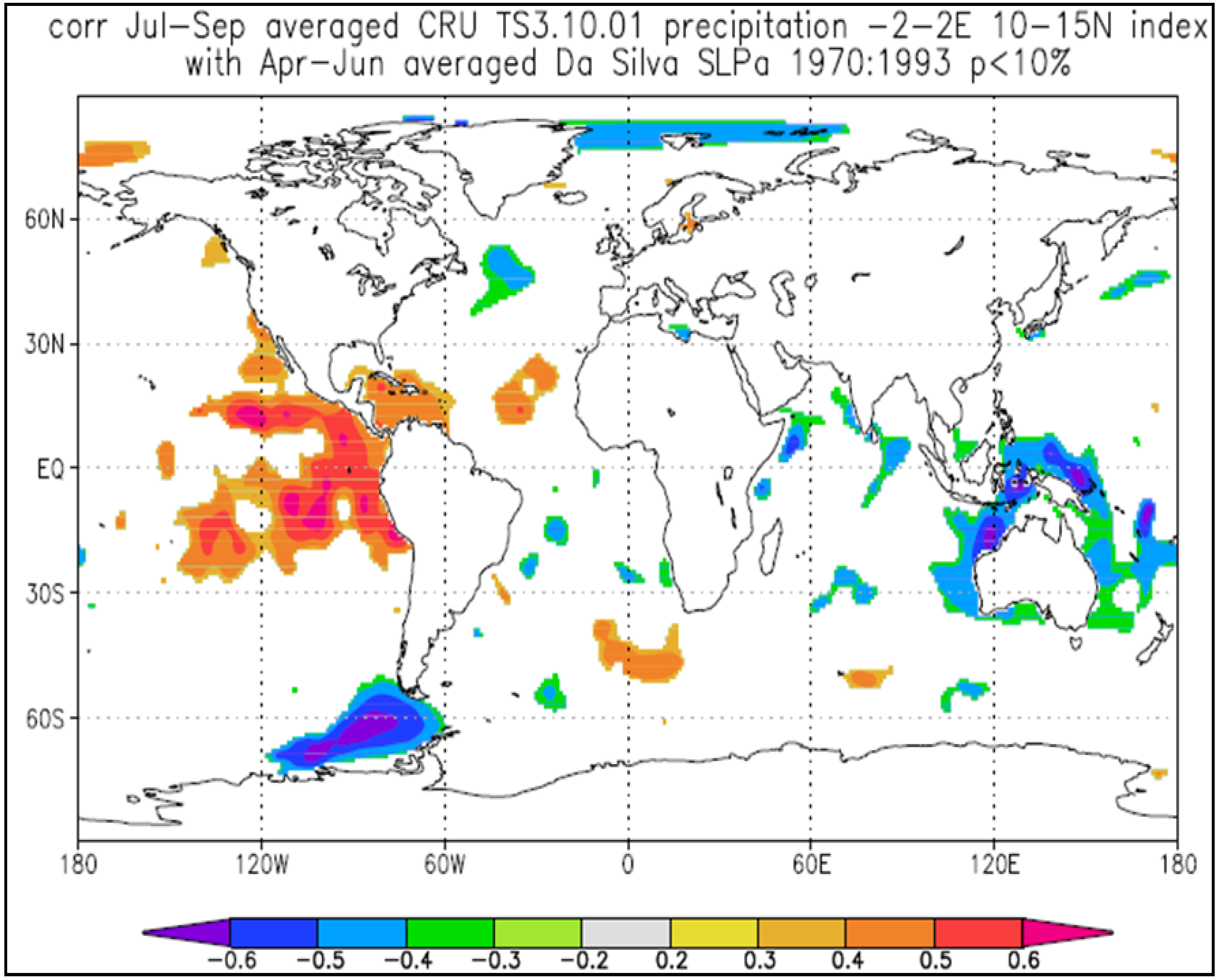
(d) SLP
(e) RHUM
3.3. Selection of Predictors and Optimal Lag Time
| Parameter | Units | Level | Reference Data | Spatial coverage | Regions of the Predicto rs | Temporal Coverage |
|---|---|---|---|---|---|---|
| Sea level pressures (SLP) | Pa/s | 1000 hPa | NCEP 2 | 2.5° × 2.5° grid 15N–45S, 60W–10E | Atlantic ocean | 1979/01/01 to 2013/08/31 |
| Air temperature (AirTemp) | °K | 1000 hPa | NCEP 2 | 2.5° × 2.5° grid 20N–15S, 120E–70W | Pacific ocean | 1979/01/01 to 2013/08/31 |
| Meridional wind (VWND) | m/s | 1000 hPa | NCEP 2 | 2.5° × 2.5° grid 90N–90S, 0–180W | Sahel (Easterly jet) | 1979/01/01 to 2013/08/31 |
| Zonal wind (UWND) | m/s | 1000 hPa | NCEP 2 | 2.5° × 2.5° grid 30N–25S 10W–10E | Sahel (Easterly jet) | 1979/01/01 to 2013/08/31 |
| Relative humidity (RHUM) | % | 1000 hPa | NCEP 2 | 2.5° × 2.5° grid 40N–30N, 20E–35E | Mediterranean basin | 1979/01/01 to 2013/08/31 |
| Sea surface temperature (SST) | °C | Surface | NOAA NCDC ERSST version3b | 2° × 2° grid 39N–15S, 60W–15E | Atlantic ocean | 1854/01/01 to 2013/08/31 |
| Climatic research unit rainfall (CRU) | mm | Surface | CRU | 0.5° × 0.5° grid 2°W–2°E, 10°N–15°N | January 1901 to December 2012 |
- (a)
- For each year Y that the predictor was available,
- (i)
- The predictor of year Y-1 was removed from the predictor grid;
- (ii)
- The rainfall of year Y was removed from the rainfall data set;
- (iii)
- A coefficient of correlation (R) is used to screen the remaining predictor data: a correlation analysis between the predictor at each grid point and the rainfall was computed and its level of significance (P-value <0.05) was assessed. Once the correlation was not significant, the grid point was discarded. The remaining grid points were then ordered decreasingly;
- (iv)
- Afterward, a principal component analysis (PCA) was applied on the retained predictor gridded data from the previous step to reduce the number of predictors;
- (v)
- Since PCA gave rise to more sets of new predictor data, a stepwise regression (5% confidence interval) was used to keep only grid points with high predictive power;
- (vi)
- A linear regression was fitted between the predictors and precipitation time series;
- (vii)
- The fitted linear regression was used to simulate the rainfall of year Y. If predictor and rainfall were in the same year (Year Y), only predictor and rainfall time series for that year were removed in the first step.
- (b)
- Then, the coefficient of determination (R2), Nash-Sutcliffe coefficient (Nash), and Hit-Rate scores (HIT) were computed to estimate the model's performance.

3.4. Linear Approach
3.5. Non-Linear Approach
3.5.1. Non-Linear Principal Component Analysis


3.5.2. Feedforward Neural Network
4. Results and Discussions
4.1. Selected Predictors and Lag Time Period
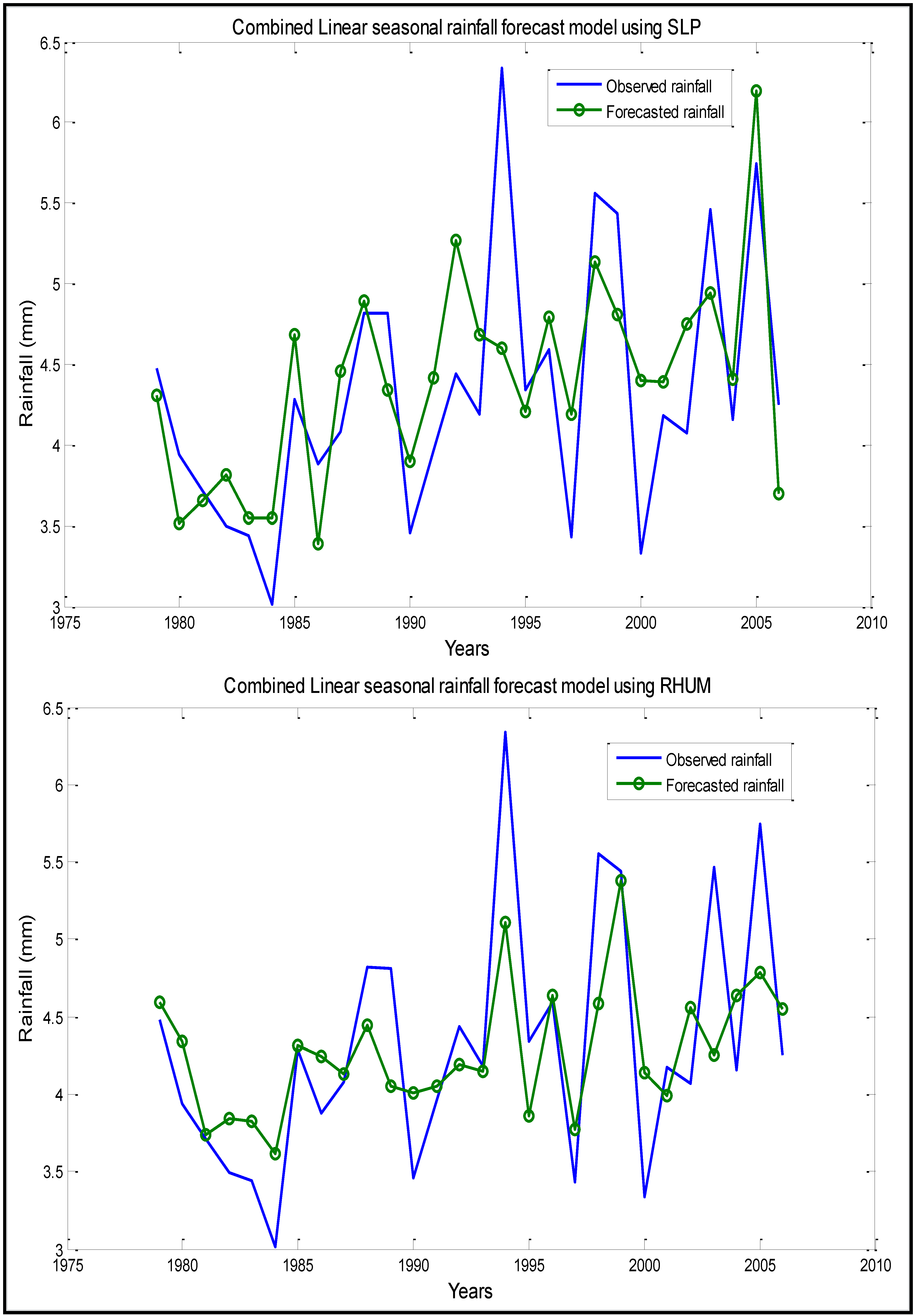
4.2. Seasonal Rainfall Forecast

| PREDICTOR | NMAX* | R2 | Nash coef. | HIT Score | Best period M1-M2** | Lag period |
|---|---|---|---|---|---|---|
| Sea Level Pressure (SLP) at 1000hPa | 50 | 0.48 | 0.46 | 60.71 | 17-18 | 0 |
| Relative Humidity (RHUM) at 1000hPa | 80 | 0.58 | 0.52 | 64.29 | 10-10 | 8 months |
| Air Temperature (AirTemp) at 1000hPa | 10 | 0.530 | 0.527 | 67.86 | 1-4 | 7 months |
| Meridional Wind (VWND) at 1000hPa | 170 | 0.31 | 0.28 | 53.57 | 5-5 | 8 months |
| Zonal Wind(UWND) at 1000hPa | 190 | 0.33 | 0.324 | 71.43 | 11-11 | 7 months |
| Sea surface temperature (SST) | 30 | 0.43 | 0.34 | 58.54 | 3-6 | 12 months |
| PREDICTOR | R2 | NASH | HIT score | Lag time Period |
|---|---|---|---|---|
| Sea Level Pressure (SLP) at 1000hPa | 0.32 | 0.31 | 53.57 | 9 months |
| Relative Humidity (RHUM) at 1000hPa | 0.36 | 0.36 | 53.57 | 7 months |
| Air Temperature (AirTemp) at 1000hPa | 0.46 | 0.45 | 60.71 | 8 months |
| Predictors | R2 | Nash | HIT score (%) | Lag time (months) |
|---|---|---|---|---|
| AirTemp | 0.26 | 0.20 | 48.24 | 4 |
| RHUM | 0.18 | 0.10 | 29.12 | 4 |
| SLP | 0.21 | 0.09 | 18.03 | 2 |
| SST | 0.18 | 0.044 | 11.49 | 5 |


5. Conclusions
Acknowledgements
Author Contributions
Conflicts of Interest
References
- Gado Djibo, A.; Seidou, O.; Karambiri, H.; Sittichock, K.; Paturel, J.E.; Saley, H.M. Development and assessment of non-linear and non-stationary seasonal rainfall forecast models for the Sirba watershed, West Africa. J. Hydrol. Reg. Stud. 2015, 4, 134–152. [Google Scholar] [CrossRef]
- Sarr, M.A.; Gachon, P.; Seidou, O.; Bryant, C.R.; Ndione, J.A.; Comby, J. Inconsistent linear trends in Senegalese rainfall data. Hydrol. Sci. J. 2014. [Google Scholar] [CrossRef]
- Sarr, M.A.; Zoromé, M.; Seidou, O.; Bryant, C.R.; Gachon, P. Recent trends in selected extreme precipitation indices in Senegal-A changepoint approach. J. Hydrol. 2013, 505, 326–334. [Google Scholar] [CrossRef]
- Sittichok, K.; Gado Djibo, A.; Seidou, O.; Saley, H.M.; Karambiri, H.; Paturel, J. Statistical seasonal rainfall and streamflow forecasting for the Sirba watershed, using sea surface temperature. Hydrol. Sci. J. 2014. [Google Scholar] [CrossRef]
- Samimi, C.; Fink, A.H.; Paeth, H. The 2007 flood in the Sahel: causes, characteristics and its presentation in the media and FEWS NET. Nat. Hazards Earth Syst. Sci. 2012, 12, 313–325. [Google Scholar] [CrossRef]
- Brooks, N. Drought in the African Sahel: Long term perspectives and future prospects; University of East Anglia: Norwich, UK, 2004. [Google Scholar]
- Amadou, A.; Gado Djibo, A.; Seidou, O.; Sittichok, K.; Seidou Sanda, I. Changes to flow regime on the Niger River at Koulikoro under a changing climate. J. Hydrol. Sci. 2014. [Google Scholar] [CrossRef]
- Ibrahim, B.; Karambiri, H.; Polcher, J.; Yacouba, H.; Ribsttein, P. Changes in rainfall regime over Burkina Faso under the climate change conditions simulated by 5 regional climate models. Clim. Dyn. 2014, 42, 1363–1381. [Google Scholar] [CrossRef]
- Le Barbe, L.; Lebel, T.; Tapsoba, D. Rainfall variability in West Africa during the years 1950–90. J. Clim. 2002, 15, 187–202. [Google Scholar] [CrossRef]
- Janicot, S.; Trzaska, S.; Poccard, I. Summer Sahel-ENSO teleconnection and decadal time scale SST variations. Clim. Dyn. 2001, 18, 303–320. [Google Scholar] [CrossRef]
- Fontaine, B.; Janicot, S. Sea surface temperature fields associated with West African rainfall anomaly types. J. Clim. 1996, 9, 2935–2940. [Google Scholar] [CrossRef]
- Folland, C.K.; Palmer, T.N.; Parker, D.E. Sahel rainfall and worldwide sea temperature 1901–1985. Nature 1986, 320, 602–607. [Google Scholar] [CrossRef]
- Hastenrath, S. Decadal scale changes of the circulation in the tropical Atlantic sector associated with Sahel drought. Int. J. Climatol. 1990, 20, 459–472. [Google Scholar] [CrossRef]
- Lamb, P.J. West African water variations between recent contrasting Subsaharan droughts. Tellus 1983, 35, 198–212. [Google Scholar] [CrossRef]
- Lamb, P.J.; Peppler, R.A. Further case studies of tropical Atlantic surface atmospheric and oceanic patterns associated with sub-Saharan drought. J. Clim. 1992, 5, 476–488. [Google Scholar] [CrossRef]
- Nicholson, S.E. Rainfall and atmospheric circulation during drought periods and wetter years in West Africa. Mon. Wea. Rev. 1981, 109, 2191–2208. [Google Scholar] [CrossRef]
- Nicholson, S.E. Land surface processes and Sahel climate. Rev. Geophys. 2000, 38, 117–139. [Google Scholar] [CrossRef]
- Nicholson, S.E. The West African Sahel: A review of recent studies on the rainfall regime and its interannual variability. ISRN Meteor. 2013, 2013, 453–521. [Google Scholar] [CrossRef]
- Kwon, H.H.; Brown, C.; Xu, K.; Lall, U. Seasonal and annual maximum streamflow forecasting using climate information: application to the Three Gorges Dam in the Yangtze River basin, China. Hydrol. Sci. J. 2009, 54, 582–595. [Google Scholar] [CrossRef]
- Liu, Z.; Alexander, M. Atmospheric bridge, oceanic tunnel, and global climatic teleconnections. Rev. Geograph. 2007, 45, 1–34. [Google Scholar] [CrossRef]
- Gaetani, M.; Fontaine, B. Interaction between the West African Monsoon and the summer Mediterranean climate: An overview. Fisica de la Tierra 2013, 25, 41–55. [Google Scholar]
- Jung, T.; Ferranti, L.; Tompkins, A.M. Response to the summer 2003 Mediterranean SST anomalies over Europe and Africa. J. Cimate 2006, 19, 5439–5454. [Google Scholar]
- Camberlin, P.; Janicot, S.; Poccard, I. Seasonality and atmospheric dynamics of the teleconnection between African rainfall and tropical sea-surface temperature: Atlantic VS. ENSO. Int. J. Clim. 2001, 21, 973–1005. [Google Scholar] [CrossRef]
- Rowell, D.P. Teleconnections between the tropical Pacific and the Sahel. Q. J. R. Meteorol. Soc. 2001, 127, 1683–1706. [Google Scholar] [CrossRef]
- Chase, T.N.; Pielke, S.R.; Avissar, R. Teleconnections in the Earth System. Encyclopedia of Hydrological Sciences. Available online: http://onlinelibrary.wiley.com/doi/10.1002/0470848944.hsa190/pdf (accessed on 12 August 2014).
- Ndiaye, O.; Ward, M.N.; Thiaw, W.M. Predictability of seasonal Sahel rainfall using GCMs and lead-time improvement through the use of a couple model. J. Clim. 2011, 24, 1931–1949. [Google Scholar] [CrossRef]
- Bouali, L. Prévisibilité et Prévision Statistico-Dynammique des Saisons des Pluies Associées à la Mousson Ouest Africaine à Partir d’Ensembles Multi-modèLes. Ph.D. Thesis, Université de Bourgogne, Bourgogne, France, 2009. [Google Scholar]
- Garbrecht, J.D.; Schneider, J.M.; Van Liew, M.W. Monthly runoff predictions based on rainfall forecasts in a small Oklahoma Watershed. J. Am. Water Resour. Assoc. 2007, 42, 1285–1295. [Google Scholar] [CrossRef]
- Tuteja, N.K.; Shin, D.; Laugesen, R.; Khan, U.; Shao, Q.; Wang, E.; Li, M.; Zheng, H.; Kuczera, G.; Kavetski, D.; et al. Experiment evaluation of the dynamic seasonal streamflow forecasting approach; Bureau of Meteorology: Melbourne, Vic, Australia, 2011.
- Chiew, F.H.S.; McMahon, T.A. Global ENSO-streamflow teleconnection, streamflow forecasting and interannual variability. Hydrol. Sci. J. 2002, 47, 505–522. [Google Scholar] [CrossRef]
- Ndiaye, O.; Goddard, L.; Ward, M.N. Using regional wind fields to improve general circulation model forecasts of July-September Sahel rainfall. Int. J. Clim. 2009, 29, 1262–1275. [Google Scholar] [CrossRef]
- Wang, E.; Zhang, Y.; Luo, J.; Chiew, F.; Wang, Q.J. Monthly and seasonal streamflow forecasts using rainfall-runoff modeling and historical weather data. Water Resour. Res. 2011, 47, 1–13. [Google Scholar] [CrossRef]
- Yossef, N.C.; Winsemius, H.; Weerts, A.; Beek, R.V.; Bierkens, F.P. Skill of global seasonal streamflow forecasting system, relative roles of initial conditions and meteorological forcing. Water Resour. Res. 2013, 49, 4687–4699. [Google Scholar] [CrossRef]
- Mohino, E.; Rodriguez-Fonseca, B.; Mechoso, C.R.; Gervois, S.; Ruti, P.; Chauvin, F. Impacts of the tropical Pacific/Indian Oceans on the seasonal cycle of the West African monsoon. J. Clim. 2011, 24, 3878–3891. [Google Scholar] [CrossRef]
- Rodriguez-Fonseca, B.; Janicot, S.; Mohino, E.; Losada, T.; Bader, J.; Caminade, C.; Chauvin, F.; Fontaine, B.; Garcia-Serrano, J.; Gervois, S.; et al. Interannual and decadal SST-forced responses of the West African monsoon. Atmos. Sci. Lett. 2011, 12, 67–74. [Google Scholar] [CrossRef]
- Singh, O.P. Cause-effect relationships between sea surface temperature, precipitation and sea level along the Bangladesh coast. Theor. Appl. Clim. 2001, 68, 233–243. [Google Scholar] [CrossRef]
- Garcia-Serrano, J.; Doblas-Reyes, F.J.; Haarsma, R.J.; Polo, I. Decadal prediction of the dominant West African monsoon rainfall modes. J. Geophys. Res. Atmos. 2013, 118, 5260–5279. [Google Scholar] [CrossRef]
- Philippon, N.; Doblas-Reyes, F.J.; Ruti, P.M. Skill, reproducibility and potential predictability of the West African monsoon in coupled GCMs. Clim. Dyn. 2010, 35, 53–74. [Google Scholar] [CrossRef]
- Rodrigues, L.R.L.; Garcia-Serrano, J.; Doblas-Reyes, F. Seasonal prediction of the intraseasonal variability of the West African monsoon precipitation. Fisica de la Tierra 2013, 25, 73–87. [Google Scholar]
- Sultan, B.; Janicot, S.; Diedhiou, A. The West African monsoon dynamics. Part I: Documentation of intraseasonal variability. J. Clim. 2003, 16, 3389–3406. [Google Scholar]
- Marteau, R. Cohérence Spatiale et prEvisibilité Potentielle des Descripteurs intrasaisonniers de la Saison des Pluies en Afrique Soudano-Sahélienne : Application à la Culture du mil dans la réGion de Niamey. Ph.D. Thesis, Université de Bourgogne, Bourgogne, France, 2010. [Google Scholar]
- Garric, G.; Douville, H.; Déqué, M. Prospects for improved seasonal predictions of monsoon precipitation over Sahel. Int J. Climatol. 2002, 22, 331–345. [Google Scholar] [CrossRef]
- Tippet, M.K.; Giannini, A. Potentially predictable components of African summer rainfall in an SST-forced GCM simulation. J. Clim. 2006, 19, 3133–3144. [Google Scholar] [CrossRef]
- Batté, L.; Déqué, M. Seasonal predictions of precipitation over Africa using coupled ocean-atmosphere general circulation models: Skill of the ENSEMBLES project multimodel ensemble forecasts. Tellus A 2011, 63, 283–299. [Google Scholar] [CrossRef]
- Olivry, J.C. Evolution réCente des réGimes Hydrologiques en Afrique Intertropicale; Presses Universitaires de Nancy: Nancy, France, 1993. [Google Scholar]
- Rowell, D.P.; Folland, C.K.; Maskell, K.; Ward, M.N. Variability of summer rainfall over Tropical North Africa (1906–1992): Observations and modelling. Q. J. R. Meteorol. Soc. 1995, 121, 669–704. [Google Scholar]
- Solomon, A.; Goddard, L.; Kumar, A.; Carton, J.; Deser, C.; Fukumori, I.; Greene, A.M.; Hegerl, G.; Kirtman, B.; Kushnir, Y.; et al. Distinguishing the roles of natural and anthropogenically forced decadal climate variability. Bull. Am. Meteorol. Soc. 2011, 92, 141–156. [Google Scholar] [CrossRef]
- Gaetani, M.; Mohino, E. Decadal prediction of the Sahelian precipitation in CMIP5 simulations. J. Clim. 2013, 26, 7708–7719. [Google Scholar] [CrossRef]
- Hastenrath, S. Interannual variability and annual cycle: Mechanisms of circulation and climate in the Tropical Atlantic Sector. Mon. Weather. Rev. 1984, 112, 1097–1107. [Google Scholar] [CrossRef]
- Druyan, L.M. The sensitivity of sub-Saharan precipitation to Atlantic SST. Clim. Chang. 1991, 18, 17–36. [Google Scholar] [CrossRef]
- Lamb, P.J.; Peppler, R.A. West Africa. In Teleconnections Linking Worldwide Climate Anomalies; Glantz, M.H., Katz, R.W., Nicholls, N., Eds.; Cambridge University Press: Cambridge, England, 1991; pp. 121–189. [Google Scholar]
- Janicot, S. Spatio-temporal variability of West African rainfall. Part II: associated surface and air mass characteristics. J. Clim. 1992, 5, 499–511. [Google Scholar] [CrossRef]
- Janicot, S.; Moron, V.; Fontaine, B. Sahel droughts and ENSO dynamics. Geophys. Res. Lett. 1996, 23, 515–518. [Google Scholar] [CrossRef]
- Moron, V. Guinean and Sahelian rainfall anomaly indices at annual and monthly scales (1933–1990). Int. J. Clim. 1994, 14, 325–341. [Google Scholar] [CrossRef]
- Janicot, S.; Harzallah, A.; Fontaine, B.; Moron, V. West African monsoon dynamics and Eastern Equatorial Atlantic and Pacific SST anomalies (1970–88). J. Clim. 1998, 11, 1874–1882. [Google Scholar] [CrossRef]
- Rowell, D.P. The impact of Mediterranean SSTs on the Sahelian rainfall season. J. Clim. 2003, 16, 849–862. [Google Scholar] [CrossRef]
- Gaetani, M.; Fontaine, B.; Roucou, P.; Baldi, M. Influence of the Mediterranean Sea on the West African monsoon: intraseasonal variability in numerical simulations. J. Geophys. Res. 2010, 115. [Google Scholar] [CrossRef]
- Polo, I.; Ullmann, A.; Roucou, P.; Fontaine, B. Weather regimes in the Euro-Atlantic and Mediterranean sector and relationship with West African rainfall over the period 1989–2008 from a self-organizing maps approach. J. Clim. 2011, 24, 3423–3432. [Google Scholar] [CrossRef]
- Shaman, J.; Tziperman, E. An atmospheric teleconnection linking ENSO and Southwestern European precipitation. J. Clim. 2011, 24, 124–139. [Google Scholar] [CrossRef]
- Lopez-Parages, J.; Rodriguez-Fonseca, B. Multidecadal modulation of El Niño influence on the Euro-Mediterranean rainfall. Geophys. Res. Lett. 2012, 39. [Google Scholar] [CrossRef]
- Webster, P.J.; Magana, V.O.; Palmer, T.N.; Shukla, J.; Tomas, R.A.; Yanai, M.; Yasunari, T. The monsoon: Processes, predictability and prediction. J. Geophys. Res. 1998, 103, 14451–14510. [Google Scholar] [CrossRef]
- Eltahir, E.A.B. Role of vegetation in sustaining large-scale atmospheric circulations in the tropics. J. Geophys. Res. 1996, 101, 4255–4268. [Google Scholar] [CrossRef]
- Philippon, N.; Fontaine, B. The relationship between the Sahelian and previous 2nd Guinean rainy seasons: A monsoon regulation by soil wetness. Ann. Geophys. 2002, 20, 575–582. [Google Scholar] [CrossRef]
- Hall, N.M.J.; Peyrillé, P. Dynamics of the West African Monsoon. J. Phys. IV France 2006, 139, 81–99. [Google Scholar] [CrossRef]
- Zheng, X.; Eltahir, E.A.B. The role of vegetation in the dynamics of West African monsoons. J. Clim. 1998, 11, 2078–2096. [Google Scholar] [CrossRef]
- Wang, G.; Eltahir, E.A.B. Role of vegetation dynamics in enhancing the low frequency variability of the Sahel rainfall. Water Resour. 2000, 36, 1013–1021. [Google Scholar] [CrossRef]
- Zeng, N.; Neelin, J.D.; Lau, K.M.; Tucker, C.J. Enhancement of interdecadal climate variability in the Sahel by vegetation interaction. Science 1999, 286, 1537–1540. [Google Scholar] [CrossRef] [PubMed]
- Cook, K.H. Generation of the African easterly jet and its role in determining West African precipitation. J. Clim. 1999, 12, 1165–1184. [Google Scholar] [CrossRef]
- Douville, H.; Chauvin, F.; Broqua, H. Influence of soil moisture on the Asian and African monsoons. Part I: Mean monsoon and daily precipitation. J. Clim. 2001, 14, 2381–2403. [Google Scholar] [CrossRef]
- Douville, H. Influence of soil moisture on the Asian and African monsoons. Part II: Interannual variability. J. Clim. 2002, 15, 701–720. [Google Scholar] [CrossRef]
- Douville, H. Assessing the influence of soil moisture on seasonal climate variability with AGCMs. J. hydrometeorol. 2003, 4, 1044–1066. [Google Scholar] [CrossRef]
- Mara, F. Développement et analyse des critères de vulnérabilité des populations sahéliennes face à la variabilité du climat: le cas de la ressource en eau dans la vallée de la Sirba au Burkina Faso. Ph.D. Thesis, Université du Québec à Montréal, Montréal, QC, Canada, 2010. [Google Scholar]
- Taweye, A. Contribution à l’étude hydrologique du bassin versant de la Sirba à Garbé-Kourou. Centre Régional AGRHYMET: Ouagadougou, Burkina Faso, 1995. [Google Scholar]
- Ball, J.E.; Luk, K.C. Modeling spatial variability of rainfall over a catchment. J. Hydrol. Eng. 1998, 3, 122–130. [Google Scholar] [CrossRef]
- British Atmospheric Data Centre (BADC). High-Resolution Gridded Datasets (and Derived Products). Available online: http://www.cru.uea.ac.uk/cru/data/hrg/ (accessed on 9 September 2015).
- International Research Institute for Climate and Society (IRI) Data Library. Available online: http://iridl.ldeo.columbia.edu (accessed on 9 September 2015).
- Gallée, H.; Moufouma-Okia, W.; Bechtold, P.; Brasseur, O.; Dupays, I.; Marbaix, P.; Messager, C.; Ramel, R.; Lebel, T. A high-resolution simulation of a West African rainy season using a regional climate model. J. Geophys. Res. 2004, 109. [Google Scholar] [CrossRef]
- Thorncroft, C.; Blackburn, M. Maintenance of the African easterly jet. Q. J. R. Meteorol. Soc. 1999, 125, 763–786. [Google Scholar] [CrossRef]
- Grist, J.P.; Nicholson, S. A Study of the Dynamic Factors Influencing the Rainfall Variability in the West African Sahel. J. Clim. 2001, 14, 1337–1359. [Google Scholar] [CrossRef]
- Janicot, S.; Mounier, F.; Hall, N.M.J.; Leroux, S.; Sultan, B.; Kiladis, G.N. Dynamics of the West African monsoon. Part IV: Analysis of 25-90-Day variability of convection and the role of the Indian monsoon. J. Clim. 2009, 22, 1541–1565. [Google Scholar] [CrossRef]
- Sultan, B. Etude de la Mise en Place de la Mousson en Afrique de l’Ouest et de la Variabilité Intra Saisonnière de la Convection. Applications à la Sensibilité des Rendements Agricoles. Ph.D. Thesis, Université Denis Diderot, Paris, France, 2002. [Google Scholar]
- Nicholson, S.; Grist, J. The seasonal evolution of the atmospheric circulation over West Africa and equatorial Africa. J. Clim. 2003, 16, 1013–1030. [Google Scholar] [CrossRef]
- Fontaine, B.; Louvet, S.; Roucou, P. Definition and predictability of an OLR based West African monsoon onset. Int. J. Climatol. 2008, 28, 1787–1798. [Google Scholar] [CrossRef]
- Flaounas, E.; Janicot, S.; Bastin, S.; Roca, R.; Mohino, E. The role of the Indian monsoon onset in the West African monsoon onset: observations and AGCM nudged simulations. Clim. Dyn. 2012, 38, 965–983. [Google Scholar] [CrossRef]
- Guiavarch, C.; Tréguier, A.M.; Vangriesheim, A. Deep currents in the Gulf of Guinea: Along slope propagation of intraseasonal waves. Ocean Sci. 2009, 5, 141–153. [Google Scholar] [CrossRef]
- Coëtlogon, G.; Janicot, S.; Lazar, A. Intraseasonal variability of the ocean—Atmosphere coupling in the Gulf of Guinea during boreal spring and summer. Q. J. R. Meteorol. Soc. 2010, 136, 426–441. [Google Scholar] [CrossRef]
- Peyrillé, P.; Lafore, J.P. An idealized Two-Dimensional framework to study the West African monsoon. Part II: Large-scale advection and the diurnal cycle. J. Atmos. Sci. 2007, 64, 2783–2803. [Google Scholar] [CrossRef]
- Fontaine, B.; Garcia-Serrano, J.; Roucou, P.; Rodriguez-Fonseca, B.; Losada, T.; Chauvin, F.; Gervois, S.; Sijikumar, S.; Ruti, P.; Janicot, S. Impacts of warm and cold situations in the Mediterranean basins on the West African monsoon: observed connection patterns (1979–2006) and climate simulations. Clim. Dyn. 2010, 35, 95–114. [Google Scholar] [CrossRef]
- Gu, G.; Adler, R. Seasonal evolution and variability associated with the West African monsoon system. J. Clim. 2004, 17, 3364–3377. [Google Scholar] [CrossRef]
- Giannini, A.; Saravanan, R.; Chang, P. Oceanic forcing of Sahel rainfall on interannual to interdecadal time scales. Science 2003, 302, 1027–1030. [Google Scholar] [CrossRef] [PubMed]
- Baldi, M.; Dalu, G.; Maracchi, G.; Pasqui, M.; Cesarone, F. Heat waves in the Mediterranean: A local feature or a larger-scale effect? Int. J. Climatol. 2006, 26, 1477–1487. [Google Scholar] [CrossRef]
- Kalnay, E.; Kanamitsu, M.; Kistler, R.; Collins, W.; Deaven, D.; Gandin, L.; Iredell, M.; Saha, S.; White, G.; Woollen, J.; et al. The NCEP/NCAR 40-year reanalysis project. Bull. Am. Met. Soc. 1996, 77, 437–471. [Google Scholar] [CrossRef]
- Kistler, R.; Kalnay, E.; Collins, W.; Saha, S.; White, G.; Woollen, J.; Chelliah, M.; Ebisuzaki, W.; Kanamitsu, M.; Kousky, V.; et al. The NCEP-NCAR 50-year reanalysis: Monthly means CD-ROM and documentation. Bull. Am. Met. Soc. 2001, 82, 247–268. [Google Scholar] [CrossRef]
- Maheras, P.; Kutiel, H. Spatial and temporal variations in the temperature regime in the Mediterranean and their relationship with circulation during the last century. Int. J. Climatol. 1999, 19, 745–764. [Google Scholar] [CrossRef]
- Lafore, J.; Flamant, C.; Giraud, V.; Guichard, F.; Knippertz, P.; Mahfouf, J.; Mascart, P.; Williams, E. Introduction to the AMMA special issue on “Advances in understanding atmospheric processes over West Africa through the AMMA field campaign”. Q. J. R. Meteorol. Soc. 2010, 136, 2–7. [Google Scholar] [CrossRef]
- Broman, D.; Rajagopalan, B.; Hopson, T. Spatiotemporal variability and predictability of Relative Humidity over West African Monsoon Region. J. Clim. 2014, 27, 5346–5363. [Google Scholar] [CrossRef]
- Scholz, M.; Martin, F.; Joachim, S. Nonlinear principal component analysis: neural network models and applications. In Principal manifolds for Data visualization and dimension reduction; Gorban, A.N., Kegl, B., Wunsch, D.C., Zinovyev, A., Eds.; Springer: Berlin, Germany, 2007; pp. 44–67. [Google Scholar]
- Wu, A.; Hsieh, W.W. The nonlinear Northern Hemisphere atmospheric response to ENSO. Geophys. Res. Lett. 2004, 31. [Google Scholar] [CrossRef]
- Hsieh, W.W. Nonlinear multivariate and time series analysis by neural network methods. Rev. Geophys. 2004, 42. [Google Scholar] [CrossRef]
- Monahan, A.H.; Fyfe, J.C.; Pandolfo, L. The vertical structure of winter time climate regimes of the northern hemisphere extratropical atmosphere. J. Clim. 2003, 16, 2005–2021. [Google Scholar] [CrossRef]
- Diamantaras, K.; Kung, S. Principal Component Neural Networks; Wiley: Hoboken, NJ, USA, 1996. [Google Scholar]
- Jolliffe, I.T.; Stephenson, D.B. Forecast Verification: A Practitioner’s Guide in Atmospheric Science, 2nd ed.; John Wiley & Sons: Hoboken, NJ, USA, 2012. [Google Scholar]
- Tangang, F.T.; Hsieh, W.W.; Tang, B. Forecasting regional sea surface temperatures in the tropical Pacific by neural network models, with wind stress and sea level pressure as predictors. J. Geogr. Res. 1998, 103, 7511–7522. [Google Scholar] [CrossRef]
- Canon, A.J.; Mckendry, I. Forecasting all-India summer monsoon rainfall using regional circulation principal components: A comparison between neural network and multiple regression models. Int. J. Clim. 1999, 19, 1561–1578. [Google Scholar] [CrossRef]
- Badr, H.S.; Zaitchik, B.F.; Guikema, S.D. Application of statistical models to the prediction of seasonal rainfall anomalies over the Sahel. J. Appl. Meteor. Climatol. 2014, 53, 614–636. [Google Scholar] [CrossRef]
- El-Shafie, A.H.; El-Shafie, A.; El-Magzoghi, H.G.; Shehata, A.; Taha, M.R. Artificial neural network technique for rainfall forecasting applied to Alexandria, Egypt. Int. J. Phys. Sci. 2011, 6, 1306–1316. [Google Scholar]
- Ansari, H. Forecasting Seasonal and Annual Rainfall Based on Nonlinear Modeling with Gamma Test in North of Iran. Int. J. Eng. Pract. Res. 2013, 2, 16–29. [Google Scholar]
- Hung, N.Q.; Babel, M.S.; Weesakul, S.; Tripathi, N.K. An artificial neural network for rainfall forecasting in Bangkok, Thailand. Hydrol. Earth Sys. Sci. Discuss. 2008, 5, 183–218. [Google Scholar] [CrossRef]
- Philippon, N. Une Nouvelle Approche Pour la Prévision Statistique des Précipitations Saisonnières en Afrique de l'Ouest et de l'Est: Méthodes, Diagnostics (1968–1998) et Applications (2000–2001). Ph.D. Thesis, Université de Bourgogne, Dijon, France, 2002. [Google Scholar]
© 2015 by the authors; licensee MDPI, Basel, Switzerland. This article is an open access article distributed under the terms and conditions of the Creative Commons Attribution license (http://creativecommons.org/licenses/by/4.0/).
Share and Cite
Djibo, A.G.; Karambiri, H.; Seidou, O.; Sittichok, K.; Philippon, N.; Paturel, J.E.; Saley, H.M. Linear and Non-Linear Approaches for Statistical Seasonal Rainfall Forecast in the Sirba Watershed Region (SAHEL). Climate 2015, 3, 727-752. https://doi.org/10.3390/cli3030727
Djibo AG, Karambiri H, Seidou O, Sittichok K, Philippon N, Paturel JE, Saley HM. Linear and Non-Linear Approaches for Statistical Seasonal Rainfall Forecast in the Sirba Watershed Region (SAHEL). Climate. 2015; 3(3):727-752. https://doi.org/10.3390/cli3030727
Chicago/Turabian StyleDjibo, Abdouramane Gado, Harouna Karambiri, Ousmane Seidou, Ketvara Sittichok, Nathalie Philippon, Jean Emmanuel Paturel, and Hadiza Moussa Saley. 2015. "Linear and Non-Linear Approaches for Statistical Seasonal Rainfall Forecast in the Sirba Watershed Region (SAHEL)" Climate 3, no. 3: 727-752. https://doi.org/10.3390/cli3030727
APA StyleDjibo, A. G., Karambiri, H., Seidou, O., Sittichok, K., Philippon, N., Paturel, J. E., & Saley, H. M. (2015). Linear and Non-Linear Approaches for Statistical Seasonal Rainfall Forecast in the Sirba Watershed Region (SAHEL). Climate, 3(3), 727-752. https://doi.org/10.3390/cli3030727