1. Introduction
The polar regions, especially the Arctic, are critically important to the global climate and they play a vital role in ecosystems as well as the global economy. Because of its importance, government agencies from the eight Arctic countries have been developing national/international strategies to better understand and protect this area. For instance, the US government has stressed the significance of the Arctic region using the slogan “Charting and mapping the Arctic region”. The US National Science Foundation has established a Polar Cyberinfrastructure program to take advantage of the advanced cyberinfrastructure technology to support the analysis of the Arctic/Antarctic climate phenomena and their change [
1,
2,
3,
4]. In recent years, a consensus has been reached by climate scientists that the Arctic climate has exhibited significant changes [
5,
6]. To pinpoint and trace these variances and changes, research has been focusing on analyzing and evaluating observation data on synoptic activity and atmospheric events occurring in this region with statistical methods [
7,
8,
9,
10].
The visualization of spatiotemporal wind data is regarded as the most intuitive and fundamental process in cyclone analysis. It not only draws a graphical illustration of discrete wind data to facilitate the understanding of the cyclone but it also contributes to the viewing of cyclone characteristics. Motivated to provide a robust, multi-dimensional visualization and analysis toolkit for polar scientists exploring and researching the complicated Arctic region, a user-friendly and interactive knowledge-driven visualization system on a web environment is ultimately constructed in our work. The cyclone identification submodule enables scientists to obtain knowledge from raw atmospheric data. The wind simulation submodule, on the other hand, significantly contributes to the validation of knowledge and to eventually solving the challenges of decision-making in North Polar matters.
In the field of scientific data visualization, studies indicate that research topics shift from visualizing small, isolated spatial entities to massive-scale, dynamic data, varying both in spatial and time dimension [
11]. To address this development, many researchers have proclaimed the work with multivariate data sets to be an important task for future visualization research that will require significant advances in developing visualization algorithms. Raphael Fuchs et al. gave us an overview of typical techniques from various disciplines dealing with the complex multi-dimensional scalar, vector, and tensor data sets [
12]. Hesselink et al. indicated four goals for future visualization research [
13]: feature-based representation of data, compromising reduced visual complexity, increased information content and a visualization that matches the concepts of the application area. These goals are still available today. As pointed out by Google’s Eric Schmidt, we are creating as much information every two days as we did from the dawn of civilization up until 2003 [
14]. The situation we face shifts from the lack of data to the “big data” world. How to extract and visualize knowledge from massive spatiotemporal data effectively poses a great challenge [
15].
Furthermore, the analysis and extraction of the raw data are more beneficial to researchers than the capture and visualization of raw data itself. Exemplified in a scenario, climate scientists may have a hypothesis about the atmospheric events from the visualization of climate data and would like to test and verify these assumptions. Knowledge-driven visualization systems meet that requirement and help the scientist to view information, discover knowledge, make a decision and plan for the future. In other words, these systems enable researchers to focus on regions of interest and to detect activity from massive spatiotemporal data over thousands of time steps. In this paper, we leave out a vast amount of work on knowledge extraction by identifying a cyclone from the spatiotemporal climate data, tracking the cyclone and verifying the cyclone trajectory with the dynamic simulation of cyclone characteristics.
The remainder of this paper is organized as follows. In
Section 2, we summarize the previous work on the most important process of the knowledge-driven system—the cyclone identification algorithm and cyclone simulation approach. We then discuss the methodology of cyclone identification in
Section 3. In
Section 4, we briefly discuss the realization of wind simulation with graphics cards and the integration of identification results with a cyclone simulation for result validation.
Section 5 is dedicated to introducing the data we use and analyzing the experimental results, including performance and accuracy. In the last chapter, we conclude the paper with a discussion of our method and the future research of the knowledge-driven visualization system.
2. Related Works
Web-based 3D (three-dimensional) geo-applications have been studied in various research projects using different technology, such as VRML (Virtual Reality Modeling Language), X3D (Extensible 3D) [
16] and WebGL [
17]. However, the 4D (four-dimensional) representation of time-varying phenomena in geo-visualization tools has not yet been thoroughly studied [
18]. Resch identified a number of open research questions including mapping graphic variables to thematic expressivity, representation of the time dimension in 4D geo-applications and implementing a prototypical system to visualize marine spatial data [
18]. Kang reported an empirical study that tested the usefulness of Web-based 4D construction visualization in collaborative construction planning and scheduling [
19]. However, those research projects focus on the 4D representation of the atmospheric phenomenon rather than knowledge extraction from the raw data sets.
Usually, atmospheric phenomenon identification and tracking are more valuable to climate scientists than data visualization. In the field of atmospheric activity identification, Ozer et al. introduced a prototype of activity detection in scientific visualization [
20]. Their goal was to develop a framework and facilitate scientists to model and identify a spatiotemporal pattern from massive data sets. However, current estimates of cyclone variability and cyclone identification methods are usually derived from analyses of surface level pressure (SLP) fields (e.g., the NCEP/NCAR Reanalysis Project) [
21]. These works assimilate observational data into a physical model to produce atmospheric fields. The accuracy of these analyses is severely limited over the oceans. In other research, remote measurements that cover the globe to detect cyclones are used to solve this issue. Scientists attempted to find out suitable features for cyclone identification by gathering statistics from remote sensing data. These data include aerial reconnaissance aircraft data, local radar data and the global scale quickSCAT satellite data. Ho et al. (2008) used the SVM (Support Vector Machine) classifier to identify the cyclone by considering the factor of wind speed, the wind direction, and the direction-to-speed ratio [
22]. It is a feasible approach; however, the robustness of the classifiers should be refined. Much more research is focused on tropical cyclone identification where the characteristics of cyclones are more apparent and noticeable. Nguyen et al. (2014) gave a detailed introduction and evaluation of the tropical cyclone identification methods based on numerical models [
23]. However, polar cyclones we are interested in are smaller and harder to recognize than tropical cyclones. This means some methods for tropical identification may not work in polar cyclone identification.
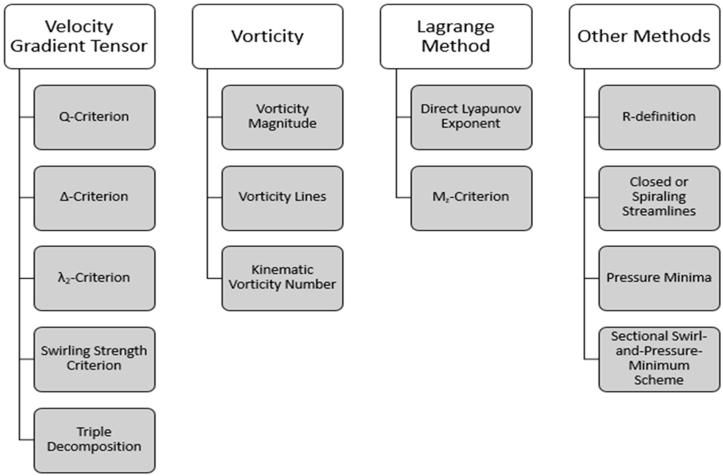
In the field of computational fluid dynamics (CFD), research focuses on identifying fluid vortices. Many classical algorithms have been proposed to identify vortices. The intuitive definitions depict a vortex in terms of closed or spiral streamlines, local pressure minima, and maximum vorticity contours. Holmen (2012) classified these vortex identification methods into four groups [
24].
Figure 1 demonstrates the detailed classification of the four groups. Some representative algorithms are listed in the group.
Vorticity is deemed as one of the most natural choices for cyclone identification criteria since it indicates the physical characteristics of a vortex. However, it has been stressed that the vorticity criterion is limited to cyclone identification due to its failure to distinguish between pure shearing motion and the actual swirling motion. Important criteria have been proposed by analyzing the velocity gradient tensor. Vortex identification algorithms based on the velocity gradient tensor gradually turned into the most widely used local method. However, it is difficult to differentiate cyclones with small vorticity in small shearing flow against cyclones with large vorticity in large shearing flow using the point-wise algorithm based on the velocity gradient tensor. The integration of particle trajectory is necessary within the Lagrange method which makes it computationally expensive. Meanwhile, other methods such as closed or spiral streamline and pressure minima are limited to the specific situation.
In our work, a combination method exploiting the pressure level and velocity is proposed for cyclone identification in order to reduce the limitation of the existing methods. Firstly, the pressure minima criterion is used to filter out noises and generate a potential cyclone eye set. An extra check with velocity direction and triple decomposition follow to identify the actual cyclone eye.
3. Methodology
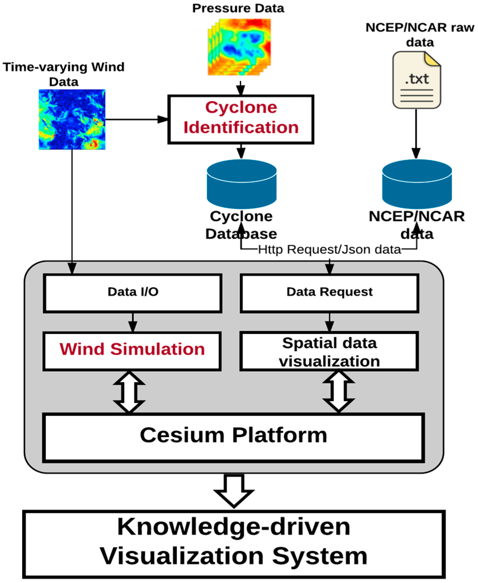
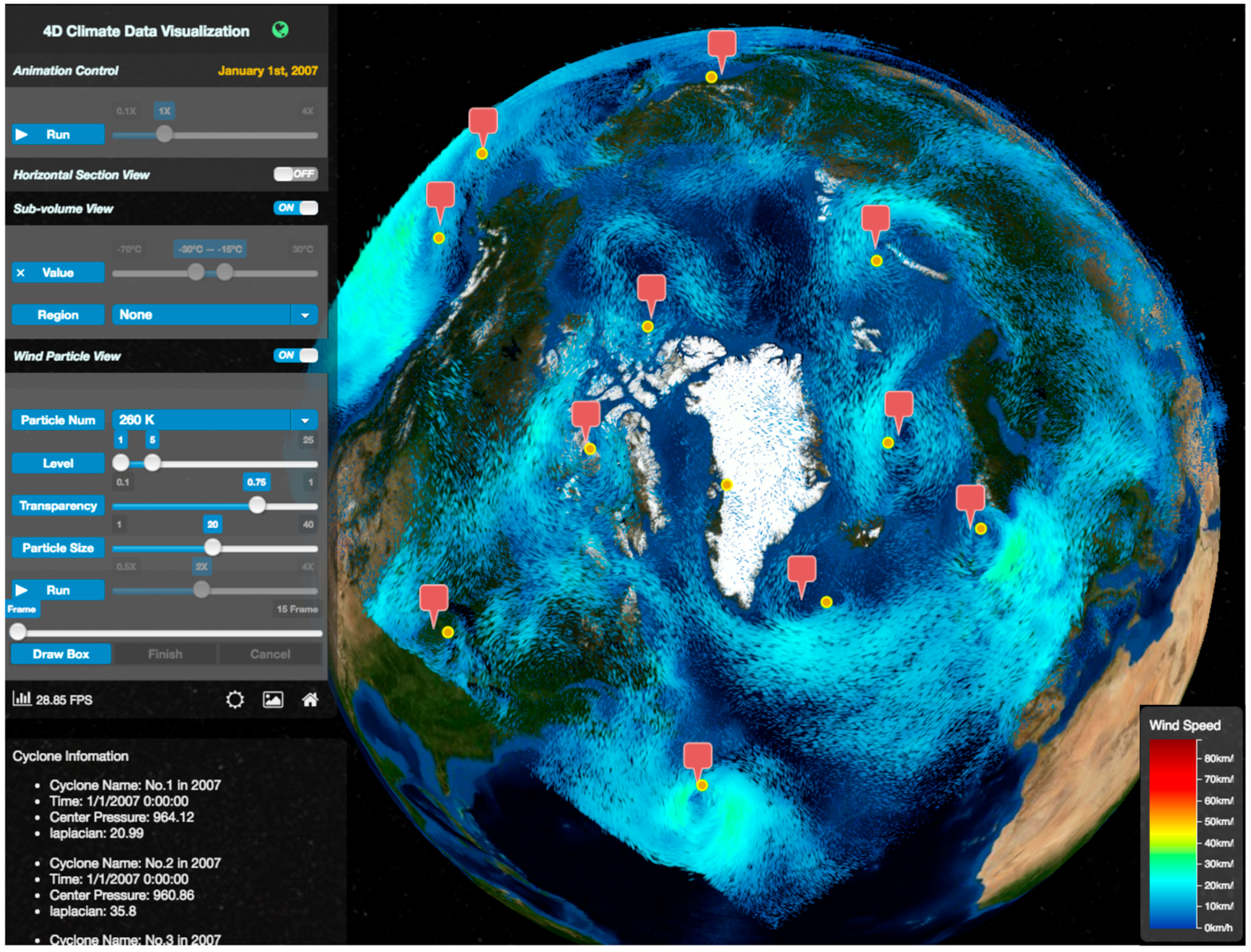
In our work, a user-friendly knowledge-driven visualization system is our goal to facilitate climate analysis. The architecture of the system is demonstrated in
Figure 2. The cyclone identification submodule, which is the most significant submodule in the system, enables users to filter and extract an atmospheric phenomenon from massive climate data. Rather than by drawing a geometric point on a digital earth as a representation for a cyclone, the wind simulation submodule provides a more vivid approach to validate the identification output.
Generally, in knowledge-driven visualization systems, scientists may prefer to discover the atmospheric activity at the North Pole instead of viewing the geometric information. More interest is targeted at the questions “When and where does the activity happen?” and “How long does that activity last?” Polar cyclones, which are a kind of that atmospheric activity, are climatological features that hover near the poles year-round [
25]. The formation of polar cyclones is primarily influenced by the movement of wind and the transfer of heat in the polar region. Hence, more attention will be paid to the methodology of the identification of cyclones from massive time-varying wind field data and tracing the cyclone path. We subsequently leave out a few descriptions on the integration of the extracted cyclone with the wind visualization system.
A polar cyclone is always identified within a low-pressure zone embedded in a large mass of very cold air that lies atop the poles. Since a polar cyclone exists from the stratosphere downward into the mid-troposphere, a variety of pressure levels can be used for polar cyclone identification [
26,
27]. However, each cyclone eye has an extremely minimum pressure in its neighborhood, not vice versa. Hence, augmented techniques are necessary for filtering the potential cyclone eye. Given that we have the pressure data and wind velocity field, a combination of minimum pressure extraction and wind direction filter is used for cyclone identification in our method.
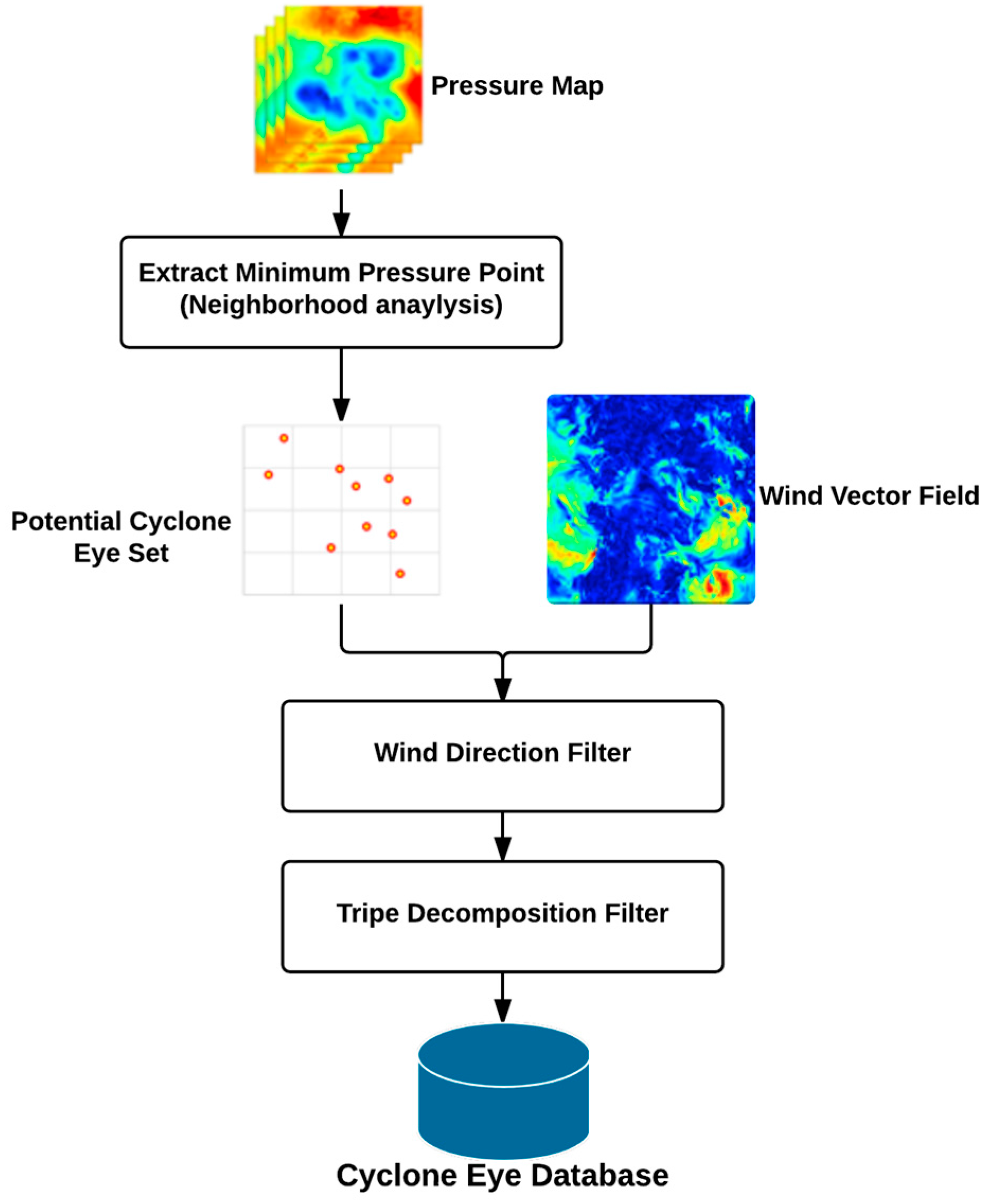
Figure 3 illustrates the flow of our cyclone identification algorithm. First, we extract the minimum pressure in the neighborhood to find the potential cyclone eye. Second, wind field is used to filter out the actual cyclone eye. In our work, a combination of wind direction detection and triple decomposition are exploited to accomplish this goal.
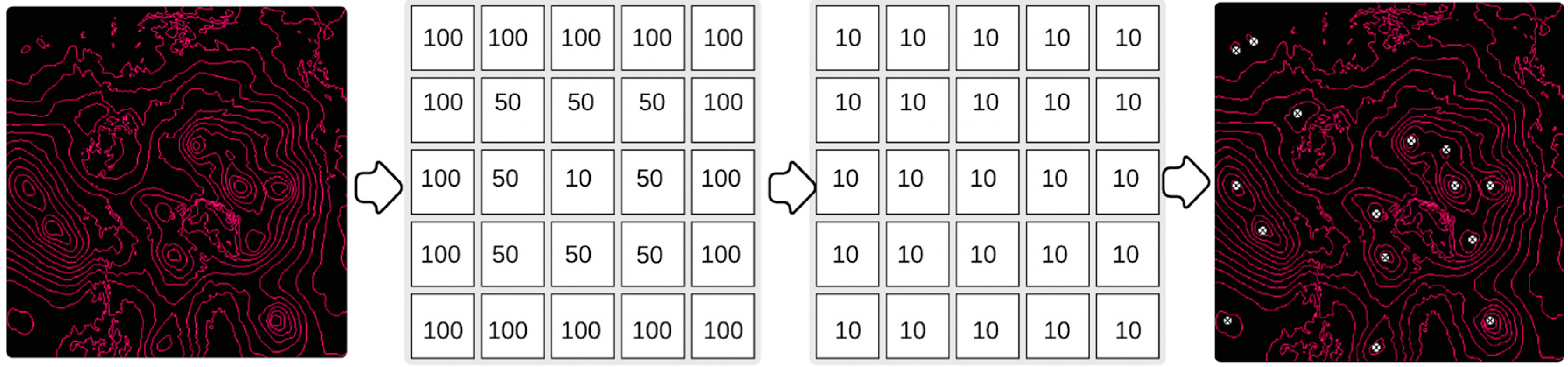
The depression in the pressure map characterized by the minimal pressure value could be identified effectively by performing a neighborhood operation in the spatial analysis [
28]. The threshold range of neighborhood
r should be specified to generate the neighborhood area. Each pixel’s value in the pressure grid is updated with the minimum value in its neighborhood; then a new pressure map is generated. The potential cyclone eye is identified where the pressure value in the original map and the new map are equal.
Figure 4 gives an illustration of this process with
r specified as 5. In our experiments, the neighborhood operation is conducted using GRASS GIS (Geographic Resources Analysis Support System, geographic information system), a free and open-source GIS software suite in Python and the neighborhood range
r = 13. Even though
r is an empirical value, it has a small influence on the outcome due to the spatial distance of two cyclones. After the minimal pressure value filter, a potential cyclone eye set is generated for further filtering purposes.
It appears that the wind direction in the neighborhood of a cyclone eye composes a rotation circle from the physical characteristics. So the noise in the potential cyclone eye set might be filtered out by checking the change pattern of the wind direction within the local neighborhood of a cyclone eye. Four potential scenarios might be found near the potential cyclone eye in the northern hemisphere (seen in
Figure 5). Scenario (a) has the most possibility to be found near the cyclone eye. To filter through these scenarios, a signum operation is carried out on the matrices containing the velocity components in relevant directions. For a potential cyclone eye, its four neighbors—up, down, left and right—are selected for direction filtering.
In each scenario, Y components of velocity are considered with the left and right neighbor; X components with the up and down neighbor. Seen in Equation (1),
U and
V indicate the X component of the velocity and the Y component of the velocity, respectively. If the sum of the signum value of the velocity matrix in the relevant direction equals 0, the direction might compose a rotation. With this principle, we can filter out the wind scenario in
Figure 5d where the wind direction goes in the same direction.
An extra check is conducted to make sure the direction entails a rotation, as there are still three scenarios where the sum of the signum value equals 0. These scenarios are depicted in
Figure 5a–c. To filter out the scenario in
Figure 5b, another check illustrated in Equation (2) is done by checking the sum of the signum values for the left and upper neighbors. However, the scenario in
Figure 5c cannot be filtered out by Equations (1) and (2). This indicates that the velocity data alone cannot distinguish pure shearing motions from the actual swirling motion of a cyclone.
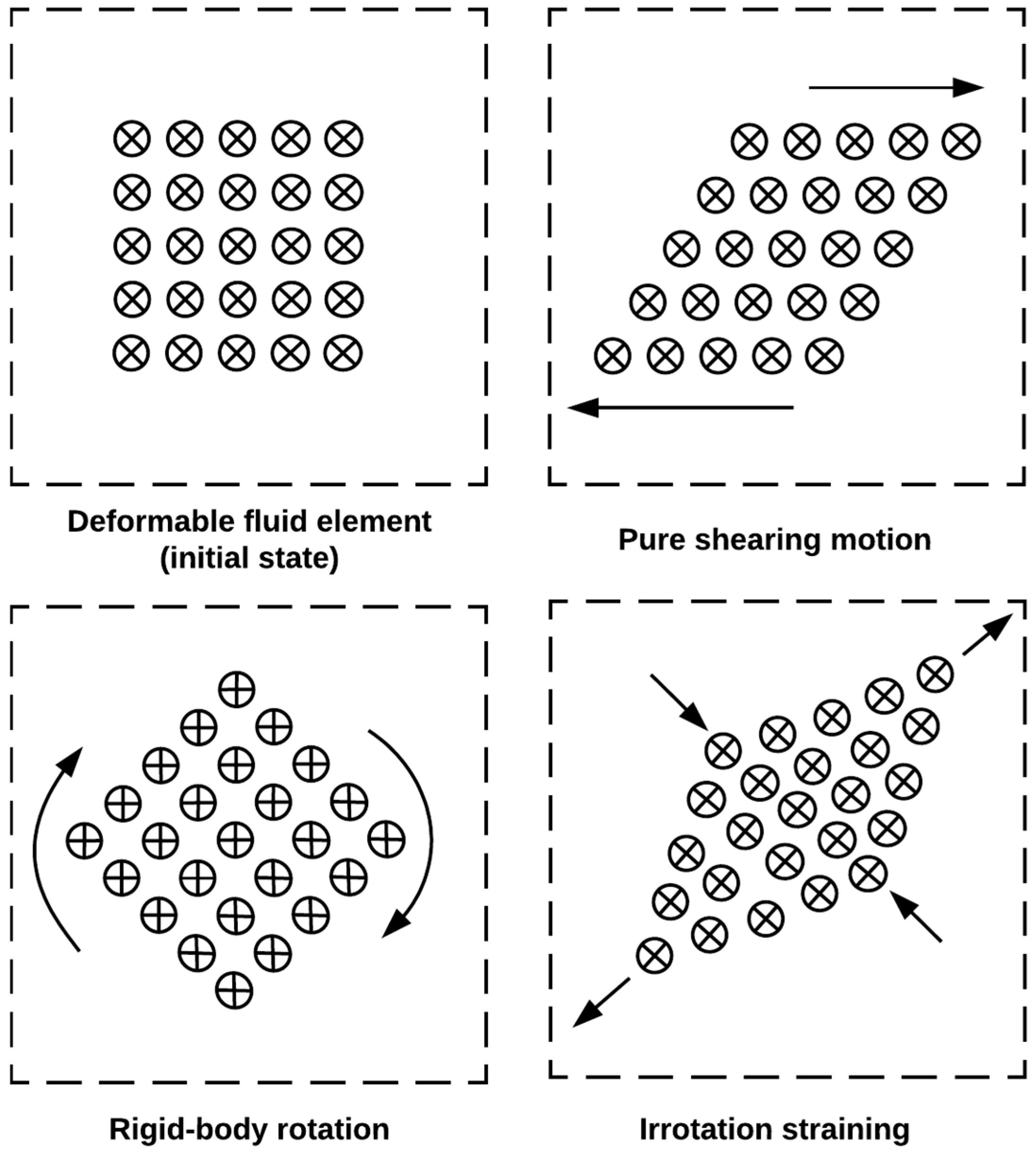
To solve this issue, Kolar introduced a method regarding the triple decomposition of the velocity gradient tensor, which distinguishes the pure shearing motion and actual swirling motion by decomposing the velocity gradient tensor [
29]. The aim is to decompose an arbitrary instantaneous state of the relative motion into three elementary motions. An illustration can be found in
Figure 6.
The velocity gradient tensor will be decomposed into three components to represent three elementary motions where the pure shearing should be purely asymmetric, the rigid-body rotation should be antisymmetric and the irrotational staining should be symmetric. The decomposition strategy is based on the characteristic of the motion and the matrix is decomposed into three parts. Equations (3)–(6) illustrate the process [
29]. The rigid-body rotation and irrotational straining are combined as the residential tensor.
The cyclone eye regions are characterized by the non-zero rotation tensor and
The identification output (the cyclone position in the grid index) will be stored in the cyclone database with PostGIS and used for the significant input of cyclone tracking. However, it still needs to be validated and estimated in the knowledge-driven system by comparing it with dynamic cyclone simulation and reanalysis data. Next, we give a brief introduction of the integration of identification output with real-time cyclone simulation.
4. Integrating Identification Output with Wind Simulation
Real-time wind simulation is the most intuitive and effective way to view cyclone activity. Like point clouds representing the surface of a 3D entity, large quantities of dynamic particles express physical phenomena effectively. By rendering massive unevenly distributed and animated particles, dynamic cyclone activities will be simulated and tracked from birth to death with the wind simulation submodule. Meanwhile, users can easily capture the dynamic cyclone by its appearance. Actually, the particle system has been widely used in experimental flow analysis. The integration of identification outcome with cyclone simulation enables us not only to validate the outcome but also to label the cyclone with a specific trajectory in the system. At this point, it is necessary to simulate the spatiotemporal wind field based on particle tracking in the web environment.
Particle tracing—which provides a Lagrange description of a problem by solving ordinary differential equations using Newton’s law of motion—provides an effective approach for field visualization. A geometric entity or phenomenon is represented by thousands of discrete and animated particles. The integration process in each rendering frame is briefly introduced below. The particle position is calculated and updated in each frame with the integral Equation (7).
p (t) and
p (t + ∆t) represent the particle position in time t and time t + ∆t. Further,
indicates the velocity and is determined by position and time. The 4D wind field data is compressed into a video using VP9 to solve the issue of data transmission from the remote server on web environment.
Resch et al. evaluate five different technologies on many criteria, such as web browser support, implementation complexity, and performance [
18]. WebGL is the best choice for us to visualize the wind data due to its characteristic of cross-platform and GPU (graphics processing unit) computing, enabling it to accelerate visualization [
30,
31]. To tessellate the wind data in a unified geometric frame, Cesium—an open-source JavaScript library for world-class 3D globes based on WebGL—is used for earth visualization [
32].
Figure 7 illustrates the process of one-frame rendering in our method. Three passes which are particle initialization, particle advection, and particle rendering are executed on the GPU in one-frame rendering.
Pass 1. Particle Initialization. Particle positions are initialized randomly and redistributed to emphasize the region of interest. The positions are stored in the RGB color components of a floating point texture along with particle lifetime in the alpha.
Pass 2. Particle Advection. The particle position is updated in each frame using the classical Euler scheme within the fragment shader in parallel. The wind vector from a random position used for moving the particle is accessed with the bi-linear interpolation on the GPU. A boundary test and death test need to be conducted to check if the particle should be recreated. Furthermore, a double frame buffer technique is used to avoid the write and read conflict. The output texture in particle advection is used for the input of particle rendering.
Pass 3. Particle Rendering. Once particle positions have been updated and fetched, the particles are rendered usually in the form of a texture billboard (pixel, oriented point spirits).
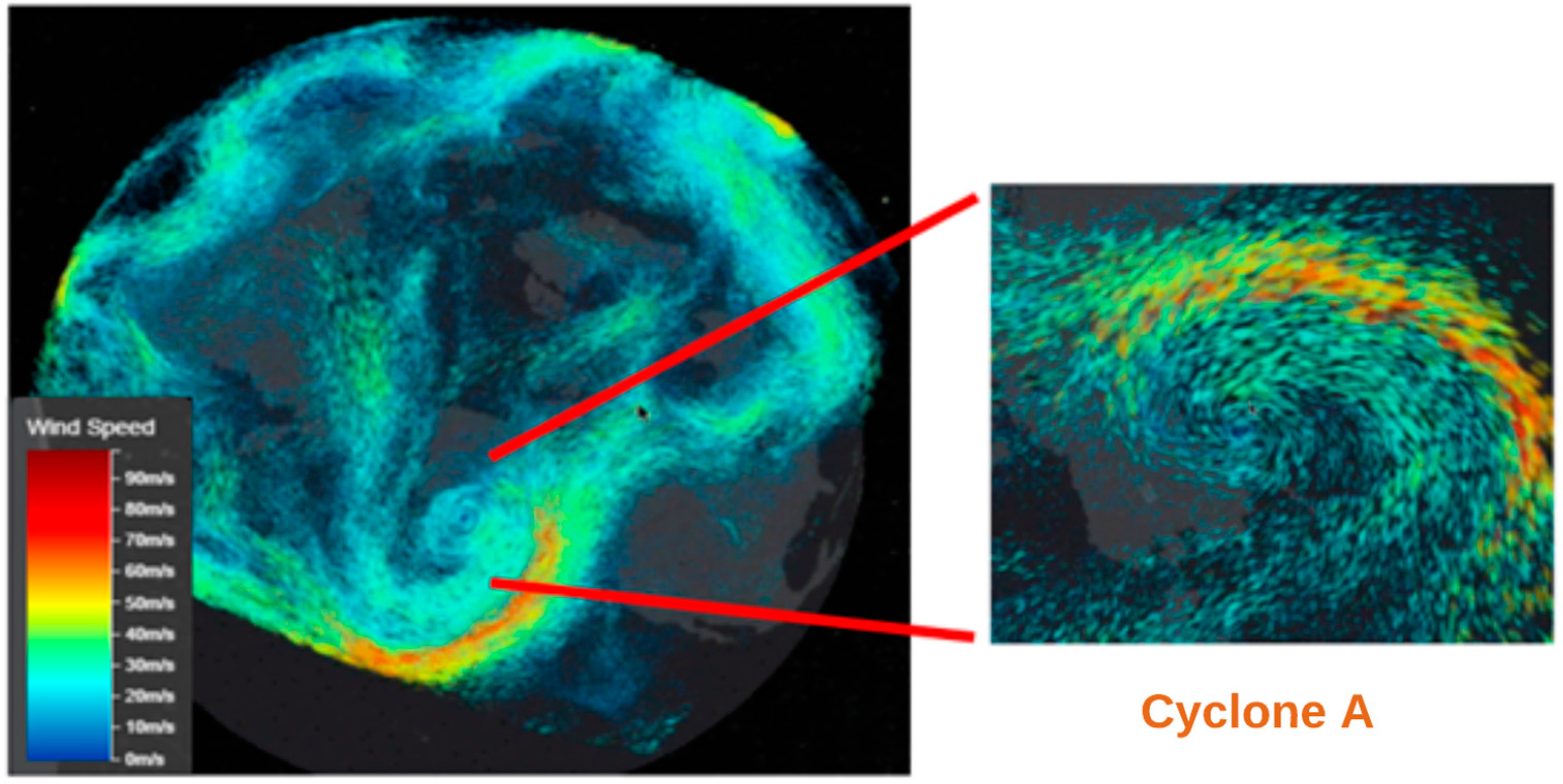
With the animation of particles, it is easy to visually distinguish and trace the vortex activity in the scenario (see cyclone A in
Figure 8). The cyclone identification outcome is rendered in each frame along with the simulation. The cyclone position is queried from the spatial database with the property of time and the user-defined selective rectangle. The integration of the identification outcome with cyclone simulation helps to validate the accuracy of the identification method mentioned in
Section 3. Meanwhile, it is a demonstration of how the cyclone extraction can be applied to real applications. The spatiotemporal query enables the user to focus on the interested cyclone within a specific time and space.
6. Conclusions
Driven by helping scientists discover knowledge from raw atmospheric data around the North Pole, a cyclone identification approach is proposed to extract and track cyclones from spatiotemporal wind data in this paper. A combination of pressure minima criteria and velocity filter criteria is exploited to reduce the limitation of the existing criteria. The accuracy of the cyclone identification is demonstrated by comparing the identification result with the plotted figure and NCEP/NCAR reanalysis data using eight groups of data captured in 2007. The statistical results show that the proposed approach can effectively identify the complicated cyclones in the North Pole with an accuracy of over 95%. Based on this approach, a web-based knowledge-driven and decision-making system is architected where the 4D wind simulation is based on particle tracking.
Furthermore, by introducing the cyclone identification concept and method in the North Pole, this paper aims at facilitating atmospheric activity detection research on massive spatiotemporal climate data. The present framework should still be considered to be a work in progress and further work should be focused on real-time cyclone identification and performance optimization.
In the future, more work will be conducted on the automated activity detection technology and abstract identification method to extract variable atmospheric events. The detailed discussion should be taken over on the atmospheric phenomenon definition and universal detection scheme. Additionally, atmospheric event identification with Artificial Intelligence (AI) is another direction to be studied.


