3.1. Model Performance Evaluation
The local meteorological patterns affect the transport, transmission, advection, and diffusion of pollutants over the regional scale and further continental scales, which cannot be fully captured by the model to some extent [
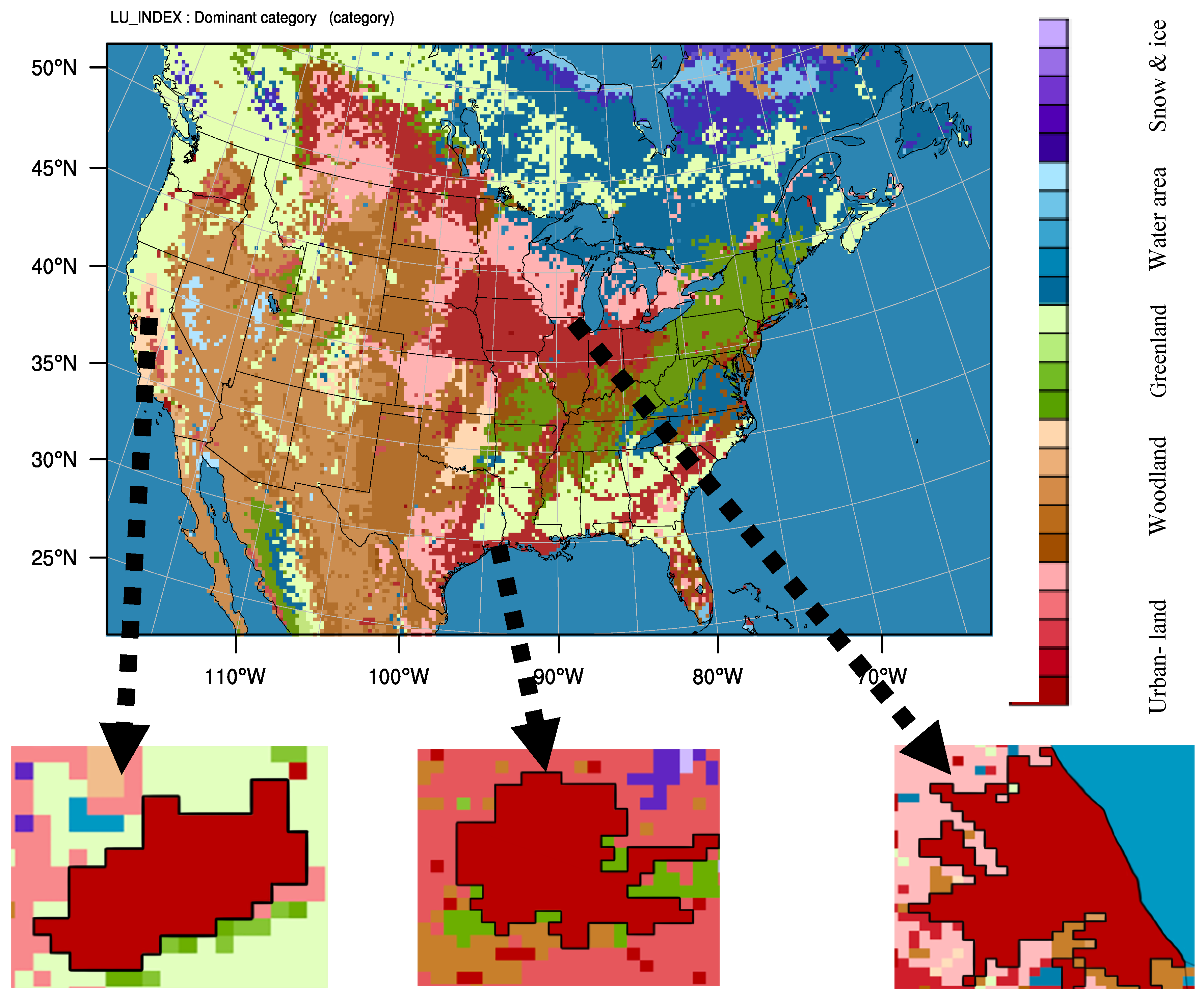
18]. We evaluated the model performance of WRF_ChemV3.6.1 by comparing the simulation results with observations obtained from weather and air-quality stations in Sacramento, Houston, and Chicago. The weather and air quality monitoring stations were chosen based on their locations close to the downtown of the selected cities (hereafter referred to as urban) and their surroundings (hereafter referred to as suburb). The hourly 2-m air temperature (T2), 10-m wind speed (WS10), 2-m relative humidity (RH2), and dew point temperature (Td) simulation results are compared with the measurements obtained from the U.S. Environmental Protection Agency (EPA) Clean Air Status and Trend Network (CASTNET). The daily averaged modelled fine particular matters (PM
2.5), ozone (O
3), nitrogen dioxide (NO
2), PM
2.5 subspecies (particulate sulfate (SO4
2.5), particulate nitrate (NO3
2.5), and organic carbon (OC
2.5)) concentrations are compared with the EPA Air Quality System (AQS) observations using 24-h average data. [
45,
46,
47,
48,
49]
Here, the time series of simulation results changed to the local time for each specific location: Sacramento: LST = UTC − 7 h; Houston and Chicago: LST = UTC − 5 h. The performance and accuracy of the simulation results are quantitatively based on a series of metrics estimations [
50]. Here, we followed the Zhang et al. [
51] calculations for the mean bias error (MBE), mean absolute error (MAE), and the root mean square error (RMSE) estimations of the meteorological and chemical parameters.
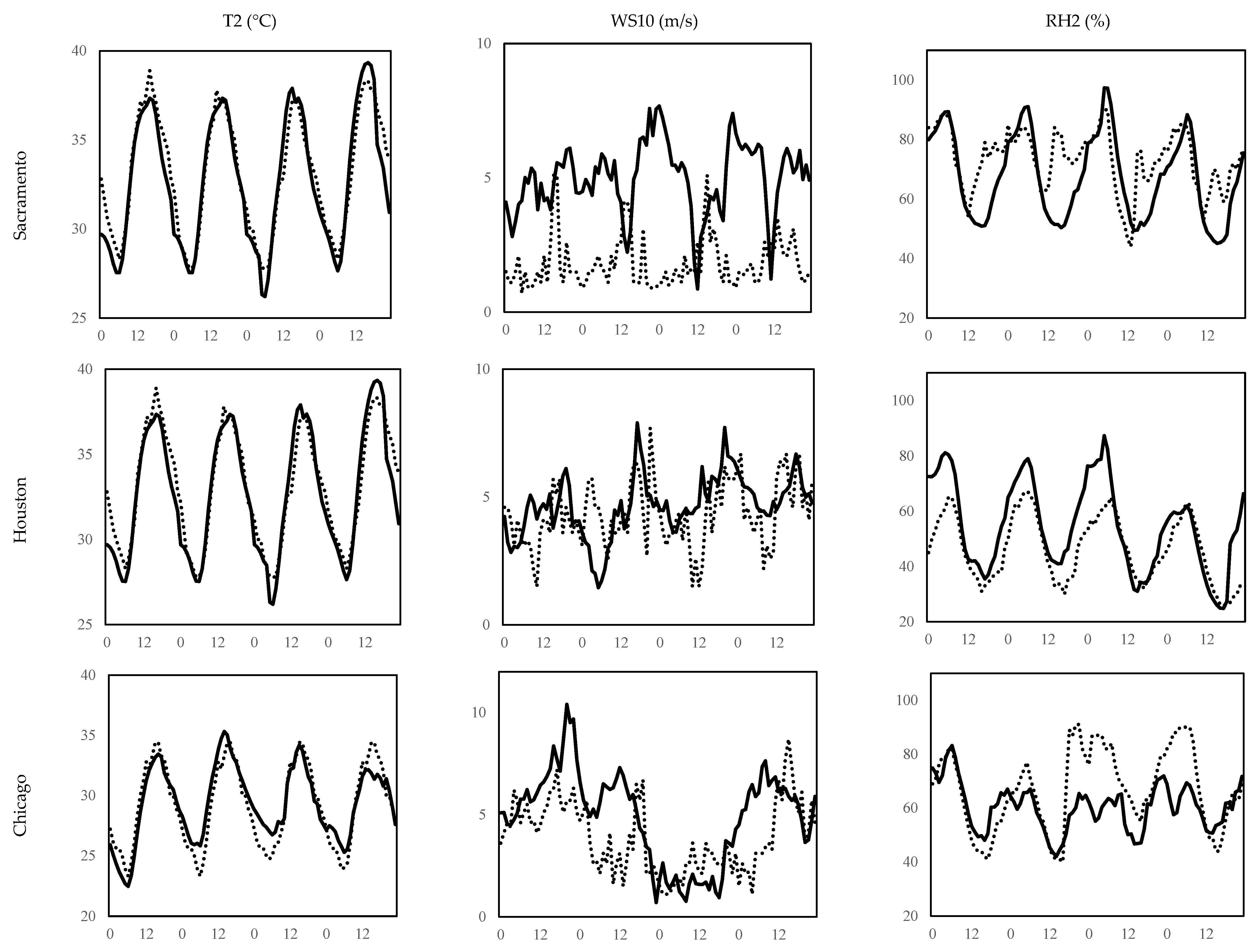
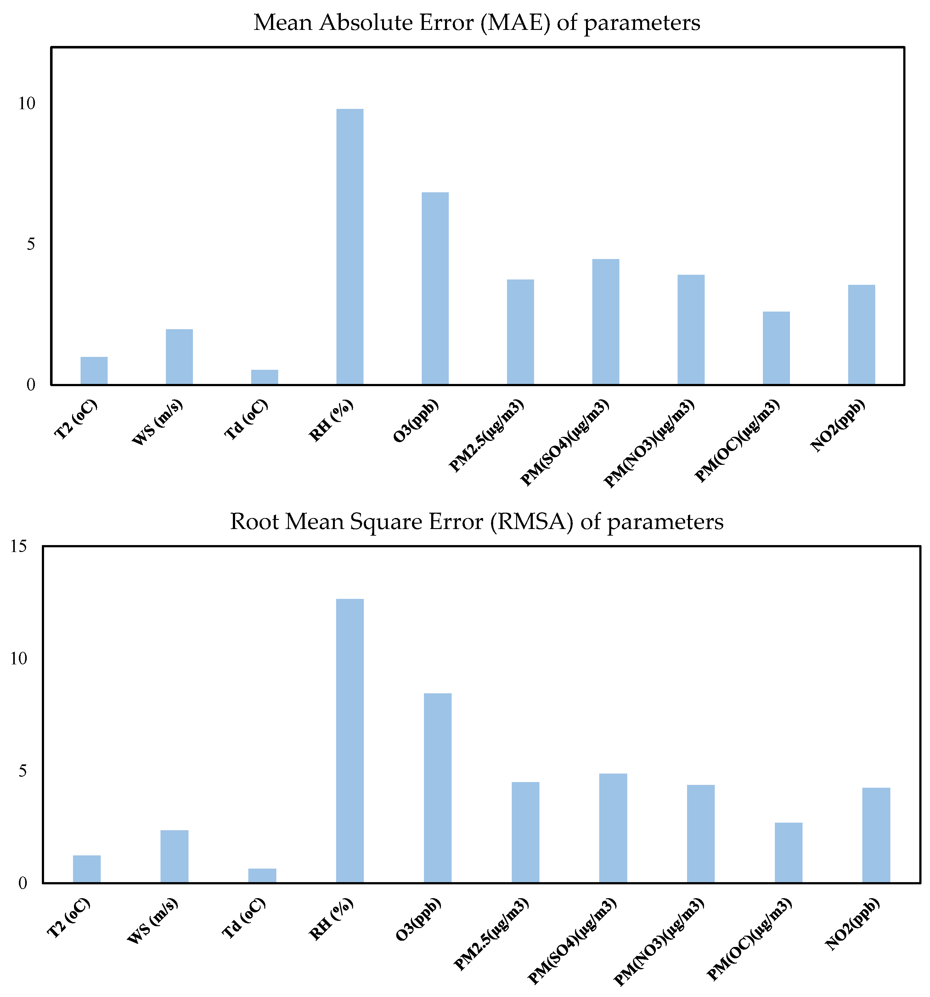
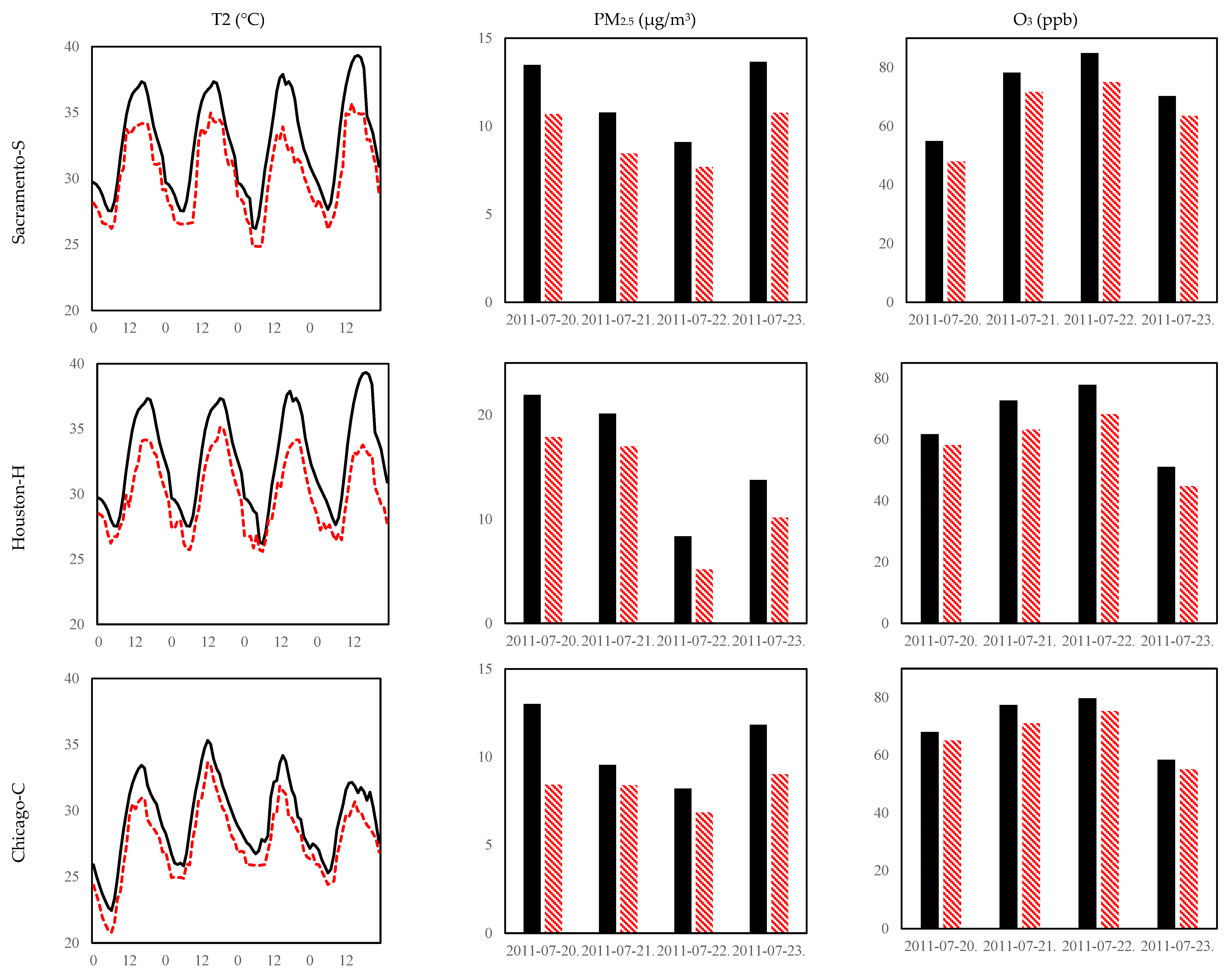
In terms of meteorological components of the model, the WRF-ChemV3.6.1 effectively captures the diurnal variations of 2-m air temperature, overpredicts 10-m wind speed, overpredicts dew point temperature, and underpredicts 2-m relative humidity. The MBA of T2 (−0.07 °C) shows that the model is capable in predicting air temperature. A small underprediction can be seen in urban areas (~−0.3 °C) that indicates the model deficiency in calculating the heat emission from anthropogenic sources in urban areas accurately. The MAE and RMSE of T2 are approximately 1 °C. Wind speed plays an important role in calculation of air temperature from skin temperature in the land surface model. The 10-m wind speed comparisons show small to large overpredictions (0.3 to 3.15 m/s). The MBA is 1.65 m/s, that shows the model is unable to capture the effects of micro scales and wind patterns. The MAE and RMSE of WS10 are almost 2 m/s. Relative humidity is a function of moisture content, air temperature, and surface pressure. The spatial distribution of RH2 represents an underestimation with the MBE of −1.42%. This underestimation shows that the microphysics scheme miscalculated the processes of transforming water (rain, vapor, cloud, etc.) and moisture fluxes. It also shows the model limitation in capturing the sea surface temperature, wind speed, and their impacts on water mixing ratio and water content of the air properly. The MAE and RMSE of RH2 are nearly 10% and 13%, respectively.
Figure 2 shows the time series (hourly) of the observed vs. simulated T2 (°C), WS10 (m/s), and RH2 (%) in the urban areas of Sacramento, Houston, and Chicago. We also calculated the dew point temperature to avoid the dependency on air temperature for the moisture variable. The MBA, MAE, and RMSE of dew point temperature (0.39, 0.53, and 0.65 °C, respectively) show that the model overpredicts the moisture content in the atmosphere especially in urban areas (~0.5 °C).
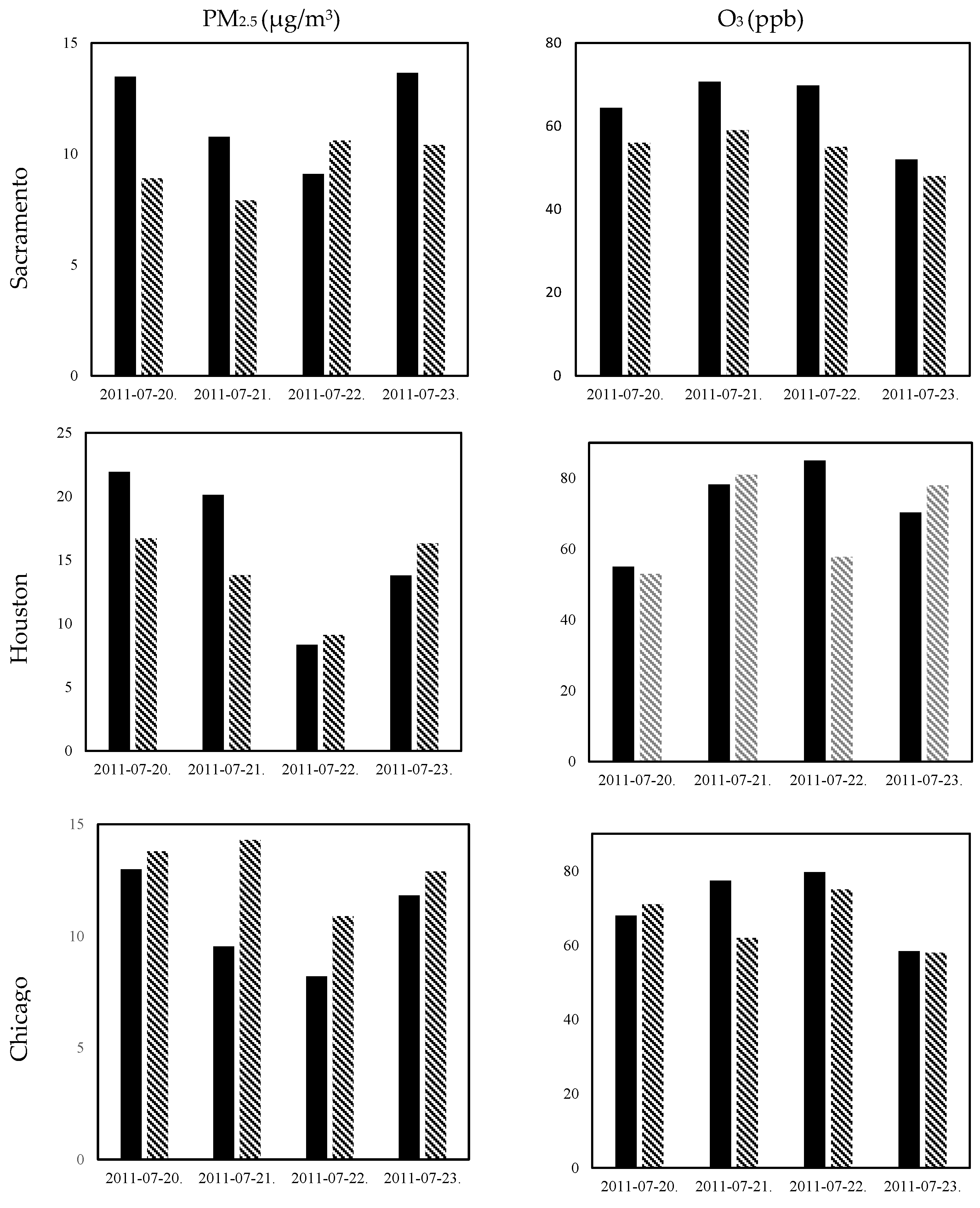
In terms of the chemical component of the model, the WRF_ChemV3.6.1, as configured here, tends to underpredict 24-h fine particular matters (PM2.5) and over-predict the 24-h O3 concentrations during the 2011 heat wave period. The MBE of the 24-h avg. PM2.5 is −1.42 µg/m3. The MAE and RMSE of PM2.5 are approximately 4 µg/m3. This is because the accuracy in fine particular matters concentrations is to some extent a function of its subspecies estimations as particulate sulfate, particulate nitrate, and organic carbons. Thus, we also compared the simulation results of SO42.5 (µg/m3), NO32.5 (µg/m3), and OC2.5 (µg/m3) with observations at urban areas of aforementioned cities. We observed that the performance of PM2.5 subspecies is a combination of overprediction of particulate sulfate (MBE ~ 5 µg/m3) and underprediction of particulate nitrate (MBE ~ −4 µg/m3) and organic carbon (MBE ~ −3 µg/m3). The MAE and RMSE of SO42.5, NO32.5, and OC2.5 are approximately 5, 4, and 3 µg/m3, respectively. The comparison between simulated ozone and measurements indicated an overestimation of O3 across the domains (MBE ~ 5 ppb). The O3 concentrations is overestimated due to the NOx and VOCs overestimation in emission inventories and their calculations in chemistry packages (US-NEI11 and MEGAN). The average MAE and RMSE of O3 are around 7 ppb and 8 ppb, respectively. We also calculated the NO2 concentrations as one of the precursor in ozone formation. The MBE of NO2 in urban areas (~2.5 ppb) show that the model tends to overpredict the nitrogen dioxide. The MAE and RMSE of NO2 is around 4 ppb.
Figure 3 shows the observed vs. simulated PM
2.5 (µg/m
3) and O
3 (ppb) concentrations in the urban areas of Sacramento, Houston, and Chicago.
Table 3,
Table 4 and
Table 5 respectively represent the mean bias error (MBE), mean absolute error (MAE), and the root mean square error (RMSE) of T2 (°C), WS10 (m/s), RH2 (%), PM
2.5 (µg/m
3), and O
3 (ppb) for aforementioned cities. There are several limitations and assumptions in these comparisons. The simulation results are extracted hourly for all variables, whereas the observation in terms of PM
2.5 and O
3 are reported as a 24-h average.
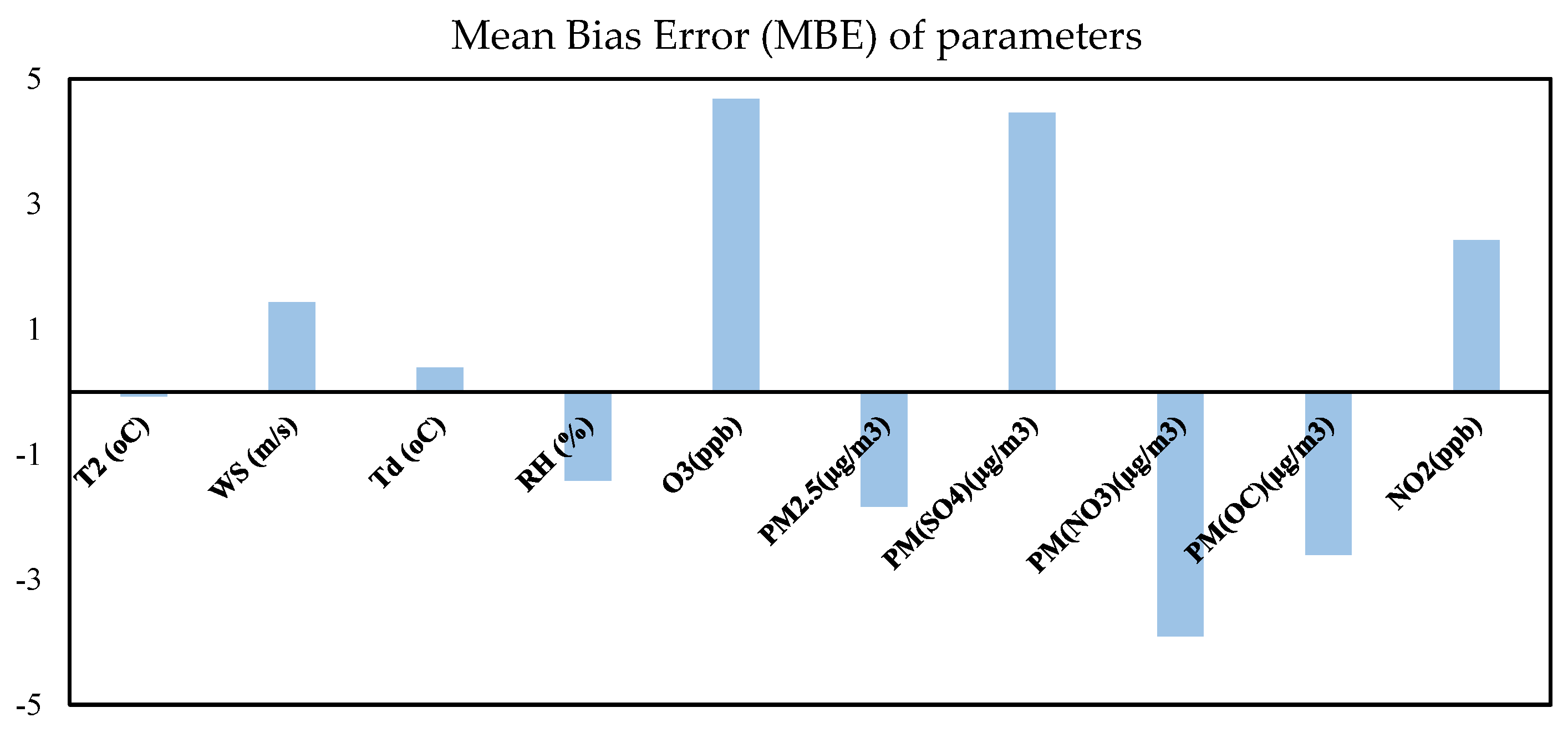
Figure 4 shows the overall comparison between observed vs. simulated aforementioned parameters in terms of MBA, MAE, and RMSE. Despite the model biases in simulating meteorological and chemical variables, the performance of WRF-ChemV3.6.1 is generally consistent with most air quality models. For comparison of thermal components, the fifth-generation NCAR/Penn State Mesoscale Model (MM5) presented the MBE of T2 as 0.4 °C to −3.8 °C during a year [
52,
53,
54,
55]. For comparison of chemical components, the CMAQ model was run during a year and indicated an under estimation of PM
2.5 as the MBE of −0.6 µg/m
3 and an overprediction of seasonal O
3 as the MBE of 4.4 ppb [
56]. However, given the various differences in physical and chemical parameterizations and input data (different simulation year and observations), the online coupled WRF-Chem is mostly suited for application of simulating and investigating the effects of urban heat island and its mitigation strategies.
3.2. Effects of Increasing Urban Albedo
Results discussed here are based on the comparison between the ALBEDO and CTRL scenarios for each city.
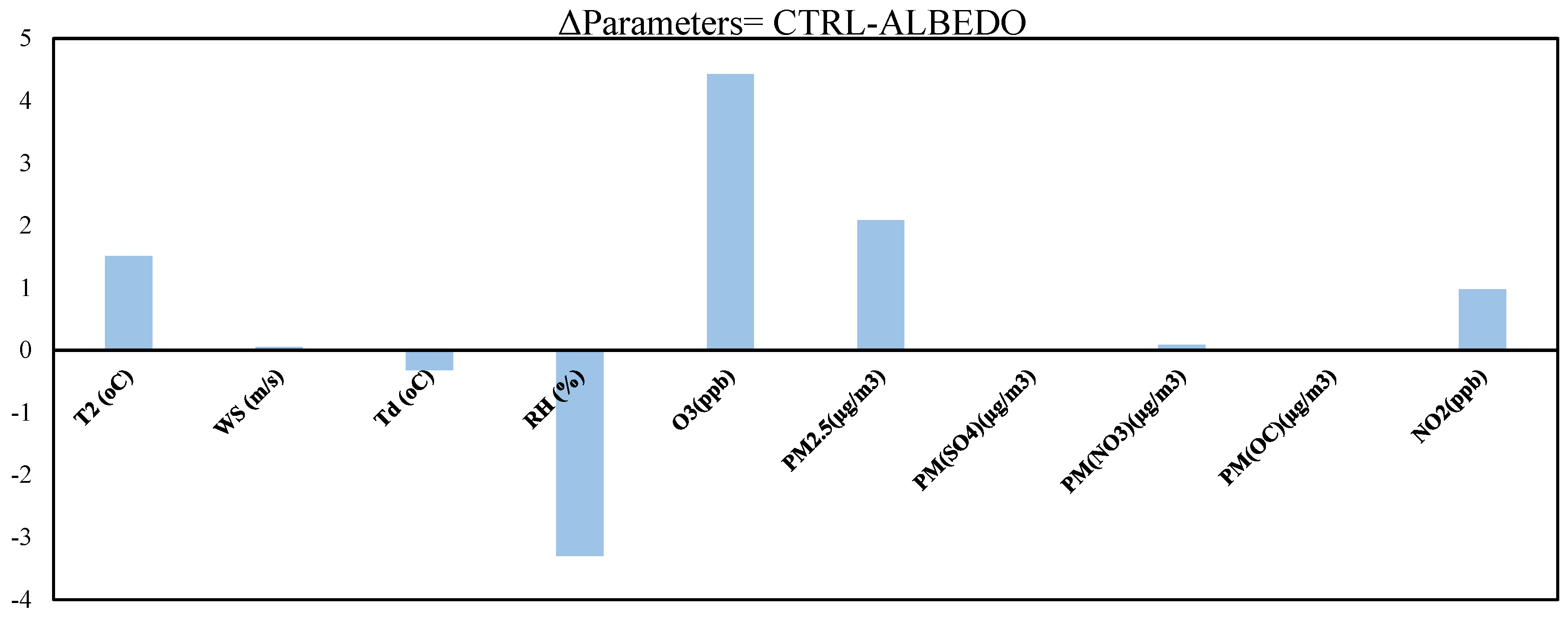
Table 6 and
Figure 5 represent the average differences in T2 (°C), WS10 (m/s), Td (°C), RH2 (%), PM
2.5 (µg/m
3), O
3 (ppb), SO4
2.5 (µg/m
3), NO3
2.5 (µg/m
3), OC
2.5 (µg/m
3), and NO
2 (ppb) during the 2011 heat wave period across the second, third, and fourth domains: Sacramento (CA), Houston (TX), and Chicago (IL).
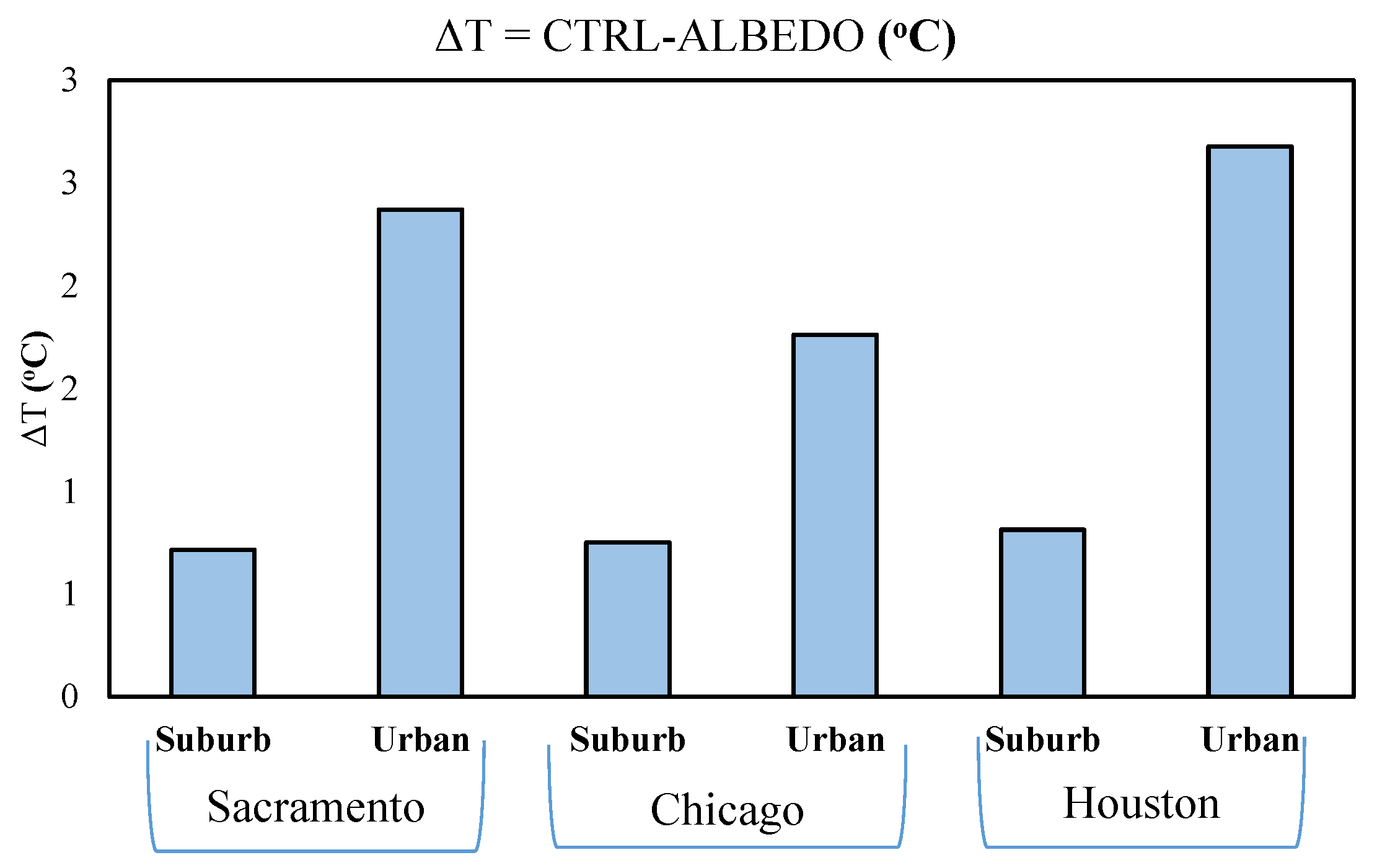
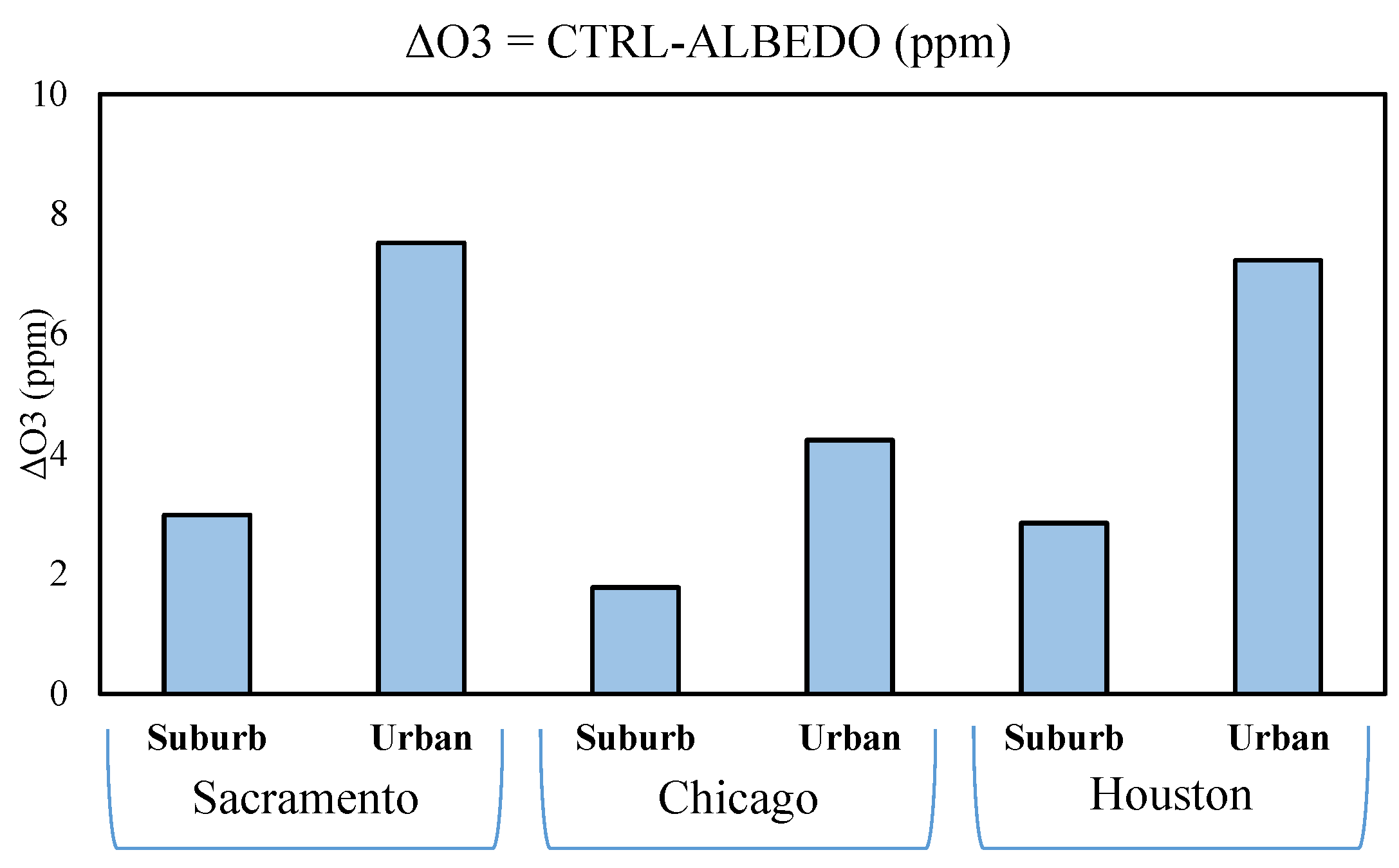
Figure 6 shows the averaged differences of T2 (°C) and O
3 (ppb) concentrations in suburb and urban areas of the aforementioned cities.
Sacramento, California is located in the central valley near the Sierra foothills. It is at the confluence of the Sacramento River and the American River and is known as the Sacramento Valley. The city has a population of approximately 500,000 people and covers over 253 km
2 [
57,
58]. Its climate is characterized by mild year-round temperature. It has a hot-dry-summer Mediterranean climate with little humidity and an abundance of sunshine. Based on the National Oceanic and Atmospheric Administration (NOAA) Online Weather Data [
22], Sacramento has the summer temperature exceeding 32 °C on 73 days and 38 °C on 15 days. The State of the Air 2017 report, by American Lung Association [
59], ranks the metropolitan areas based on ozone and particular pollutions during 2013, 2014, and 2015 period. They used the official data from the U.S. Environmental Protection Agency (EPA). Sacramento ranks eighth because of its high ozone concentration.
In a study performed at the Lawrence Berkeley National Laboratory (LBNL), Taha et al. [
60] applied the Colorado State Urban Meteorological Model (CSUMM) and the Urban Airshed Model (UAM-IV) to estimate the impacts of heat island mitigation strategies in Sacramento on the area’s local meteorology and ozone air quality in 2000. The albedo level and vegetative cover increased by approximately 0.11 and 0.14, respectively. Using 11–13 July 1990 as the modeling period, the ozone and temperature decreased by up to 10 ppb and 1.6 °C, respectively. In a more recent study, Taha et al. [
61] applied WRF with CMAQ in Sacramento Valley with the inner domain of 1 km resolution. The albedo of roofs, walls, and pavements increased by 0.4, 0.1, and 0.2, respectively. The surface temperature and air temperature were reduced by up to 7 °C and 2–3 °C, respectively. The ozone concentrations also decreased by up to 5–11 ppb during the daytime.
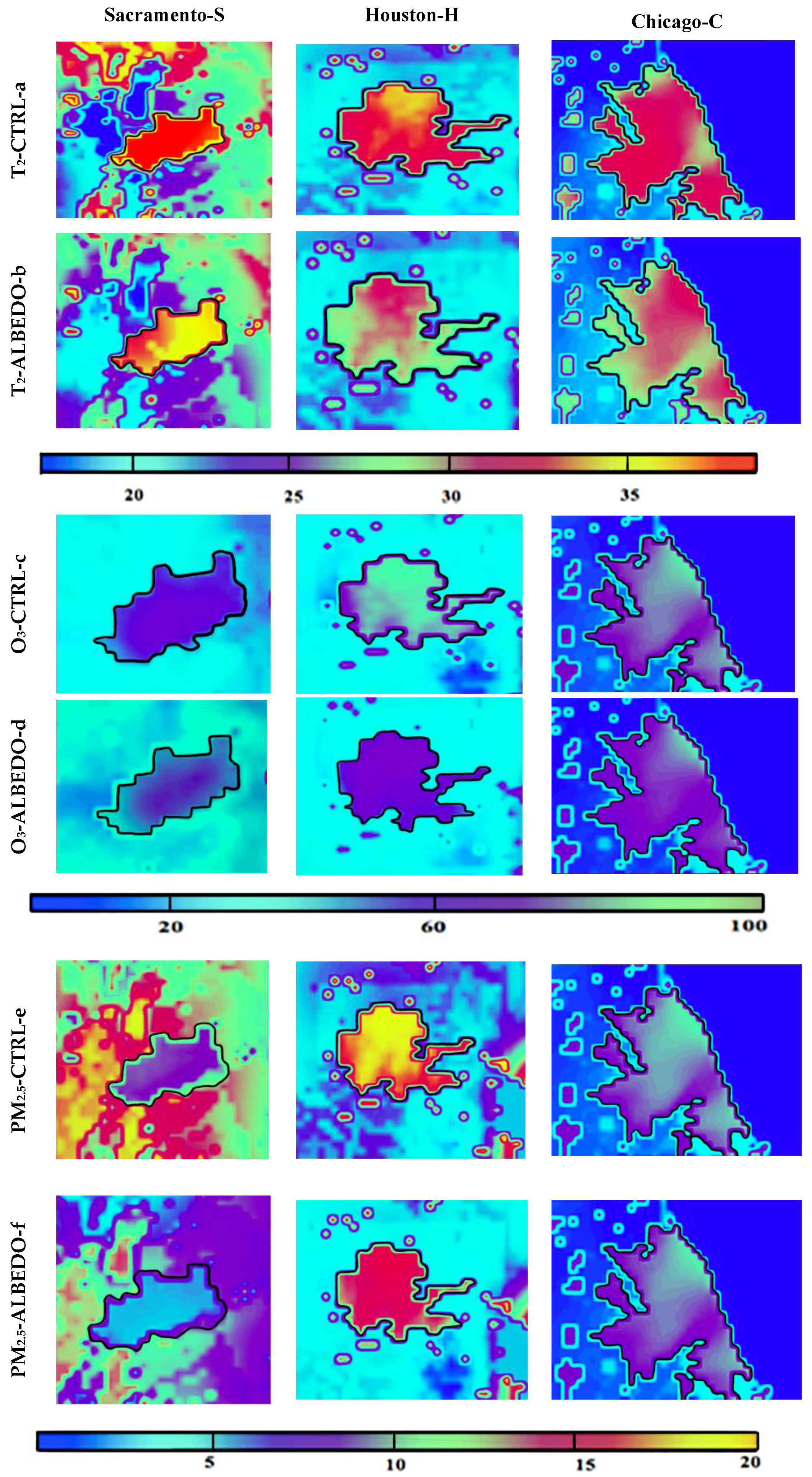
Our simulation results for Sacramento show that albedo enhancement leads to a net decrease in 2-m air temperature by up to 2.5 °C and 0.7 °C in urban and suburban areas, respectively. Most of the decreases occur between 1200 and 1600 LST as shown in
Figure 7-S.
Figure 8-Sa (CTRL) shows the maximum air temperature across the simulation domain in the heat wave period. By increasing surface reflectivity, the maximum temperature reduction is around 3 °C almost in all parts of the city (
Figure 8-Sb-ALBEDO) and this reduction is more obvious in the western part of the domain. The wind speed slightly decreased over the entire domain. The relative humidity increased by 7% and 3% in urban and suburban areas, respectively. Increasing surface reflectivity affords a decrease of nearly 2.4 µg/m
3 in PM
2.5 concentrations in urban area (
Figure 7-S) and 1 µg/m
3 in suburb.
Figure 8-Sc shows the maximum PM
2.5 concentrations across the domain. The maximum is around 12 µg/m
3 in urban area that decreases by 2–3 µg/m
3 as the results of albedo enhancement (
Figure 8-Sd). The heat island mitigation strategy causes a decline in O
3 by almost 8 ppb in urban (
Figure 7-S) and 3 ppb in suburb of the Sacramento area.
Figure 8-Se shows the maximum O
3 concentrations as nearly 80 ppb across the simulation domain that decreases to nearly 70 ppb by UHI mitigation strategy (
Figure 8-Sf). Our results resemble those of previous studies [
60,
61,
62,
63]. We have also compared the CTRL and ALBEDO simulations results of particulate sulfate, particulate nitrate, organic carbon, and nitrogen dioxide. Albedo enhancement causes no changes (OC) to minimal changes to particular matters subspecies (~0.01 reduction) but decreases the NO
2 concentration by 0.82 ppb.
Houston is the fourth most populous city in the U.S. with a population of 2.3 million within a land area of 1700 km
2 [
57,
58]. It is located in the Southeast Texas near the Gulf of Mexico. Houston’s climate is classified as humid subtropical. During the summer, the temperature commonly reaches 34 °C, and some days it reaches to even 40 °C. The wind comes from the south and southeast and brings heat and moisture from the Gulf of Mexico. The highest temperature recorded in Houston is 43 °C, which occurred during the 2011 heat wave period [
57,
58]. Houston also suffers from excessive ozone levels and the American Lung Association [
59] named the city as the 12th most polluted city in the U.S., based on EPA 2013, 2014, and 2015 data base.
Taha [
64] used MM5 to evaluate the model’s episode performance and its response to increasing surface albedo and vegetation in Houston during several days in August 2000. In ALBEDO scenario, the roof albedo was increased from an average of 0.1 to an average of 0.3; wall albedo was increased from an average of 0.25 to an average of 0.3; pavement albedo was increased from an average of 0.08 to 0.2. The results indicated a reduction in temperature by up to 3.5 °C, and also caused warming in some areas by up to 1.5 °C. Results indicated that cooling usually occurs during daytime, while heating occurs at night. The other simulations show the same results [
64,
65,
66].
Our simulation results for Houston show that albedo enhancement leads to a net decrease in 2-m air temperature by up to 3 °C and 0.8 °C in urban (
Figure 7-H) and suburban areas, respectively. We witness no heating effect in our simulation. The reason is due to the sea breeze consideration in the solver of WRF-Chem.
Figure 8-Ha illustrates the maximum air temperature across the Houston in the heat wave period. The maximum temperature reduction is above 3 °C almost in all parts of the city (
Figure 8-Hb). Our model tends to perform relatively better in urban rather than in suburb areas. With albedo enhancement, the wind speed slightly decreased, and the relative humidity increased by up to 7% in urban and 3% in suburb. Increasing surface reflectivity affords a decrease of PM
2.5 concentrations by up to 3.5 µg/m
3 and 2.6 µg/m
3 in urban and suburban areas, respectively.
Figure 8-Hc shows the maximum PM
2.5 concentrations across Houston. The maximum is above 20 µg/m
3 in urban area that decreases to 16 µg/m
3 as the results of albedo enhancement (
Figure 8-Hd). The O
3 concentrations also decrease by up to 7.2 ppb and 3 ppb in urban and suburban areas, respectively.
Figure 8-He shows the maximum O
3 concentrations as above 80 ppb across the simulation domain that decreases to nearly 70 ppb all over the domain (
Figure 8-Hf). Our results resemble to previous studies [
64,
65,
66]. Increasing surface albedo in the urban area of Houston causes no changes in particular matters subspecies and a decrease of 1.2 ppb in NO
2 concentration.
Chicago is the third most populous city in the U.S. with over 2.7 million residents. The city area is 606 km
2 [
57,
58]. The city lies on the southwestern shores of Lake Michigan and has two rivers: the Chicago River and the Calumet River. Chicago has a humid continental climate. Summer temperatures can reach up to 32 °C. Taha et al. [
67] used a three-dimensional, Eulerian, mesoscale meteorological model (CSUMM) to simulate the effects of large scale surface modifications on meteorological conditions in 10 cities across the U.S. Surface modifications included increasing albedo by 0.03 ± 0.05 and increasing vegetative fraction by 0.03 ± 0.04. The results indicated that the air temperature was reduced by up to 1 °C in the Chicago area.
Our simulation results for Chicago show that albedo enhancement leads to a net decrease in 2-m air temperature by up to nearly 2 °C and 0.8 °C in urban (
Figure 7-C) and suburban areas, respectively.
Figure 8-Ca shows the maximum air temperature across the simulation domain. With albedo enhancement, the air temperature reduced over the domain (
Figure 8-Cb). The wind speed slightly reduces in suburbs, with no changes in urban areas. The results show a slight decrease in relative humidity by up to 0.2% in Chicago’s urban areas. The reason is due to the wind speed direction that is north to west (passing the bodies of water) and the city’s location that is along one of the Great Lakes, Lake Michigan, and has the Mississippi River Watershed and the Chicago River. The other reason is due to the increasing surface reflectivity that reduces the skin temperature and thus air temperature that might also decrease the chance of evaporation and thus decreases moisture content above the ground. This strategy also affords a decrease of PM
2.5 concentrations by up to 2.5 µg/m
3 and 0.6 µg/m
3 in urban and suburban areas, respectively. The maximum PM
2.5 concentrations across Chicago is nearly 12 µg/m
3, that decreases to nearly 9 µg/m
3 as the results of albedo enhancement (
Figure 8-Cc and Cd). The O
3 concentrations decrease by up to 4.2 ppb in urban area and 1.7 ppb in suburb.
Figure 8-Ce shows the maximum O
3 concentrations as nearly 70 ppb across the simulation domain that decreases to almost 65 ppb all over the domain (
Figure 8-Cf). Increasing urban albedo in Chicago leads to an increase of particulate nitrate by 3 ppb and a decrease of NO
2 concentration by 0.9 ppb.
Overall, the results indicate that with albedo enhancement, the air temperature drops (~1.5 °C) and thus causes a decrease in ozone concentrations (~5 ppb) and nitrogen dioxide (~1 ppb). Increasing surface solar reflectance lead to a minimal decrease in particular matters (~2 µg/m3) and no significant changes in its subspecies. The SO42.5 and NO32.5 concentrations reduced slightly in urban areas (~0.1 µg/m3) due to the decrease in air temperature and thus photochemical reaction rates, but there is no change in OC2.5 (µg/m3). The UHI mitigation strategy increased the relative humidity and dew point temperature. Our results show that there are no significant changes in the wind speed over the domain and the differences between two scenarios is 0.05 m/s. This minimal change can be due to the WRF-Chem configurations and it does not reflect any changes in momentum transport from the shallow boundary layer.


