Abstract
The impact of climate and land use/land cover (LULC) change continues to threaten water resources availability for the agriculturally used inland valley wetlands and their catchments in East Africa. This study assessed climate and LULC change impacts on the hydrological processes of a tropical headwater inland valley catchment in Uganda. The hydrological model Soil and Water Assessment Tool (SWAT) was applied to analyze climate and LULC change impacts on the hydrological processes. An ensemble of six regional climate models (RCMs) from the Coordinated Regional Downscaling Experiment for two Representative Concentration Pathways (RCPs), RCP4.5 and RCP8.5, were used for climate change assessment for historical (1976–2005) and future climate (2021–2050). Four LULC scenarios defined as exploitation, total conservation, slope conservation, and protection of headwater catchment were considered. The results indicate an increase in precipitation by 7.4% and 21.8% of the annual averages in the future under RCP4.5 and RCP8.5, respectively. Future wet conditions are more pronounced in the short rainy season than in the long rainy season. Flooding intensity is likely to increase during the rainy season with low flows more pronounced in the dry season. Increases in future annual averages of water yield (29.0% and 42.7% under RCP4.5 and RCP8.5, respectively) and surface runoff (37.6% and 51.8% under RCP4.5 and RCP8.5, respectively) relative to the historical simulations are projected. LULC and climate change individually will cause changes in the inland valley hydrological processes, but more pronounced changes are expected if the drivers are combined, although LULC changes will have a dominant influence. Adoption of total conservation, slope conservation and protection of headwater catchment LULC scenarios will significantly reduce climate change impacts on water resources in the inland valley. Thus, if sustainable climate-smart management practices are adopted, the availability of water resources for human consumption and agricultural production will increase.
1. Introduction
The impacts of climate change such as rising temperatures and unpredictable precipitation intensity and patterns have become undeniably unequivocal in East Africa [1,2,3], impacting the fragile ecosystems such as wetlands in the region. In addition, human and environmental stressors such as land use changes associated with rapid urbanization and uncoordinated expansion of intensive agricultural production in these wetlands negatively impair their water availability, quality and other ecosystem services and functioning [2,4,5]. The negative impacts associated with climate and land use change are also compounded by other factors, notably exacerbating poverty and high population pressure, which is anticipated to increase demand for food and water in the future [6,7].
Wetlands cover 30,105 km2 of Uganda’s total land area of 241,500 km2, a share of 13% of the total land area [8], representing one of the most vital ecological and economic resources in the country. Wetlands offer numerous ecosystem services and functions ranging from provisioning to regulation and cultural services [9,10,11,12]. However, their integrity in offering ecosystem services and functions are being jeopardized due to factors such as anthropogenic activities, including population growth, degradation of arable upland soils, and increasing unpredictability of precipitation [13,14]. In fact, a decline in 26% of total wetland coverage in the Lake Kyoga basin and 53.8% in the Lake Victoria basin in Uganda have been reported [8]. Inland valleys are the most affected wetland types and are seen to possess a huge potential for agricultural production due to their soil water availability throughout the year and the inherent soil fertility [15,16,17,18], which encourage continuous agricultural production. Inland valleys are highly diverse and complex systems of variable ecosystems from the upland areas through the hydromorphic fringe to the valley bottom, with each valley being characterized by a typical hydrology [19,20]. Inland valleys are extensively distributed and seasonally flooded with noticeable impacts on the catchment hydrology [21]. The increased conversion of pristine inland valley wetlands into agricultural sites possesses significant threats to water resources, more so amidst the ubiquitous future climate change. Water resources will be tremendously altered as global climate models (GCMs) and regional climate models (RCMs) project an increase in mean temperature of 1.7–5.4 °C and precipitation of 5–20% by the end of the 21st century in East Africa [22,23,24]. There is high rainfall variability over the East African region with the northern part of the region receiving rainfall from June to September (JJAS) and the equatorial part of the region experiencing bimodal rainfall seasons in the year with the so-called ‘long rains’ occurring during March to May (MAM) and ‘short rains’ from September to November (SON) [25]. Most parts of eastern Africa have experienced frequent droughts and a decline in total rainfall during the long rains [26,27], although GCM projections show wetter conditions in the future [27], a contradiction which has been referred to as the East African paradox by Rowell et al. [26]. In fact, the Intergovernmental Panel on Climate Change (IPCC) Fifth Assessment Report (AR5) reports large levels of uncertainty in the temporal and spatial variability of precipitation over East Africa in the future [5]. According to Endris et al. [25], the GCM and RCM data project a decrease in seasonal rainfall over most parts of East Africa during the June to September (JJAS) and March to May (MAM) seasons. While an increase in rainfall over equatorial and southern parts of the region during the October to December (OND) season is projected, with higher changes in the equatorial region.
Given that wetlands are highly vulnerable to changes in the quantity and quality of their water supply, climate change coupled with the ongoing land use alterations will significantly affect the ecological attributes of these wetlands. Moreover, the loss of wetlands could exacerbate the impact of climate change since they provide fundamental services that contribute to mitigation of such impacts. Thus, a better understanding of the interacting impacts of climate and land use management changes on hydrological processes in these wetlands is crucial for sustainable agricultural development and water resources management.
There exist limited studies [28,29,30,31,32] that have demonstrated the impact of climate and land use change on the hydrological processes in the wetland–catchment nexus in East Africa. Yet, this information is vital to evaluate the possible vulnerability and resilience of these ecosystems to climate change, in particular the impacts of low predictability of precipitation. Hydrological modelling coupled with climate change and land use change scenarios enables the assessment of potential impacts of climate and land use change on water resources for well-informed decision making on the wise use of these ecosystems. Therefore, this study aims to assess the potential impacts of climate change and land use management on the water resources of an agriculturally used inland valley in Central Uganda using the Soil and Water Assessment Tool (SWAT). Specifically, the study analyzes (1) the impact of climate change on the hydrological processes within the inland valley and (2) which land use management scenarios may alleviate the negative effects of climate change on water resources of the inland valley. The projected results are envisaged to provide supporting scientific information for decision making, sustainable planning, agricultural production, and water resources management at the local scale in the inland valleys of the country and the surrounding region under changing climate and land use.
2. Materials and Methods
2.1. Description of Study Area
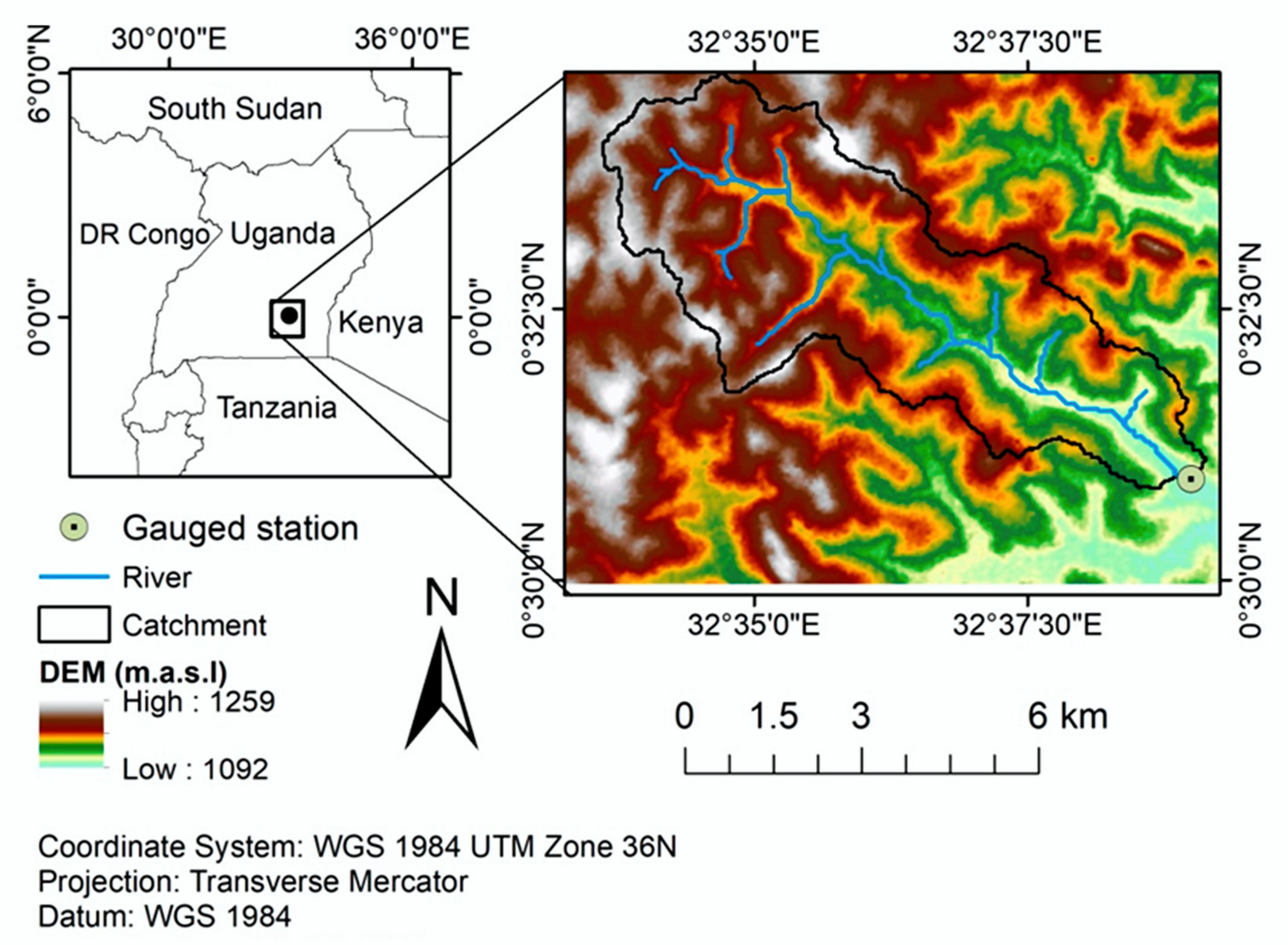
The investigated inland valley is one of the headwater micro-catchments of the Lake Kyoga basin and covers an area of 31.1 km2. The inland valley is located 30 km north of Kampala in Namulonge, Wakiso District, Central Uganda, and lies between latitude 0°30′–0°34′ N and longitude 32°34′–32°40′ E (Figure 1).
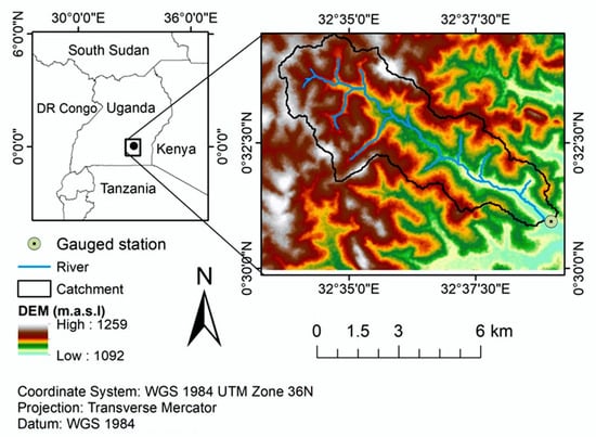
Figure 1.
Location of the study area, modified after [31].
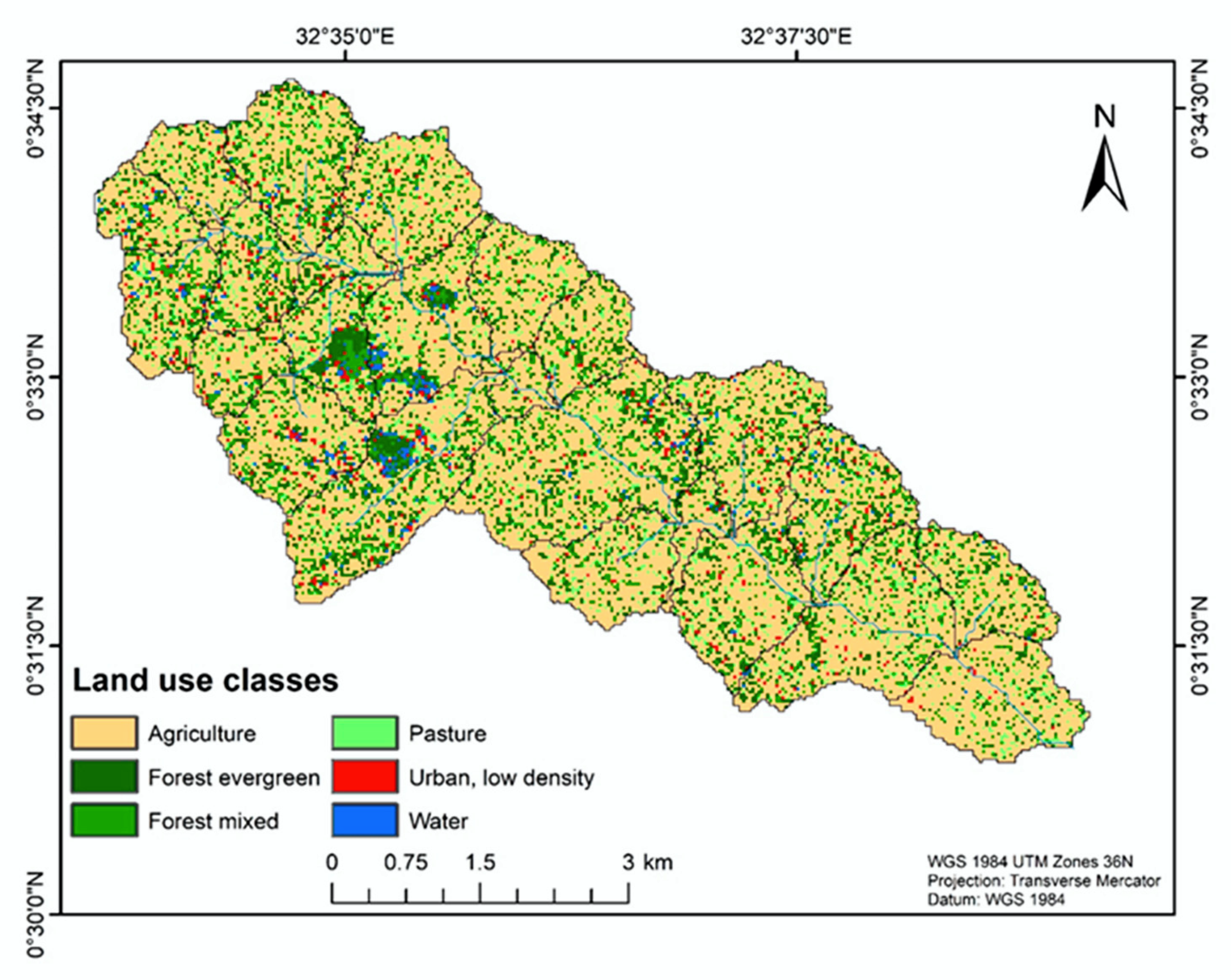
The inland valley is characterized by an undulating landscape, with gentle and wavy slopes alternating with a wetland in the valley bottom [33]. The main stream drains into Lake Kyoga through River Ssezibwa, characterized by a dense network of diverse wetlands with abundant surface and groundwater resources. The major hydrological processes in the catchment are evapotranspiration and runoff (Hortonian surface runoff and lateral flow). The runoff is due to Land use/Land cover (LULC), soil properties, and slope gradients, where steep slopes are observed along the fringes and uplands of the catchment [31]. The native vegetation in the inland valley is papyrus (Cyperus papyrus L.) and tropical rainforests, although these are significantly being converted into subsistence agriculture, with a mosaic of land uses and drainage and settlement [34]. The predominant LULC in the catchment is agriculture with an area coverage of 64.8% of the total catchment, followed by mixed forests (tropical forests) and planted eucalyptus (Figure 2) [31]. Along the valley slopes are mainly settlements and agriculture characterized by upland crops such as maize (Zea mays L.), beans (Phaseolus vulgaris L.), and sweet potatoes (Ipomoea batatas L.). The valley bottom is characterized by a mosaic of agricultural land uses such as rice (Oryza sativa L.) and taro (Colocasia esculenta L.), cultivated under saturated or near-saturated conditions. Additionally, upland crops such as maize (Zea mays L.), beans (Phaseolus vulgaris L.), sweet potatoes (Ipomoea batatas L.), and vegetables are cultivated on raised ridges in the valley bottom [34].
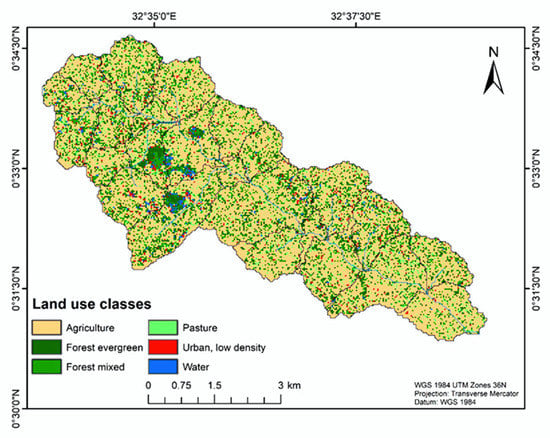
Figure 2.
Land use/Land cover (LULC) distribution in the catchment, modified after [31].
Climate in the inland valley is tropical wet and dry with a mean annual precipitation of approximately 1200 mm. Precipitation has a bimodal distribution with two rainy seasons, i.e., the first rainy season occurring from March to May (MAM, long rains) and the second rainy season from September to November (SON, short rains). The mean annual temperature is 22 °C [35]. The major soil types include rhodic Nitisols on the upper hills of the catchment, umbric Gleysols, gleyic Fluvisols, and Histosols in the valley bottom.
2.2. Hydrological Model
The Soil and Water Assessment Tool (SWAT) was used in this study to simulate the impacts of climate and LULC change on the inland valley water resources. SWAT is a continuous-time and semi-distributed hydrological model, operating at a daily time step to assess the impact of land management and climate on water, nutrient, and pesticide transport [36,37]. The model divides the catchment into sub-catchments generated from the drainage patterns derived from topographical data based on a threshold defined by the modeler. Furthermore, the sub-catchments are discretized into hydrological response units (HRUs) comprising unique combinations of soils, LULC, and slope classes [38]. Furthermore, the model is partitioned into two phases, i.e., the land phase and the channel processes. The land phase considers all processes from the event raindrop onto land surface to the stream. The land phase processes include surface runoff, lateral flow, infiltration, groundwater recharge, evapotranspiration, and groundwater flow. These hydrological processes are simulated at the HRU level, aggregated for each sub catchment to compute the overall water balance, with integration of climate data and channel processes [36]. Detailed description of the model processes can be found in [36,39], whereas model parameters are described in [38].
2.3. Model Set Up, Calibration, and Evaluation
The model set up was conducted in the ArcSWAT 2012 (revision 664) interface for ArcGIS. A digital elevation model (DEM) of 30 m resolution from Shuttle Radar Topography Mission (SRTM) was used for watershed discretization and delineation, resulting in 27 sub-catchments. Subsequently, slope, soil, and land cover data were applied for model parameterization, resulting in 174 HRUs. Land cover data were derived from Sentinel-2 images acquired in 2016 with 10 m spatial resolution [40]. SWAT was forced with meteorological data (precipitation, minimum and maximum temperature, solar radiation, relative humidity, and wind speed) from the automatic weather station of the National Crops Resources Research Institute (NaCRRI), Namulonge, located in the catchment for a period of 2014–2015. The Soil Conservation Service (SCS) curve number method was applied to calculate surface runoff and infiltration, while the Hargreaves-Samani method was used to calculate potential evapotranspiration [36]. In this method, temperature and extraterrestrial radiation are required as inputs in the model.
Distributed models require a large set of parameters for which some of them are measurable but many are hard to obtain in a direct manner [41]. Thus, in hydrological applications, parameter calibration is conducted to estimate more suitable parametric values which represent the hydrological processes of the studied catchment. After model calibration, validation is conducted to test whether the calibration is satisfactory against measured data different from those used for the calibration. For this study, the SWAT model was calibrated (for the year 2015) and validated (for the year 2016) with daily measured discharge data using the SWAT Calibration and Uncertainty Program (SWAT-CUP, version 5.1.6.2) [37,42] at the catchment outlet. SWAT-CUP is a computer program that links the SUFI-2 (Sequential Uncertainty Fitting) to SWAT and enables model sensitivity analysis, calibration, validation, and uncertainty analysis. Before calibration, a relative sensitivity analysis was conducted by applying the optimization algorithm SUFI-2 to identify the most sensitive parameters in the model [42]. SUFI-2 is an algorithm which analyzes the strength of calibration by quantifying the degree of uncertainties on the model results. Daily discharge was calculated from daily stream water level, which was continuously measured using a YSI 6-series Sondes device, Ecotech. In addition, instantaneous discharge measurements were conducted using an acoustic digital current meter (ADC, OTT Hydromet GmbH) following recommendations from [43], to establish a rating curve, which was used to calculate the time series of discharge from the daily stream water level measurements.
In this study, four quantitative statistics were applied to evaluate the performance of the model, specifically the coefficient of determination (R2, Equation 1), the Nash-Sutcliffe efficiency (NSE, Equation (2)) [44], the Kling-Gupta efficiency (KGE, Equation (3)), and the percent bias (PBIAS, Equation (4)) [45]. The coefficient of determination was used to determine what proportion of in-situ variance can be explained by the model [46]. NSE determines the relative magnitude of residual variance compared to variance of the measured data [44]. The PBIAS was calculated to measure the average tendency of the simulated discharge to be larger or smaller than the observed discharge [41]. KGE is a dimensionless statistic that is an improvement of the widely used Nash-Sutcliffe efficiency and considers different types of model errors including error in the mean, variability, and the dynamics [41]. According to Moriasi et al. [45], the model performance was considered satisfactory if R2 > 0.50, NSE > 0.50, KGE > 0.50 and the PBIAS is within the range of −25 to 25%.
where and are the measured and simulated data, respectively, and are the mean of measured and simulated data, n is the number of observations, , , and r is the linear regression coefficient between simulated and measured data. and are the standard deviation of simulated and measured data, and and are means of simulated and measured data.
2.4. Climate Change Scenarios
The impact of climate change on the water resources of the inland valley was simulated using the calibrated and validated SWAT model [31]. The meteorological input to SWAT came from six members of the CORDEX-Africa ensemble [47]. The six members were downscaled from one grid point in which the NaCRRI weather station was located. The six members listed in Table 1 were selected to represent a wide range of future precipitation signals, with increasing, decreasing, and constant precipitation patterns. The model data comprise daily data of precipitation, temperature, relative humidity, wind speed, and solar radiation and are available at a spatial resolution of 0.44° [48]. Temperature was required to simulate potential evapotranspiration using the Hargreaves-Samani method in the SWAT model. Compared to GCMs, RCMs have a higher spatial resolution and are therefore able to represent regional- and local-scale forcings [49]. Each dataset used in this study consists of a historical period (1976–2005, used as baseline/reference) and a future period (2021–2050). Climate projections under two representative concentration pathways (RCPs), namely RCP 4.5 and RCP 8.5, were used in this study. RCP 4.5 is a medium stabilization scenario where the total radiative forcing is stabilized at 4.5 Wm−2 in 2100 (approximately 650 ppm CO2 equivalent) [50]. RCP 8.5 is a scenario with total radiative forcing rising up to 8.5 Wm−2 in 2100 (approximately 1370 ppm CO2 equivalent) [51].

Table 1.
Applied Regional Climate Models (RCMs), their driving Global Climate Models (GCMs), and their corresponding abbreviations used in this study.
In order to correct for systematic biases in the RCM simulations, bias correction of precipitation and temperature data was applied. Observations from the NaCRRI weather station, which is located in the catchment, were used as observational reference. For precipitation, a non-parametric empirical quantile mapping approach [52] was applied to daily data for each month individually. For minimum and maximum temperatures, a simpler linear regression approach was used to correct daily temperatures on a monthly basis. For each member, transfer functions were derived using observed and modeled precipitation and temperature for the historical period 1976–2005. Afterwards, the same transfer functions were used to correct the regional climate projections for the period 2021–2050.
2.5. Flood Frequency and Low Flow Analysis
To determine the impacts of climate change on flood frequency and low flows in the inland valley, hydrological extreme value analysis was conducted for the simulated discharge from bias-corrected RCM data. Discharge was simulated in the validated SWAT model with the historical (1976–2005) bias-corrected RCM data for all the six models (Table 1) and with the climate projections (2021–2050) based on the RCP4.5 and RCP8.5 scenarios. The extRemes 2.0 package [53] in the statistical software R was applied to analyze the annual maximum discharge values from the six historical model runs and the climate scenarios for flood frequencies. The generalized extreme value (GEV, Equations (5) and (6)) composed of Weibull, Frechet, and Gumbel distributions, was used in combination with the generalized maximum likelihood estimation (GMLE) method, to estimate the return levels of flood events from 2-year return levels up to 50-year return levels. Then, the return levels were used to determine the changes in discharge between the historical and RCP scenarios due to climate change. Moreover, the Q10 index was calculated to estimate the flooding trend in the inland valley in addition to the annual maximum flooding approach based on the GEV analysis [54]. The Q10 index is defined here as the daily discharge value exceeded in 10% of the daily simulations and is added to the flood frequency analysis since it is less sensitive to outliers compared to the annual maximum value applied in the GEV analysis [54]:
where is the shape parameter, is the location parameter, and is the scale parameter of probability density function with > 0 and . If 0, the function becomes a Gumbel distribution as follows:
To analyse the changes in the low flows between the six historical model runs and the RCP scenarios, the Q90 index [54] was calculated. The Q90 index indicates the daily discharge value exceeded in 90% of the daily simulations. The simulations were analysed on a decadal timescale to account for the intrinsic uncertainties of the scenario simulations and to identify possible decadal trends [32]. The Q10 and Q90 were calculated using the hydrostats package in R software [55].
2.6. Land Use/Land Cover (LULC) Management Scenarios
The impact of LULC management options on water resources of the inland valley was evaluated after validation of the SWAT model. Four hypothetical future LULC management options were developed and explored in addition to the reference/current LULC applied for calibration and validation of the model from a previous study [31]. The hypothetical LULC management options were developed due to lack of a series of detailed LULC maps at the scale of the studied catchment for the previous years which would allow LULC change analysis over time. The hypothetical LULC management options were developed based on the functional landscape approach (FLA) [10] and the ongoing LULC changes and management efforts in the inland valleys of Uganda and in East Africa. FLA recognizes a wetland-catchment linkage as a fulcrum for sustainable wetland use and water resources management. The four LULC management options include: 1. exploitation (LUI): which involves total conversion of the wetland valley bottom into agriculture/cropland, the wetland fringes into planted forest (such as eucalyptus trees) and the catchment slopes into agriculture and residential areas. This option represents the ongoing LULC changes and management trends within the catchment and other inland valleys in the East African region. 2. Protection of the headwater catchment (LU2): involves total protection of the headwater catchment with tropical forest, while at the lower catchment, the valley bottom is characterized by agricultural land/cropland; wetland fringes are converted into forested wetlands, while the catchment slopes are characterized by tropical rainforest. This option is adopted from the Rwanda Environmental Management Authority wetland-catchment conservation approach [31]. 3. Total Conservation (LU3): this includes total conversion of the inland valley catchment into its natural state. The valley bottom is characterized by non-forested land cover (natural papyrus), a typical vegetation of a tropical wetland in the region [56]; wetland fringes are converted into forested wetland and catchment slopes into tropical rainforests. 4. Slope conservation (LU4): includes the conversion of the valley bottom and lower slopes into cropland, wetland fringes into wetland forest, and the upper catchment slopes into tropical rainforest.
2.7. Combined Scenarios Analysis
The combined impact of climate change and land use management on the inland valley water resources was simulated using the calibrated and validated SWAT model. Eight scenario combinations were simulated in this study. Table 2 illustrates the scenario combinations used in this study.

Table 2.
Scenario combinations of climate change and different land use/land cover (LULC) management scenarios. LU1, exploitation; LU2, protection of headwater catchment; LU3, total conservation approach; and LU4, slope conservation LULC management.
3. Results
3.1. Model Performance
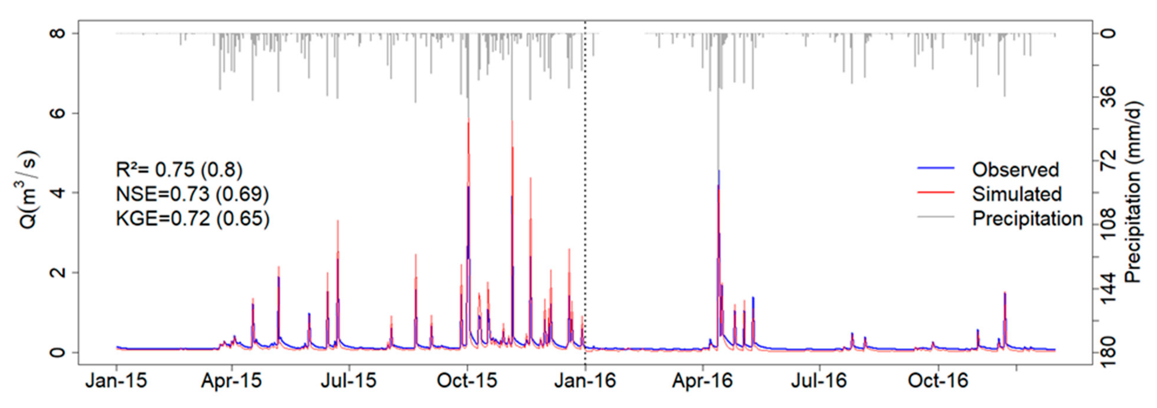
The comparison between daily observed and simulated discharge for the calibration and validation periods indicated the ability of the SWAT model to capture the flows in the inland valley, as evidenced by the model performance statistical measures (R2, NSE and KGE) (Figure 3). Notably, the model overestimated some peaks compared to the observations. Detailed model performance is explicitly shown in [31].
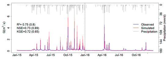
Figure 3.
Daily observed and simulated discharge for the calibration (2015) and validation (2016) periods at the catchment outlet. Statistical measures are shown in the graph. R2 is the coefficient of determination, KGE is the Kling-Gupta efficiency and NSE is the Nash-Sutcliffe efficiency. The parentheses values are for the validation period (Figure modified after [31]).
3.2. Projected Climate Changes
3.2.1. Bias Correction
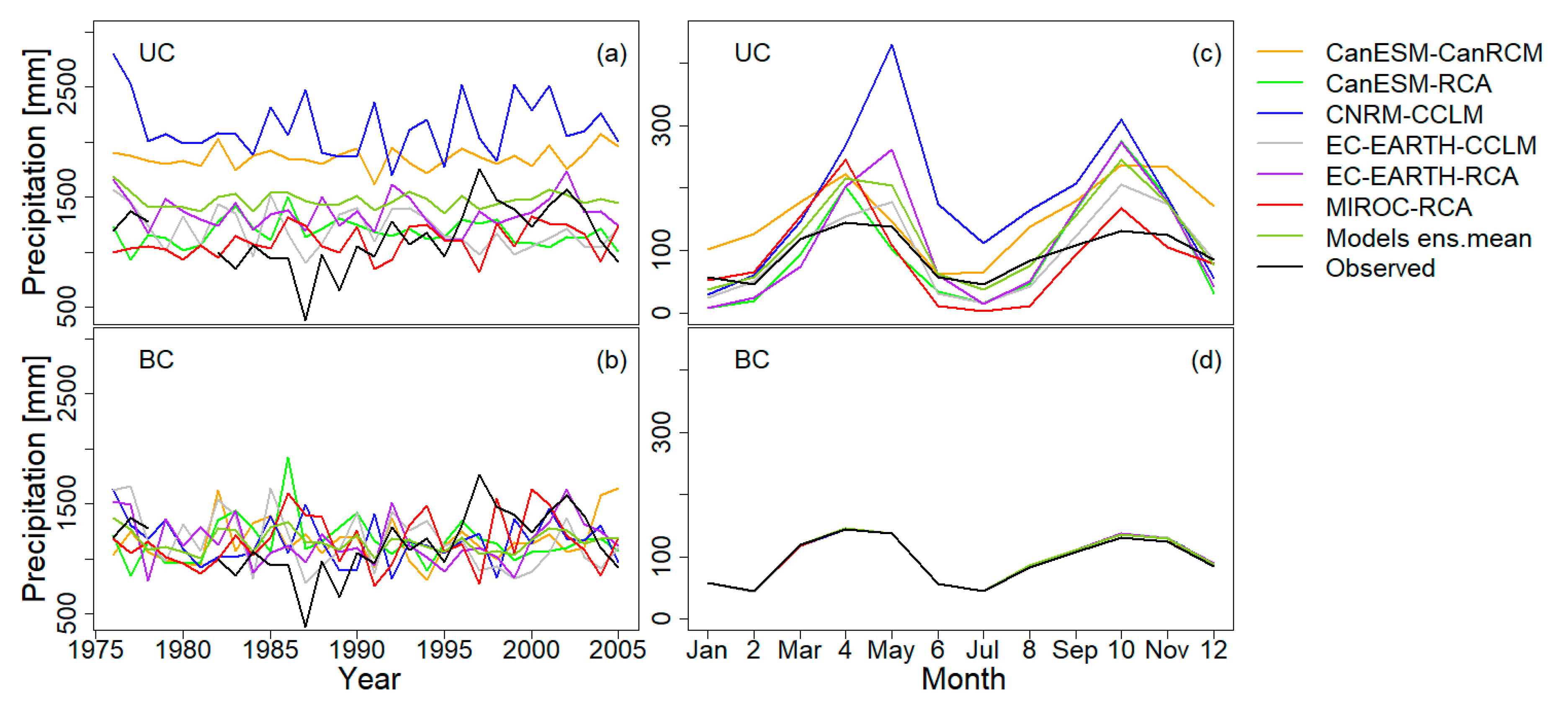
Figure 4 illustrates the annual and mean monthly time series of the observed and historical precipitation for all the six models within the period 1976–2005, with and without bias correction. The deviation among the non-bias-corrected (UC) data (Figure 4a,c) is clear. However, a significant improvement in the annual precipitation is achieved after bias correction (BC, Figure 4b). Moreover, a better agreement with virtually no deviations for the mean monthly precipitation is noted (Figure 4d). The monthly difference in precipitation among the six RCMs and the observations before bias correction ranges from −50 to +292 mm and from −1 to +6 mm after bias correction.
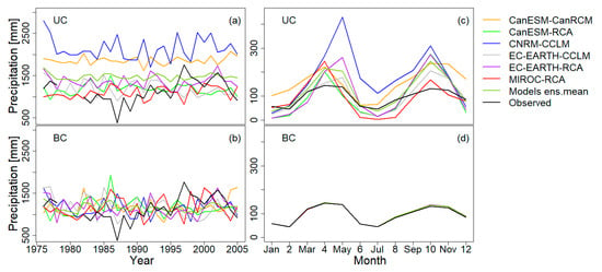
Figure 4.
Historical annual (a,b) and mean monthly (c,d) precipitation (1976–2005). UC is non-bias-corrected data and BC is bias-corrected data.
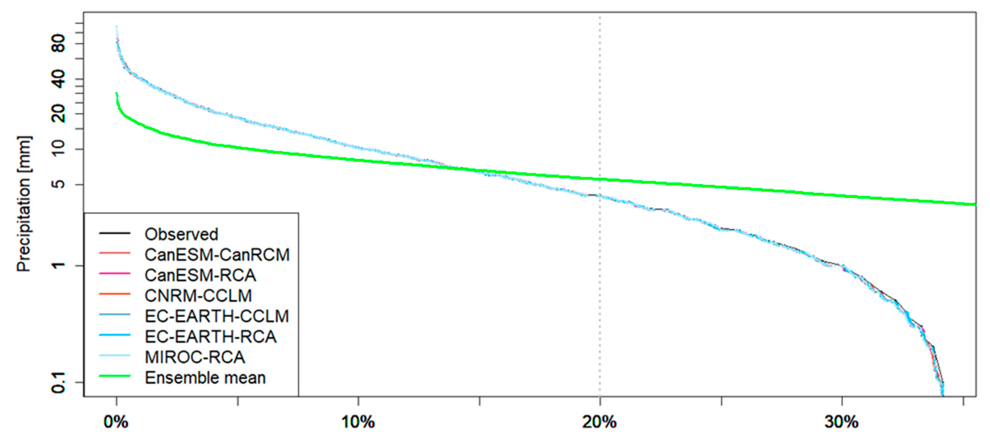
Figure 5 shows the exceedance probability for the observed and bias-corrected precipitation for the RCMs in the inland valley. All the individual RCMs exhibit a good performance of the cumulative distribution of precipitation events. Not surprisingly, the ensemble mean of the six climate models presents a different distribution of the ranked precipitation events. The ensemble mean reveals that a high number of precipitation events below 10 mm occur when compared to observations and the individual model results.

Figure 5.
Exceedance probability for the six bias-corrected RCMs, their ensemble mean (arithmetic mean), and the daily observed precipitation for the period 1976–2005. Missing precipitation values were ignored in this illustration. Dry days were included in computation of the probability curve. Exceedance probability lines for observed precipitation and models are superimposed due to their similar exceedance probabilities after bias correction.
The simulated mean monthly temperature for the period 1976–2005 shows a significant deviation from the observations, with underestimations of mean temperature using the individual models before bias correction (Figure 6). However, there is an improvement in the representation of the mean monthly temperature using the models with regard to the ground observations after bias correction, although there are some differences between the RCMs and the observation data (Figure 6).

Figure 6.
Mean monthly temperatures (1976–2005). UC is non-bias-corrected, BC is bias-corrected.
3.2.2. Projected Climate Changes
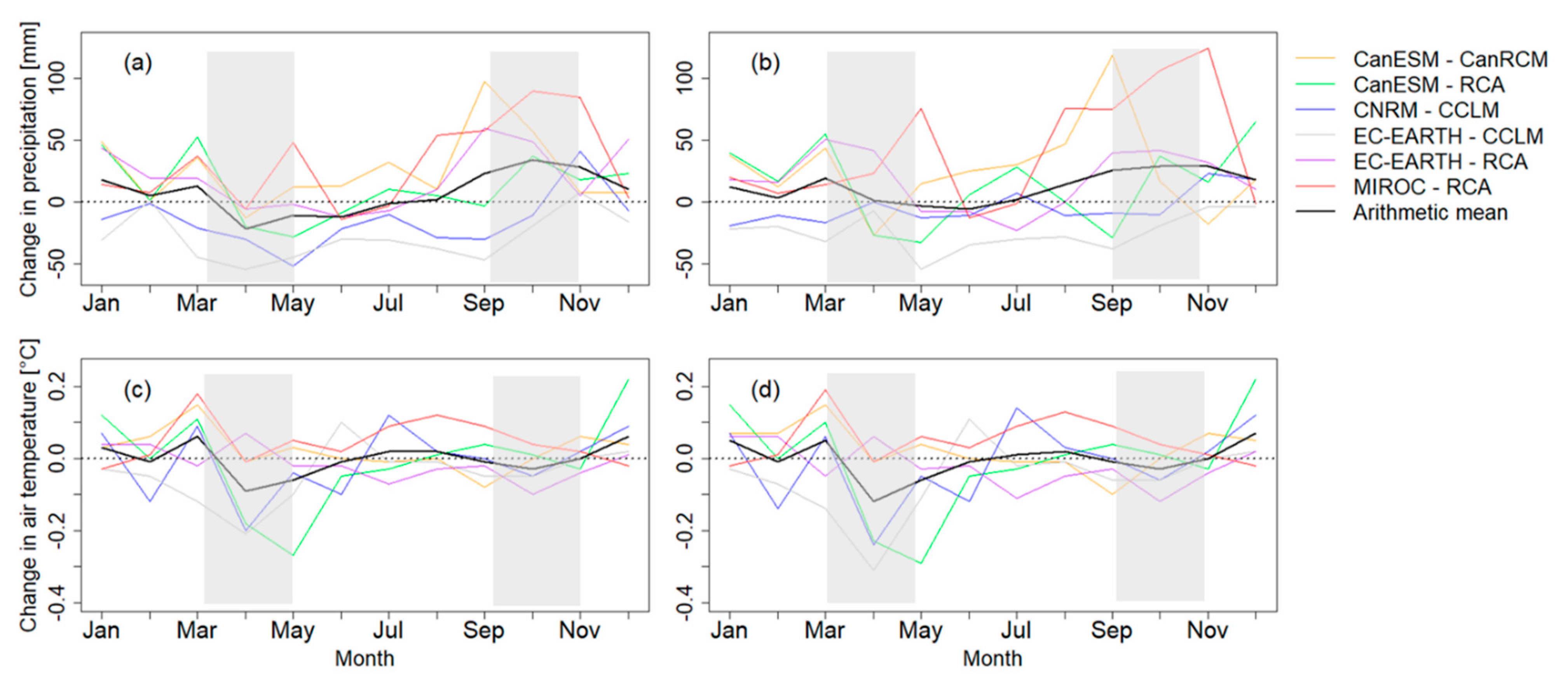
Figure 7 displays the projected monthly changes in precipitation and air temperature for all the six RCMs by comparing the bias-corrected historical model runs with the bias-corrected projections under the RCP scenarios. The RCMs exhibit uncertain changes in mean precipitation for the future (2021–2050) period for both RCP scenarios (Figure 7a,b). The ensemble mean indicates a decrease in precipitation during the long rains (MAM) and an increase in the short rains (SON) and the dry season (JJA) for RCP4.5 (Figure 7a). For RCP8.5 (Figure 7b), the ensemble mean shows an increase in precipitation throughout the wet seasons and a slight decrease (very close to 0 mm) during the dry season (JJA). Individual climate models project a much more complex intra-annual precipitation change. All models show an increase in precipitation during the dry season (JJA) except for CNRM-CCLM and EC-EARTH-CCLM under RCP4.5 and EC-EARTH-RCA and EC-EARTH-CCLM under RCP8.5. In the wet seasons, individual models project an increase in precipitation except for EC-EARTH-CCLM and CNRM-CCLM for both climate scenarios. The highest increase occurs in November with 125 mm (MIROC-RCA, RCP8.5), whereas the highest decrease is projected in April (RCP4.5) and May (RCP8.5) with −55 mm for both months (EC-EARTH-CCLM). In general, wetter conditions are projected to occur during the short rains (SON) than the long rains (MAM) for the two climate scenarios.
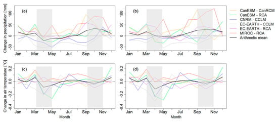
Figure 7.
Projected changes in mean monthly precipitation and air temperature for the future period 2021–2050 in comparison with 1976–2005. (a,c) indicate RCP4.5, and (b,d) represent RCP8.5. Shaded areas represent wet season, while unshaded areas represent dry season. Data used is bias- corrected.
Likewise, the temperature change signal shows both a decrease and an increase for the future period for the six RCMs and both scenarios (Figure 7c,d). The ensemble mean indicates a decrease in mean temperature during the wet season although a higher decrease is projected in the long rains than in the short rains, whose change is close to zero. All models show an increase in temperature in March except for EC-EARTH-CCLM and a decrease in April except for EC-EARTH-RCA for the two climate scenarios. The highest increase in temperature is in March with 0.2 °C (MIROC-RCA, RCP4.5 and RCP8.5), whereas the highest decrease is −0.3 °C in April (CanESM-RCA, RCP8.5) and May (CanESM-RCA, RCP4.5, and RCP8.5). MIROC-RCA shows a general increase in temperature throughout the year for the two scenarios except for the months of January, April, and December where the temperature decreases by less than 0.1 °C.
3.3. Impacts of Climate Change on Water Resources
3.3.1. Projected Changes in the Catchment Water Balance
Table 3 shows the projected changes for selected water balance components for the six RCMs under the two RCP scenarios. The ensemble mean projects a wetter future with 85.8 mm (RCP4.5) and 145 mm (RCP 8.5) additional precipitation. However, the change in annual precipitation shows high variability across individual models (ranging from −347.7 mm to +508.8 mm). The CanESM- CanRCM, CanESM-RCA, EC-EARTH-RCA, and MIROC-RCA project a wetter future for both climate scenarios, although RCP8.5 shows a higher increase in annual precipitation of up to +508.8 mm (43.9%). CNRM-CCLM and EC-EARTH-CCLM indicate a drier future for the two RCP scenarios, although there is a significant variation (−347.7 to −54.5 mm) with regard to these two RCMs and the RCP scenarios. Potential evapotranspiration, ETp, shows an increasing trend in all the RCMs from 3.7 mm to 10.6 mm. Changes in actual evapotranspiration, ET0, deep aquifer recharge, surface runoff, and water yield (summation of surface runoff, lateral flow, and groundwater flow/base flow) are closely similar to the precipitation trends, albeit their magnitude varies. The variations are more pronounced for changes in deep aquifer recharge (36.2 to 62.7 mm), surface runoff (52.2 to 72.0 mm), and water yield (59.7 to 87.8 mm) than changes in ET0 (−10.6 to −6.2 mm).

Table 3.
Projected changes in selected water balance components simulated for the period 2021–2050 based on RCP4.5 and RCP8.5 scenarios relative to the period 1976–2005. Historical annual average precipitation is based on bias-corrected RCM simulations (1976–2005). For each water balance component (except the historical precipitation) and RCP scenario, the highest and lowest values based on the absolute changes are highlighted in light blue and red, respectively. ETp represents potential evapotranspiration, ET0 is the actual evapotranspiration, SQ is surface runoff, and WYLD is the overall water yield.
3.3.2. Projected Changes in Discharge
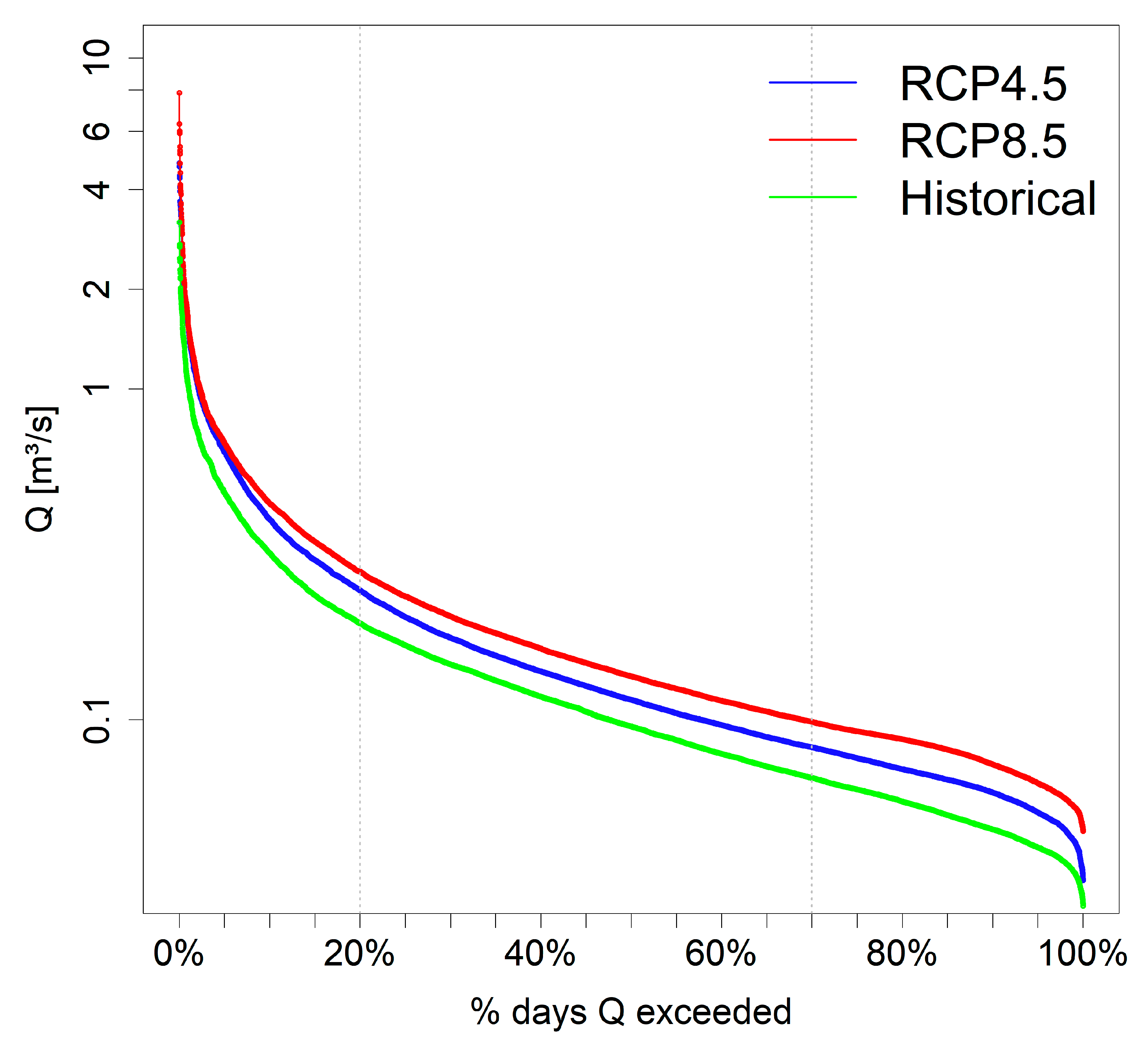
The impact of climate change on the exceedance probability of annual discharge is illustrated in the flow duration curve (FDC) (Figure 8). The RCM ensemble mean for both RCP scenarios projects a likelihood of more low and high flows compared to the historical flows due to the high projected precipitation. In this study, low flow indicates the minimum flow in the river during the dry periods of the year, while high flow is the maximum flow in the river during the wet season. Taking into account the variability of the projections, RCP8.5 projects higher total discharge in the inland valley than RCP4.5. Consequently, an increase in the discharge components such as groundwater flow, lateral flow, and surface runoff occurs, which will upsurge low and high flows during the dry and wet seasons in the inland valley, respectively.
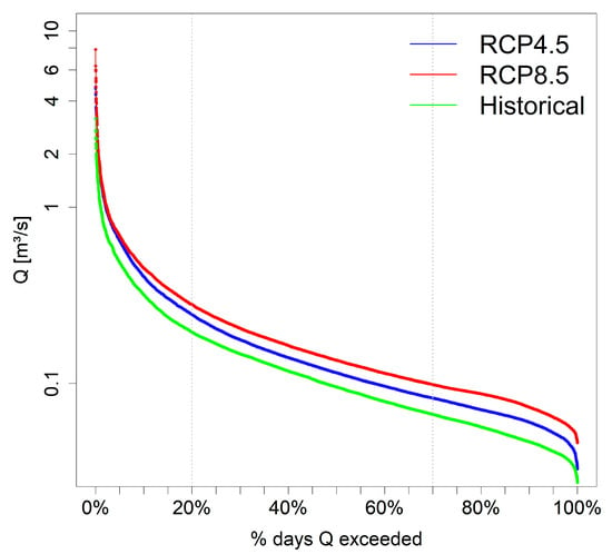
Figure 8.
Impact of climate change on the exceedance probability of daily discharge in the inland valley. The y-axis is plotted on a log scale. Daily discharge is simulated using bias-corrected daily precipitation from historical (1976–2005) and future (2021–2050) periods.
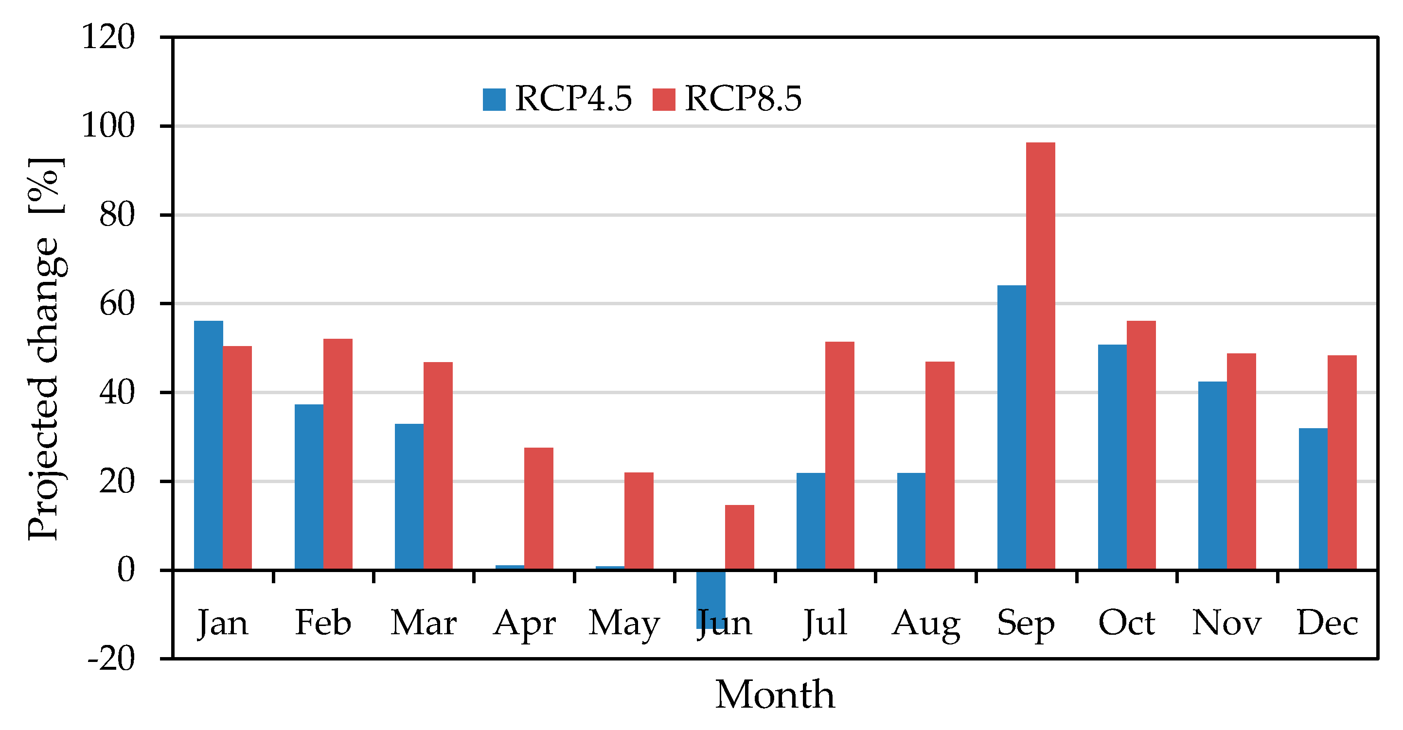
Figure 9 depicts the intra-annual variability in mean monthly discharge projected by the RCM ensemble mean for the two RCP scenarios. The mean monthly discharge will be seasonally affected by the changes in precipitation. In fact, there is a distinct difference between the wet seasons and dry (JJA and DJF) seasons. More discharge is projected in the long and short rains, although a larger magnitude is noticed in the short rains. As expected, low discharge will be more pronounced during the dry seasons and higher discharge will occur in the short rains (with an increase of 42.5% to 96%) than in the long rains (with an increase of 0.9% to 46.8%) for both RCP scenarios, although the changes are more pronounced under RCP8.5 (Figure 10).

Figure 9.
Box plots for the projected monthly average discharges under climate scenarios RCP4.5 (a) and RCP8.5 (b). Shaded area represents wet seasons (long and short rains) and unshaded area represents dry seasons.
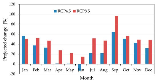
Figure 10.
Change in projected monthly discharge under climate scenarios RCP4.5 and RCP8.5.
3.3.3. Changes in Flood Frequency and Low Flows
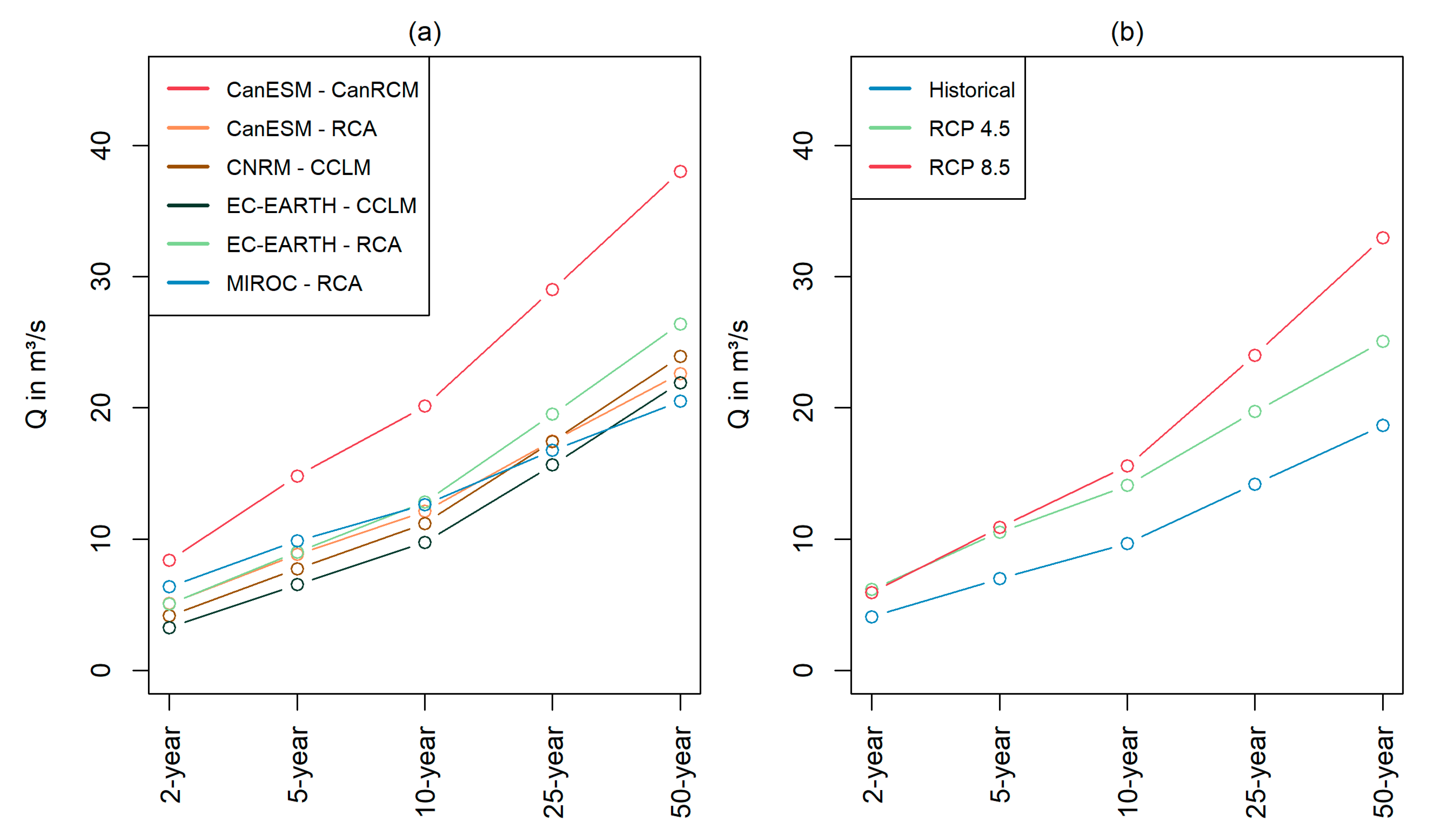
Figure 11 clearly shows the impact of climate change (Figure 11b) on the highest daily discharge over the year and the uncertainty range among the different climate models (Figure 11a). Figure 11a illustrates the return periods among the six utilized models. There is an increasing trend in discharge values with respect to the increasing return periods. However, if climate model CanESM–CanRCM is used as input data, SWAT simulates much higher discharge compared to the other five models, especially for the 25 year and 50 year return periods. RCP4.5 and RCP8.5 scenarios show an increasing intensity of flooding events compared to the historical return periods, although RCP8.5 is higher than RCP4.5 (Figure 11b). In general, the differences in the return period values between RCP4.5 and RCP8.5 are small compared to the historical return periods, except for the 50 year return period, where the difference between RCP8.5 and RCP4.5 is larger than that between RCP4.5 and historical.
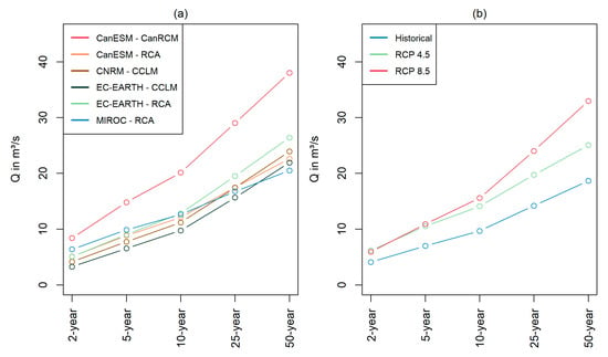
Figure 11.
Impact of climate change on the return periods of the highest daily discharge over the year. (a) is the arithmetic mean for each model across the two RCP scenarios, and (b) is the arithmetic mean for each climate scenario across all six models.
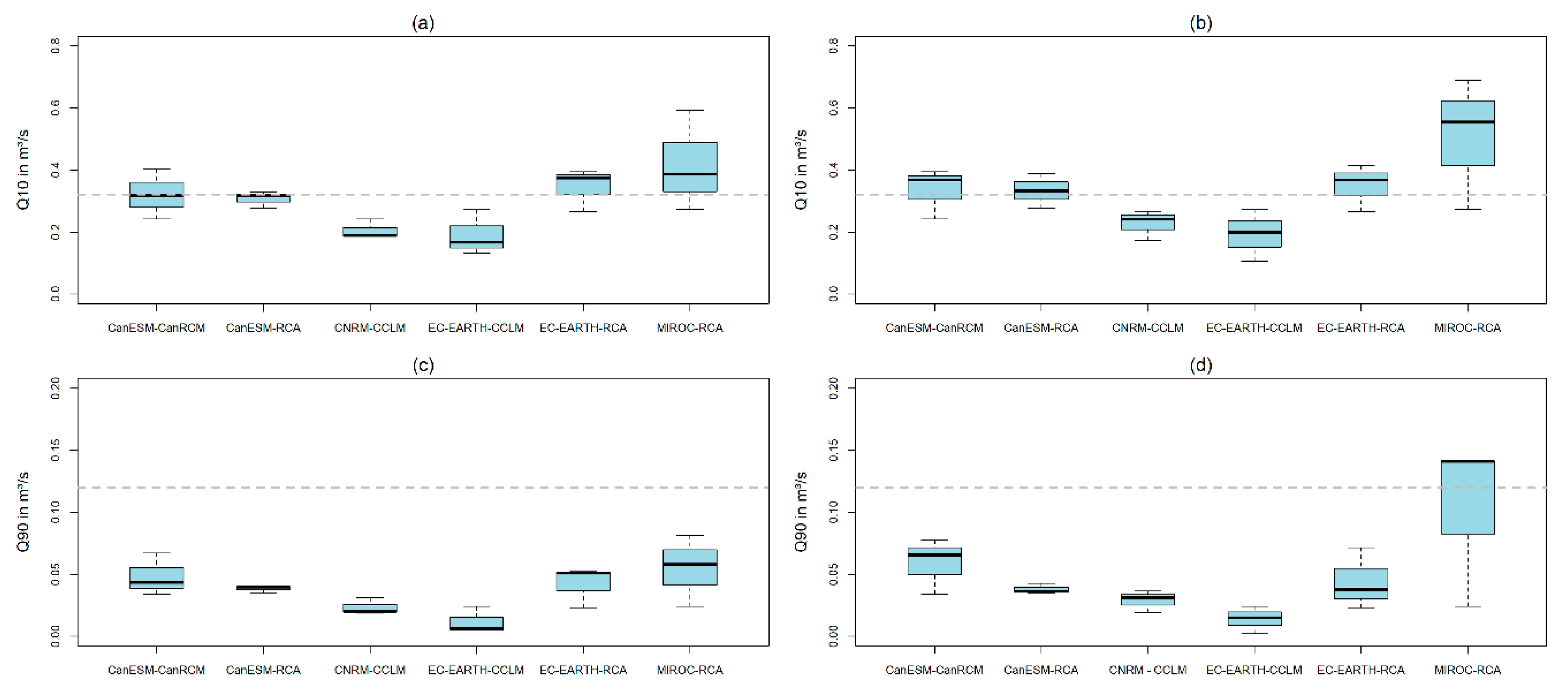
The high and low flow conditions for the historical model runs and the future climate scenarios for each model are presented in Figure 12. Historical model ensemble mean is represented by one value (dashed line) for each of the Q10 and Q90 for the entire simulation period of 1976 to 2005. Results indicate that high flow (Q10) is projected to increase for all the models across the climate scenarios except for EC-EARTH-CCLM and CNRM-CCLM with regard to the historical model runs. MIROC-RCA projects higher Q10 values compared to the other models. All the model simulated Q90 values are below the historical Q90 values for the two RCP scenarios except for the MIROC-RCA model under RCP8.5.
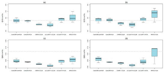
Figure 12.
Distribution of Q10 (a,b) and Q90 (c,d), representing the flow exceeded in 10% or 90% of the time for Q10 and Q90, respectively. a,c represents models runs within the RCP4.5 scenario from 2021 to 2050. b,d represent model results within the RCP8.5 scenario from 2021 to 2050. Dashed grey line in each graph represents modelled historical Q10 and Q90 for the period 1976–2005.
3.4. Impact of Land Use Management Scenarios on Catchment Water Balance
The annual water balance components according to the different LULC management scenarios are presented in Table 4. An increase in the LULC conservation levels (conservation > slope conservation > protection of the headwater catchment) results in a decrease of the total water yield (total discharge), deep aquifer recharge, and surface runoff. On the one hand, the exploitation LULC management approach will cause an increase in the total water yield and surface runoff. On the other hand, actual evapotranspiration increases for all land use scenarios. Details of the impacts of LULC management on the water resources of the inland valley catchment are discussed in [31].

Table 4.
Absolute and relative changes in selected water balance components due to future LULC management approaches. Current LULC (2015) was used as a reference. The simulations were conducted with historical (1976–2005) RCM data. Values in brackets () refer to the percent change for a particular water balance component due to LULC changes with regard to the reference LULC. All values are on an annual basis.
3.5. Combined Effects of Climate Change and Land Use Management Scenarios on the Water Balance
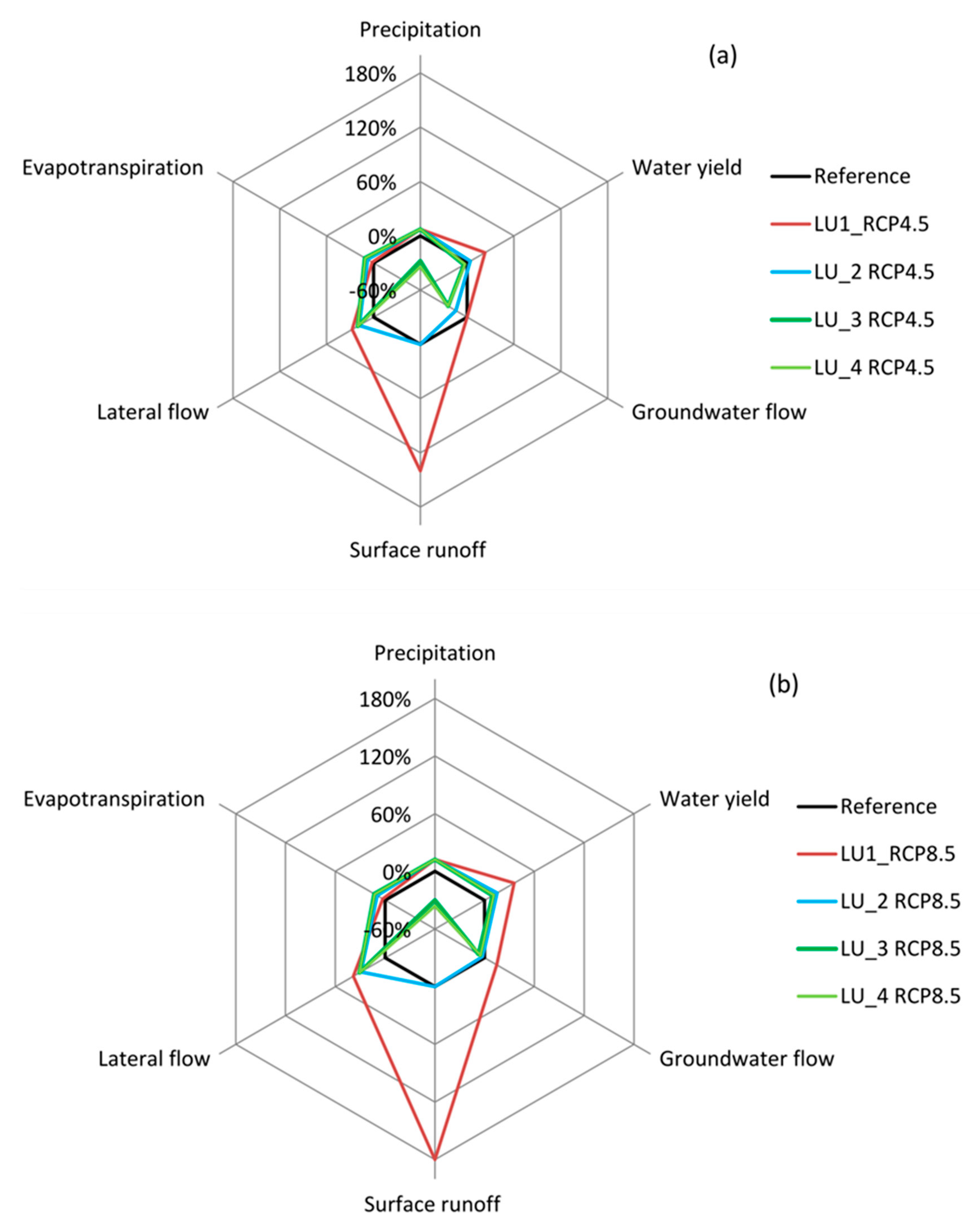
The combined impacts of climate change and LULC management scenarios on the annual water balance are shown in Table 5 and Figure 13. A marked increase in actual evapotranspiration and a decrease in surface runoff and water yield follows the order of increasing LULC management conservation levels (conservation > slope conservation > protection of headwater catchment > exploitation) and climate scenarios (RCP 8.5 > RCP 4.5). Likewise, an increase in potential evapotranspiration (0.4% to 0.7%) and in actual evapotranspiration (2% to 11%) is projected for the future (2021–2050) for the RCP scenarios (Table 5). Furthermore, annual water yield is projected to increase by 10% to 40% under RCP8.5 for all LULC scenarios. However, under RCP4.5 no uniform response of annual water yield is projected for the different LULC scenarios. For instance, exploitation and protection of headwater catchment LULC scenarios show an increase of 23% and 4% in water yield, respectively, while a decrease in the annual water yield by 4% and 3% compared to the reference/current LULC is projected under total conservation and slope conservation, respectively (Figure 13). Surface runoff and groundwater flow are projected to decrease under the total Conservation and slope conservation scenarios for both climate scenarios. A combination of each climate scenario with the protection of the headwater catchment LULC management scenario shows no effect on the surface runoff, albeit an increase in groundwater flow is projected. Continued exploitation of the inland valley in the face of climate change is projected to significantly increase surface runoff by 140% (RCP4.5, Figure 13a) and by 180% (RCP8.5, Figure 13b) in the future period.

Table 5.
Impact of combined LULC and climate change on selected water balance components. Brackets () show the relative change in the water balance components compared to the reference period with historical climate. The RCP scenario data shows the ensemble mean of all model runs.
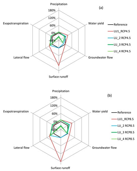
Figure 13.
Projected changes in water balance according to the combined LULC and climate scenarios. (a), represents changes under RCP4.5 and LULC; (b), represents changes under RCP8.5 and LULC; LU1, Exploitation; LU2, Protection of headwater catchment; LU3, Conservation approach; and LU4, Slope conservation LULC management. Reference includes the current land use (2015) and the historical RCM data (1976–2005).
4. Discussion
4.1. Model Performance
The calibration and validation results of the SWAT model applied to the inland valley shows the applicability of the model, which thus can be used to simulate inland valley hydrological processes. The discharge patterns for the simulations and observations during calibration and validation are captured well, with very good statistical performance according to the criteria proposed by Moriasi et al. [57]. The uncertainties in the model performance, especially an overestimation of some peaks, could be explained, for example, by measurement errors in rainfall and discharge data. Furthermore, the main stream network of the inland valley is small and shallow in depth. In combination with the ongoing poor management practices along the banks, this can cause overbank flow during severe rainfall events as observed at the gauged station in the field. However, the uncertainties are within the acceptable range for the purpose of the study of assessing the long-term effects of LULC and climate change on the water resources of the inland valley. Uncertainties in observed rainfall and discharge can only partly be wiped out by model calibration. Details of the model performance are discussed in [31].
4.2. Projected Climate Change in the Inland Valley
4.2.1. Bias Correction
The RCMs exhibit large systematic biases, which leads to high uncertainties of climate projections over the study region. [4,21,58] also report large deviations from observed precipitation and temperature exhibited by the climate models’ ensemble over East Africa. One of the reasons for the biases in projections of precipitation and temperature could be the rather low resolution of the models applied in downscaling [59,60], orographic processes, and related teleconnections, which influence precipitation variability and trends [61,62]. After bias correction, the bias in annual and monthly precipitation is significantly minimised for all the individual climate models. The varying patterns observed in annual precipitation from the models even after bias correction could be inherent model errors, which can be either random or systematic [63]. These findings are consistent with previous studies by [32,64] conducted in tropical climates. Thus, application of the chosen bias correction approaches for the study area offer representative precipitation and temperature projections, which can be used in future climate change impact studies as well as for the assessment of the potential hydrological changes for decision making and management strategies. However, as in data scarce regions, where the number of in-situ stations and data availability and quality have considerably declined and become less reliable [65], only a few in-situ observations were available for bias correction.
4.2.2. Climate Change Signal
Compared to the period of 1976–2005, a clear precipitation increase in the catchment is projected for 2021–2050 using the models ensemble mean for both RCPs. This is in line with the annual precipitation change reported by Nimusiima et al. [66] and Nimusiima et al. [67] in the Lake Kyoga basin, Uganda. They highlighted an increase in annual precipitation for both RCP scenarios for the period 2021–2050 but also noted more rainfall projected for the short rains (SON) as compared to the long rains (MAM). Furthermore, Ongoma et al. [24] found a projected increase in precipitation over East Africa for both RCP scenarios, and the authors noted larger increases in precipitation during the OND season than the MAM season.
The uncertainty in the projected changes in precipitation and temperature from the individual climate models shows a complex picture. Both wetter/drier and cool/warm conditions, respectively are expected in the future (2021–2050) period when looking at a monthly time scale for all the model combinations. This finding is also in line with [68,69] who highlight the complexity of the climate of East Africa and the necessity to adapt the former definition of the rainy seasons to the more complex reality. However, the drier periods are expected to extend to the months of April and May (well- known as rainy months [35]). Thus, a shift in the long rains in the inland valley and the Lake Kyoga basin is likely. Additionally, a warmer climate might exist during the rainy month of March. Larger increases in precipitation will occur during the short rains than long rains. It is noteworthy that within the long rains, March has the highest increase in projected precipitation, which is suitable for crop cultivation since the month coincides with the onset of the planting season in the study area and in other parts of Uganda. Nevertheless, the highest increase in precipitation throughout the whole year occurs in October/November during the short rains. Ayugi et al. [63] report similar results over East Africa, where mean seasonal precipitation is overestimated in October/November and underestimated in the long rains (MAM). Furthermore, Nsubuga and Hannes [70] report a projected increase in precipitation over Uganda during the short rains (SON), extending to DJF, while the influence on the long rains was weaker.
The projected uncertainty in the changes in precipitation and temperature are consistent with previous studies in the Lake Kyoga basin [4,71,72] and in East Africa [2,28,63,73]. Although this is only a small-scale study, it fits well to the findings of other studies from East Africa [23,73] that show a marked difference in seasonal precipitation for RCP8.5 compared to RCP4.5. Changes in temperature are less pronounced, which could also be attributed to the high amount of water in the system and the corresponding cooling effects. The variability in the projected climate change is likely to affect the stream flow regimes. During the wet seasons, there is a likelihood of higher flows resulting into flood occurrence, while in the dry season, water scarcity especially in the uplands due to the prolonged drought is likely to occur, thus increasing the pressure on the inland valleys for agricultural production.
4.3. Impact of Climate Change on Water Resources
4.3.1. Projected Changes in the Annual Water Balance
The projected increase in the selected water balance components (total water yield, surface runoff, deep aquifer recharge) as simulated by the models ensemble mean for both RCP scenarios comes with benefits and challenges in the inland valley. The benefits include increased water availability in the inland valley, and the negative implications include flood risks, which hamper the ecosystem services and functioning of the inland valley and downstream riparians. The increase in total water yield, surface runoff, and deep aquifer recharge averaged for all the six models causes a decrease in the actual evapotranspiration for both RCP scenarios, although it is more pronounced in RCP4.5, due to limited soil water availability because of less projected precipitation. Therefore, in this study, changes in mean annual precipitation may have larger impacts on the water availability of the inland valley catchment.
The high variability in the selected water balance components (total water yield, surface runoff, deep aquifer recharge, and actual evapotranspiration) simulated by the individual RCMs for the period 2021–2050 are in line with several other studies that focus on East Africa [32,55,60], although all studies were conducted at the mesoscale and macroscale. The high variability in hydrological change signal is a result of high uncertainties associated with the precipitation change projected by climate models for the catchment [74]. An increase (or decrease) in mean annual precipitation results in a larger increase (or decrease) in total water yield, surface runoff, deep aquifer recharge, and actual evapotranspiration. The projected decrease in the aforementioned water balance components from CNRM–CCLM and EC-EARTH–CCLM because of decreased precipitation may trigger long-term prevalence of water scarcity within the inland valley and may consequently lead to limited water availability downstream.
Potential evapotranspiration is increasing in all projections, whereas actual evapotranspiration is more variable, indicating a spatio-temporal water deficit within the climate models. An increase in potential evapotranspiration is not necessarily translated into an increase in actual evapotranspiration, as limitation in precipitation dictates water fluxes [75] (e.g., MIROC–RCA and CNRM–CCLM, RCP8.5, Table 3). Thus, in this study, changes in annual actual evapotranspiration are likely attributed to changes in annual precipitation, where the variations of actual evapotranspiration follow the variations of precipitation. All climate models that project a precipitation increase (CanESM–CanRCM, CanESM–RCA, EC-EARTH–RCA, MIROC–RCA) result in an increase of actual evapotranspiration due to the nearly unlimited soil water availability in the system. These finding are in line with [76] who report that changes in evapotranspiration are determined by the balance between precipitation and evaporative demand. The projected increase in monthly discharge during the rainy seasons (MAM and SON) is consistent with previous studies by [71] in the Mpologoma catchment in the Lake Kyoga basin, Eastern Uganda, and [77] in the Lake Victoria basin. On the one hand, the projected high water availability in the inland valley during the rainy seasons can bring benefits for crop production and other ecosystem services and functions. On the other hand, it may result in an increasing flood risk, more so if precipitation occurs in strong and short episodes resulting in more high flows. The higher discharge projected in the short rains than in the long rains reflects the influence of projected precipitation on discharge in the studied inland valley catchment. Therefore, any change in precipitation will have a strong impact on the discharge of the catchment; the impact will be more pronounced under RCP8.5 than RCP4.5. Nonetheless, attention should be paid to the future due to the low discharge projected in the dry seasons (JJA and DJF), which may cause water shortages for agricultural production, problems in water quality, and negative impacts on the aquatic biodiversity, as reported by [78].
4.3.2. Flood Frequency and Low Flow Analysis
The high return levels of CanESM–CanRCM relate to several reasons. One reason could be the fact that only one climate station was utilized for this small catchment, and therefore, outliers in rainfall at this station affect the whole catchment and were treated as rainfall input for the entire catchment. This is additionally aggravated by the small size of the catchment and the small response time to high rainfall amounts, which results in high discharge peaks. Furthermore, the application of the GEV with GMLE method utilized annual maximum values, although the method is susceptible to outliers and might result in high return periods. Due to this susceptibility to outliers, another method was additionally applied by using Q10 (see Figure 12a, RCP4.5 and Figure 12b, RCP8.5). As a result, CanESM-CanRCM and MIROC-RCA have higher return periods, although MIROC-RCA is wetter than CanESM-CanRCM, implying that CanESM-CanRCM has single extreme peaks and flash floods whereas MIROC-RCA has higher values for the 10% index. These results concur with a study conducted in a mesoscale floodplain catchment in Southern Tanzania [32], which showed high return periods from CanESM-CanRCM, EC-EARTH-CCLM, and MIROC-RCA, although EC-EARTH-CCLM had less pronounced effects in this study.
Flooding intensity is likely to increase with regard to the return periods in the RCP scenarios (Figure 11b). Remarkably, the impact of a more conservative scenario like RCP4.5 heavily affects the return levels of this small inland valley catchment. This might be further aggravated by LULC changes [31] leading to heavy flash floods from these inland valleys. This is of high importance for the riparians within the inland valleys, but simultaneous flash floods from the numerous inland valleys might also affect downstream riparians of the Lake Kyoga basin.
The temporal distribution of the RCM simulation results indicates a more likely wetter and drier future in the inland valley with regard to Q10 and Q90 values, respectively. This information on the performance of the climate scenarios is vital for inland valley management, especially for determining the extent of flooding in the catchment under changing land use. Thus, simulation of the impact of flash floods by utilizing a hydraulic model would provide a detailed prediction of the extent and depth of flash floods in these inland valleys and even the whole Kyoga basin under a changing climate.
4.3.3. Combined Effects of Climate and LULC Change Scenarios
LULC and climate change individually will cause changes in the selected water balance components, but more pronounced changes are expected if the drivers are combined, in particular for changes in annual water yield/discharge, surface runoff, and deep aquifer recharge. Compared to the climate change scenarios, LULC change will have a significant influence on the hydrological processes of the inland valley. The changes in patterns of the hydrological processes induced by the combined effect of climate and LULC management scenarios are consistent with the individual effect of LULC management and climate change scenarios. For example, increase in actual evapotranspiration is driven by the combined effect of projected annual precipitation change and the LULC management conservation levels (conservation > slope conservation > protection of the headwater catchment > exploitation). The observed small change in the water balance components under the exploitation LULC scenario compared to the reference/current scenario is because the catchment is close to an exploited state. The catchment is losing its natural state to agriculture, which accounts for 65% of the total catchment area [31].
Increasing LULC management conservation levels, i.e., conservation > slope conservation > protection of the headwater catchment > exploitation with the counteracting effect of climate change reduce total water yield, surface runoff, and deep aquifer recharge and increase evapotranspiration due to the increased vegetation coverage. The higher leaf area index, deep root depth, lower albedo, and higher surface roughness, transfer of energy, and momentum associated with increased vegetation cover all contribute to the increased evapotranspiration and soil infiltration and, thus, a reduction in surface runoff and total water yield in the catchment [76,77,78,79,80]. Therefore, adoption of management strategies that enhance water availability in the system will reduce the negative impacts of climate change on the water resources of the inland valleys, undergoing a paradigm shift from their pristine state to cultivation and settlement sites.
5. Conclusions
In this study, the potential implications of climate and land use management change for water balance and total discharge in a tropical inland valley in Namulonge, Central Uganda, were simulated using the SWAT model. An ensemble of six bias-corrected RCMs from the CORDEX-Africa project were utilized in the SWAT model as input to simulate the hydrological response to climate change by the mid-21st century. From the results, the following conclusions can be drawn:
- Bias correction of individual climate models improved estimates of local precipitation and temperature in relation to the ground observations in the inland valley. The applied bias correction method did not alter the annual cycle of precipitation, but its magnitude with regard to the observed precipitation.
- In the future (2021–2050), annual precipitation is projected to increase by 7.4% under RCP4.5 and by 12.5% under RCP8.5 in the inland valley. The increase in annual precipitation as projected by the ensemble mean will trigger an increase in selected catchment-averaged water balance components such as annual water yield, surface runoff, and deep aquifer recharge, as the water balance components are strongly determined by precipitation.
- Wetter conditions are expected in the short rains (SON) than in the long rains (MAM) for the two RCP scenarios. However, individual climate models project a much more complex intra-annual precipitation and temperature change, which creates considerable uncertainty about how the catchment total water yield/discharge will behave by 2050. Therefore, potential increase and decrease in future total water yield/discharge have to be considered in climate change adaptation approaches in the catchment.
- Flooding intensity is likely to increase during the rainy seasons, while the likelihood of increasing low flows is more pronounced during the dry season. Therefore, proper management options are recommended to reduce the impacts of flooding and drought in the inland valley. A detailed understanding of the possible impact of climate change on flooding extent and depth in the inland valley and downstream using a hydraulic model should be implemented for proper wetland and catchment management planning. Thus, simulation of the impact of flash floods utilizing a hydraulic model would provide a more detailed view of the future extent and depth of flash floods in these inland valleys and even the whole of Kyoga basin under the changing climate.
- LULC management and climate change individually will cause changes in the selected water balance components. More pronounced changes are expected if the drivers are combined, although future LULC management will have a significant influence on the catchment hydrological processes. Adoption of the functional landscape approach described by [10], such as conservation, slope conservation and protection of the headwater catchment management options, will reduce the impact of climate change on the water balance components such as total water yield and surface runoff. This will increase water availability and improve other ecosystem services and functions of these inland valleys undergoing a paradigm shift from their pristine state into mainly croplands in the region.
Author Contributions
Conceptualization, G.G., B.D., and C.L.; data curation, G.G.; formal analysis, G.G., K.N., and R.v.d.L.; funding acquisition, B.D. and C.L.; methodology, G.G., B.D., K.N., R.v.d.L., J.-G.M.M., and J.A.O.; software, G.G. and K.N.; supervision, B.D. and C.L.; validation, B.D. and K.N.; writing—original draft, G.G.; writing—review and editing, G.G., B.D., K.N., C.L., R.v.d.L., J.-G.M.M., and J.A.O. All authors have read and agreed to the published version of the manuscript.
Funding
This research was funded by the German Federal Ministry of Education and Research and the German Federal Ministry for Economic Cooperation and Development, under the auspices of GlobE: Wetlands in East Africa project, grant number FKZ: 031A250A-H.
Acknowledgments
The authors are grateful to the Meteorology department of the National Crops Research Resources Institute, Namulonge, for providing the historical meteorological observations, which were used for bias correction of the climate models. Further, the authors also extend gratitude to Natuhwera Malson and Robert Mutebi for their contribution in field hydrological data collection.
Conflicts of Interest
The authors declare no conflicts of interest. The founding sponsors had no role in the design of the study; in the collection, analyses, or interpretation of data; in the writing of the manuscript, and in the decision to publish the results.
References
- Christy, R.J.; Norris, B.W.; Mcnider, T.R. Surface Temperature Variations in East Africa and Possible Causes. J. Clim. 2008, 3342–3356. [Google Scholar] [CrossRef]
- Adhikari, U.; Nejadhashemi, A.P.; Woznicki, S.A. Climate change and eastern Africa: A review of impact on major crops. Food Energy Secur. 2015, 4, 110–132. [Google Scholar] [CrossRef]
- Mcdowell, G.; Ford, J.; Jones, J. Community-level climate change vulnerability research: Trends, progress, and future directions Community-level climate change vulnerability research: Trends, progress, and future directions. Environ. Res. Lett. 2016, 11, 033001. [Google Scholar] [CrossRef]
- Souverijns, N.; Thiery, W.; Demuzere, M.; Van Lipzig, N.P.M. Drivers of future changes in East African precipitation Drivers of future changes in East African precipitation. Environ. Res. Lett. 2016, 11, 114011. [Google Scholar] [CrossRef]
- Gebrechorkos, S.H.; Hülsmann, S.; Bernhofer, C. Regional climate projections for impact assessment studies in East Africa Regional climate projections for impact assessment studies in East Africa. Environ. Res. Lett. 2019, 14, 044031. [Google Scholar] [CrossRef]
- Hepworth, N.; Goulden, M. Climate Change in Uganda: Understanding the Implications and Appraising the Response; LTS Internation Ltd.: Edinburg, Scotland, 2008. [Google Scholar] [CrossRef]
- Waithaka, N.; Nelson, G.C.; Thomas, T.S.; Kyotalimye, M. East African Agriculture and Climate Change. A Comprehensive Analysis; International Food Policy Research Institute (IFPRI): Washington, DC, USA, 2013. [Google Scholar] [CrossRef]
- Government of Uganda. Uganda Wetlands Atlas Volume Two. United Nations Report 2016. Available online: https://www.mwe.go.ug/sites/default/files/Uganda (accessed on 25 May 2017).
- McCartney, M.; Morardet, S.; Rebelo, L.-M.; Finlayson, C.M.; Masiyandima, M. A study of wetland hydrology and ecosystem service provision: GaMampa wetland, South Africa. Hydrol. Sci. J. 2011, 56, 1452–1466. [Google Scholar] [CrossRef]
- Dixon, A.; Thawe, T.; Sampa, J. Striking a balance. Maintaining seasonal wetlands & their livelihood contributions in central Southern Africa Wetland. Dent. Today 2012, 31, 12. [Google Scholar]
- Junk, W.J.; An, S. Current state of knowledge regarding the world’ s wetlands and their future under global climate change: A synthesis. Aquat. Sci. 2013, 151–167. [Google Scholar] [CrossRef]
- Mitsch, W.J.; Bernal, B.; Hernandez, M.E.; Mitsch, W.J.; Bernal, B.; Ecosystem, M.E.H. Ecosystem services of wetlands. Int. J. Biodivers. Sci. Ecosyst. Serv. Manag. 2015, 11, 1–4. [Google Scholar] [CrossRef]
- Gardner, R.; Finlayson, C. Global Wetland Outlook: State of the World’s Wetlands and their Services to People; The Ramsar Convention Secretariat: Gland, Switzerland, 2018. [Google Scholar]
- Maitima, J.M.; Mugatha, S.M.; Reid, R.S.; Gachimbi, L.N.; Majule, A.; Lyaruu, H.; Pomery, D.; Mathai, S.; Mugisha, S. The linkages between land use change, land degradation and biodiversity across East Africa. Afr. J. Environ. Sci. Technol. 2009, 3, 310–325. [Google Scholar] [CrossRef]
- Von Der Heyden, C.J.; New, M.G. The role of a dambo in the hydrology of a catchment and the river network downstream. Hydrol. Earth Syst. Sci. 2003, 7, 339–357. [Google Scholar] [CrossRef]
- Mitsch, W.; Gosselink, J.G. Wetlands of the World; Wiley: Hoboken, NJ, USA, 2015; ISBN 978-1-119-01979-4. [Google Scholar]
- Wood, A.; McCartney, M. Wetland Management and Sustainable Livelihoods in Africa; Routledge: Abingdon, UK, 2013; ISBN 13 978-1-84971-411-2. [Google Scholar]
- Dixon, A.B.; Wood, A.P. Wetland cultivation and hydrological management in eastern Africa: Matching community and hydrological needs through sustainable wetland use. Nat. Resour. Forum 2003, 27, 117–129. [Google Scholar] [CrossRef]
- Windmeijer, P.N.; Andriesse, W. Inland Valleys in West Africa: An Agro-Ecological Characterization of Rice-Growing Environments; ILRI: Wageningen, The Netherlands, 1993; p. 160. [Google Scholar]
- Rodenburg, J.; Zwart, S.J.; Kiepe, P.; Narteh, L.T.; Dogbe, W.; Wopereis, M.C.S. Sustainable rice production in African inland valleys: Seizing regional potentials through local approaches. Agric. Syst. 2014, 123, 1–11. [Google Scholar] [CrossRef]
- Giertz, S.; Steup, G.; Schönbrodt, S. Use and constraints on the use of inland valley ecosystems in central Benin: Results from an inland valley survey. Erdkunde 2012, 66, 239–253. [Google Scholar] [CrossRef]
- Shongwe, M.E.; van Oldenborgh, G.J.; van den Hurk, B.; van Aalst, M. Projected changes in mean and extreme precipitation in Africa under global warming. Part II: East Africa. J. Clim. 2011, 24, 3718–3733. [Google Scholar] [CrossRef]
- Akurut, M.; Willems, P.; Niwagaba, C. Potential Impacts of Climate Change on Precipitation over Lake Victoria, East Africa, in the 21st Century. Water 2014, 6, 2634–2659. [Google Scholar] [CrossRef]
- Ongoma, V. Projected changes in mean rainfall and temperature over East Africa based on CMIP5 models. Int. J. Climatol. 2017, 38, 1375–1392. [Google Scholar] [CrossRef]
- Endris, H.S.; Lennard, C.; Hewitson, B.; Dosio, A.; Nikulin, G.; Artan, G.A. Future changes in rainfall associated with ENSO, IOD and changes in the mean state over Eastern Africa. Clim. Dyn. 2019, 52, 2029–2053. [Google Scholar] [CrossRef]
- Rowell, D.P.; Booth, B.B.; Nicholson, S.E.; Good, P. Reconciling past and future rainfall trends over east Africa. J. Clim. 2015, 28, 9768–9788. [Google Scholar] [CrossRef]
- Tierney, J.E.; Ummenhofer, C.C.; DeMenocal, P.B. Past and future rainfall in the horn of Africa. Sci. Adv. 2015, 1, e1500682. [Google Scholar] [CrossRef]
- Näschen, K.; Diekkrüger, B.; Leemhuis, C.; Steinbach, S.; Seregina, L.; Thonfeld, F.; van der Linden, R. Hydrological Modeling in Data-Scarce Catchments: The Kilombero Floodplain in Tanzania. Water 2018, 10, 599. [Google Scholar] [CrossRef]
- Hyandye, C.B.; Worqul, A.; Martz, L.W.; Muzuka, A.N.N. The impact of future climate and land use/cover change on water resources in the Ndembera watershed and their mitigation and adaptation strategies. Environ. Syst. Res. 2018, 7, 7. [Google Scholar] [CrossRef]
- Näschen, K.; Diekkrüger, B.; Evers, M.; Höllermann, B.; Steinbach, S.; Thonfeld, F. The Impact of Land Use/Land Cover Change (LULCC) on Water Resources in a Tropical Catchment in Tanzania under different Climate Change Scenarios. Sustainability 2019, 11, 7083. [Google Scholar] [CrossRef]
- Gabiri, G.; Leemhuis, C.; Diekkrüger, B.; Näschen, K.; Steinbach, S.; Thonfeld, F. Modelling the impact of land use management on water resources in a tropical inland valley catchment of central Uganda, East Africa. Sci. Total Environ. 2019, 653, 1052–1066. [Google Scholar] [CrossRef] [PubMed]
- Näschen, K.; Diekkrüger, B.; Leemhuis, C.; Seregina, L.S. Impact of Climate Change on Water Resources in the Kilombero Catchment in Tanzania. Water 2019, 11, 859. [Google Scholar] [CrossRef]
- Miyamoto, K.; Maruyama, A.; Haneishi, Y.; Matsumoto, S.; Tsuboi, T.; Asea, G.; Okello, S.; Takagaki, M.; Kikuchi, M. NERICA Cultivation and its Yield Determinants: The Case of Upland Rice Farmers in Namulonge, Central Uganda. J. Agric. Sci. 2012, 4, 120–135. [Google Scholar] [CrossRef]
- Gabiri, G.; Diekkrüger, B.; Leemhuis, C.; Burghof, S.; Näschen, K.; Asiimwe, I.; Bamutaze, Y. Determining hydrological regimes in an agriculturally used tropical inland valley wetland in Central Uganda using soil moisture, groundwater, and digital elevation data. Hydrol. Process. 2018, 32. [Google Scholar] [CrossRef]
- Nsubuga, F.N.W. Climatic Trends at Namulonge in Uganda: 1947–2009. Geogr. Geol. 2000, 3, 119–131. [Google Scholar] [CrossRef]
- Neitsch, S.L.; Arnold, J.G.; Kiniry, J.R.; Williams, J. Soil & Water Assessment Tool Theoretical Documentation Version 2009; Technical Report No.406; Texas Water Resources Institute: College Station, TX, USA, 2011. [Google Scholar]
- Arnold, J.G.; Moriasi, D.N.; Gassman, P.W.; Abbaspour, K.C.; White, M.J.; Srinivasan, R.; Santhi, C.; Harmel, R.D.; Van Griensven, A.; Van Liew, M.W.; et al. Swat: Model Use, Calibration, and Validation. Trans. ASABE 2012, 55, 1491–1508. [Google Scholar] [CrossRef]
- Arnold, J.G.; Kiniry, J.R.; Srinivasan, R.; Williams, J.R.; Haney, E.B.; Neitsch, S.L. Soil & Water Assessment Tool: Input/output Documentation. Version 2012; Texas Water Resources Institute: College Station, TX, USA, 2013; p. 650. [Google Scholar]
- Arnold, J.G.; Srinivasan, R.; Muttiah, R.S.; Williams, J.R. Large area hydrologic modeling and assesment Part I: Model development. JAWRA J. Am. Water Resour. Assoc. 1998, 34, 73–89. [Google Scholar] [CrossRef]
- Drusch, M.; Del Bello, U.; Carlier, S.; Colin, O.; Fernandez, V.; Gascon, F.; Hoersch, B.; Isola, C.; Laberinti, P.; Martimort, P.; et al. Sentinel-2: ESA’s Optical High-Resolution Mission for GMES Operational Services. Remote Sens. Environ. 2012, 120, 25–36. [Google Scholar] [CrossRef]
- Gupta, H.V.; Sorooshian, S.; Yapo, P.O. Toward improved calibration of hydrologic models: Multiple and non-commensurable measures of information. Water Resour. Res. 1998, 34, 751–763. [Google Scholar] [CrossRef]
- Abbaspour, K. SWAT-CUP: SWAT Calibration and Uncertainty Programs—A User Manual. Neprashtechnology 2015. [Google Scholar] [CrossRef]
- Fenton, J.D.; Keller, R.J. The Calculation of Streamflow from Measurements of Stage; Technical Report 01/6 2001. Available online: http://johndfenton.com/Papers/Calculation-of-streamflow-from-measurements-of-stage.pdf (accessed on 15 January 2015).
- Nash, J.E.; Sutcliffe, J.V. River flow forecasting through conceptual models part I—A discussion of principles. J. Hydrol. 1970, 10, 282–290. [Google Scholar] [CrossRef]
- Moriasi, D.N.; Arnold, J.G.; Van Liew, M.W.; Binger, R.L.; Harmel, R.D.; Veith, T.L. Model evaluation guidelines for systematic quantification of accuracy in watershed simulations. Trans. ASABE 2007, 50, 885–900. [Google Scholar] [CrossRef]
- Rathjens, H.; Oppelt, N. SWAT model calibration of a grid-based setup. Adv. Geosci. 2012, 32, 55–61. [Google Scholar] [CrossRef]
- Gutowski, J.W.; Giorgi, F.; Timbal, B.; Frigon, A.; Jacob, D.; Kang, H.S.; Raghavan, K.; Lee, B.; Lennard, C.; Nikulin, G.; et al. WCRP COordinated Regional Downscaling EXperiment (CORDEX): A diagnostic MIP for CMIP6. Geosci. Model Dev. 2016, 9, 4087–4095. [Google Scholar] [CrossRef]
- Nikulin, G.; Jones, C.; Giorgi, F.; Asrar, G.; Büchner, M.; Cerezo-Mota, R.; Christensen, O.B.; Déqué, M.; Fernandez, J.; Hänsler, A.; et al. Precipitation climatology in an ensemble of CORDEX-Africa regional climate simulations. J. Clim. 2012, 25, 6057–6078. [Google Scholar] [CrossRef]
- Kim, J.; Waliser, D.E.; Mattmann, C.A.; Goodale, C.E.; Hart, A.F.; Zimdars, P.A.; Crichton, D.J.; Jones, C.; Nikulin, G.; Hewitson, B.; et al. Evaluation of the CORDEX-Africa multi-RCM hindcast: Systematic model errors. Clim. Dyn. 2014, 42, 1189–1202. [Google Scholar] [CrossRef]
- Thomson, A.M.; Calvin, K.V.; Smith, S.J.; Kyle, G.P.; Volke, A.; Patel, P.; Delgado-Arias, S.; Bond-Lamberty, B.; Wise, M.A.; Clarke, L.E.; et al. RCP4.5: A pathway for stabilization of radiative forcing by 2100. Clim. Chang. 2011, 109, 77–94. [Google Scholar] [CrossRef]
- Riahi, K.; Rao, S.; Krey, V.; Cho, C.; Chirkov, V.; Fischer, G.; Kindermann, G.; Nakicenovic, N.; Rafaj, P. RCP 8.5—A scenario of comparatively high greenhouse gas emissions. Clim. Chang. 2011, 109, 33–57. [Google Scholar] [CrossRef]
- Gudmundsson, L.; Bremnes, J.B.; Haugen, J.E.; Engen-Skaugen, T. Technical Note: Downscaling RCM precipitation to the station scale using statistical transformations; A comparison of methods. Hydrol. Earth Syst. Sci. 2012, 16, 3383–3390. [Google Scholar] [CrossRef]
- Gilleland, E.; Katz, R.W. extRemes 2.0: An Extreme Value Analysis Package in R. J. Stat. Softw. 2016, 72. [Google Scholar] [CrossRef]
- Van Vliet, M.T.H.; Franssen, W.H.P.; Yearsley, J.R.; Ludwig, F.; Haddeland, I.; Lettenmaier, D.P.; Kabat, P. Global river discharge and water temperature under climate change. Glob. Environ. Chang. 2013, 23, 450–464. [Google Scholar] [CrossRef]
- Bond, N. Hydrostats: Hydrologic Indices for Daily Time Series Data; R Foundation for Statistical Computing: Vienna, Austria, 2018. [Google Scholar]
- Okeyo-Owuor, J.B.; Raburu, P.O. Wetlands of Lake Victoria basin, Kenya: Distribution, Current Status and Conservation Challenges. Community Based Approach to Management of Nyando Wetland, Lake Victoria Basin, Kenya. 2016, pp. 2–3. Available online: https://www.oceandocs.org/bitstream/handle/1834/7721/ktf0424.pdf?sequence=1 (accessed on 27 May 2018).
- Moriasi, D.N.; Gitau, M.W.; Pai, N.; Daggupati, P. Hydrologic and Water Quality Models: Performance Measures and Evaluation Criteria. Trans. ASABE 2015, 58, 1763–1785. [Google Scholar]
- Vanderkelen, I.; Van Lipzig, N.P.M.; Thiery, W. Modelling the water balance of Lake Victoria (East Africa)—Part 2: Future projections. J. Hydrol. Earth Syst. Sci. 2018, 22, 5527–5549. [Google Scholar] [CrossRef]
- Bruyère, C.L.; Done, J.M.; Holland, G.J.; Fredrick, S. Bias corrections of global models for regional climate simulations of high-impact weather. Clim. Dyn. 2013, 43, 1847–1856. [Google Scholar] [CrossRef]
- Maraun, D. Bias Correcting Climate Change Simulations—A Critical Review. Curr. Clim. Chang. Rep. 2016, 2, 211–220. [Google Scholar] [CrossRef]
- Ogwang, B.A.; Chen, H.; Li, X.; Gao, C. The Influence of Topography on East African October to December Climate: Sensitivity Experiments with RegCM4. Adv. Meteorol. 2014, 2014, 1–14. [Google Scholar] [CrossRef]
- Camberlin, P.; Okoola, R.E. The onset and cessation of the ‘long rains’ in eastern Africa and their interannual variability. Theor. Appl. Climatol. 2003, 75, 43–54. [Google Scholar] [CrossRef]
- Ayugi, B.; Tan, G.; Tchalim, G.; Ojara, M.; Ongoma, V. Historical evaluations and simulations of precipitation over East Africa from Rossby centre regional climate model. Atmos. Res. 2020, 232, 104705. [Google Scholar] [CrossRef]
- Trinh-Tuan, L.; Matsumoto, J.; Tangang, F.T.; Juneng, L.; Cruz, F.; Narisma, G. Application of Quantile Mapping Bias Correction for Mid-future Precipitation Projections over Vietnam Application of Quantile Mapping Bias Correction for Mid-Future Precipitation Projections over Vietnam. SOLA 2019, 15, 1–6. [Google Scholar] [CrossRef]
- Malhi, Y.; Wright, J. Spatial patterns and recent trends in the climate of tropical rainforest regions. Philos. Trans. R. Soc. B Biol. Sci. 2004, 359, 311–329. [Google Scholar] [CrossRef] [PubMed]
- Nimusiima, A.; Basalirwa, C.P.K.; Majaliwa, J.G.M.; Mbogga, S.M.; Mwavu, E.N.; Namaalwa, J.; Okello-Onen, J. Analysis of Future Climate Scenarios over Central Uganda Cattle Corridor. J. Earth Sci. Clim. Chang. 2014, 5, 10. [Google Scholar]
- Nimusiima, A.; Kisembe, J.; Nakyembe, N. Evaluation of past and future extreme rainfall characteristics over Eastern Uganda. J. Environ. Agric. Sci. 2019, 18, 38–49. [Google Scholar]
- Nicholson, S.E. Climate and climate variability of rainfall over eastern Africa. Rev. Geophys. 2017, 55, 590–635. [Google Scholar] [CrossRef]
- Seregina, L.S.; Fink, A.H.; Van Der Linden, R.; Elagib, N.A.; Pinto, J.G. A new and flexible rainy season definition: Validation for Greater Horn of Africa and application to rainfall trends. Int. J. Climatol. 2018, 39, 989–1012. [Google Scholar] [CrossRef]
- Nsubuga, F.W.; Rautenbach, H. Climate change and variability: A review of what is known and ought to be known for Uganda. Int. J. Clim. Chang. Strat. Manag. 2018, 10, 752–771. [Google Scholar] [CrossRef]
- Kigobe, M.; van Griensven, A. Assessing hydrological response to change in climate: Statistical downscaling and hydrological modelling within the upper Nile. In Proceedings of the Fifth Biennial Meeting on International Congress on Environmental Modelling and Software, Modelling for Environment’s Sake, Ottawa, ON, Canada, 5–8 July 2010; Swayne, D.A., Yang, W., Voinov, A.A., Rizzoli, A., Filatova, T., Eds.; International Environmental Modelling and Software Society: Ottawa, ON, Canada, 2010; pp. 2096–2105. [Google Scholar]
- Tumusiime, M.D.; Ageet, S. Assessment of Impacts of Climate Change on Hydro-meteorological Ecosystem Services and Water Stress in Lake Kyoga Catchment. Int. J. Res. Eng. 2018, 5, 345–354. [Google Scholar] [CrossRef][Green Version]
- Rowell, D.P.; Chadwick, R. Causes of the Uncertainty in Projections of Tropical Terrestrial Rainfall Change: East Africa. J. Clim. 2018, 31, 5977–5995. [Google Scholar] [CrossRef]
- IPCC. Climate change: Impacts, adaptation, and vulnerability. In Part B: Regional Aspects. Contribution of Working Group II to the Fifth Assessment Report of the Intergovernmental Panel on Climate Change; Barros, V.R., Field, C.B., Dokken, D.J., Mastrandrea, M.D., Mach, K.J., Bilir, T.E., Chatterjee, M., Ebi, K.L., Estrada, Y.O., Genova, R.C., et al., Eds.; Cambridge University Press: Cambridge, UK; New York, NY, USA, 2014; pp. 1133–1820. [Google Scholar]
- Newman, B.D.; Wilcox, B.P.; Archer, S.R.; Breshears, D.D.; Dahm, C.N.; Duffy, C.J.; McDowell, N.G.; Phillips, F.M.; Scanlon, B.R.; Vivoni, E.R. Ecohydrology of water limited environments: A scientific vision. Water Resour. Res. 2006, 42, W06302. [Google Scholar] [CrossRef]
- Marhaento, H.; Martijn, J.; Booij, M.J.; Hoekstra, A.Y. Hydrological response to future land-use change and climate change in a tropical catchment. Hydrol. Sci. J. 2018, 63, 1368–1385. [Google Scholar] [CrossRef]
- Olaka, L.A.; Ogutu, J.O.; Said, M.Y.; Oludhe, C. Projected Climatic and Hydrologic Changes to Lake Victoria Basin Rivers under Three RCP Emission Scenarios for 2015–2100 and Impacts on the Water Sector. Water 2019, 11, 1449. [Google Scholar] [CrossRef]
- Hughes, S.J.; Cabecinha, E.; Santos, J.A.; Andrade, C.; Lopes, D.; Trindade, H.; Cabral, J.A.; Santos, M.A.; Lourenço, J.; Aranha, J.; et al. A predictive modelling tool for assessing climate, land use and hydrological change on reservoir physicochemical and biological properties. Area 2012, 44, 432–442. [Google Scholar] [CrossRef]
- Beaulieu, E.; Lucas, Y.; Viville, D.; Ackerer, P.; Godde, Y. Hydrological and vegetation response to climate change in a forested mountainous catchment. Model. Earth Syst. Environ. 2016, 2, 1–15. [Google Scholar] [CrossRef]
- Nugroho, P.; Marsono, D.; Sudira, P.; Suryatmojo, H. Impact of Land-use Changes on Water Balance. Procedia Environ. Sci. 2013, 17, 256–262. [Google Scholar] [CrossRef]
© 2020 by the authors. Licensee MDPI, Basel, Switzerland. This article is an open access article distributed under the terms and conditions of the Creative Commons Attribution (CC BY) license (http://creativecommons.org/licenses/by/4.0/).

