
Formation Flying Lyapunov-Based Control Using Lorentz Forces

 , , and
Abstract
:1. Introduction
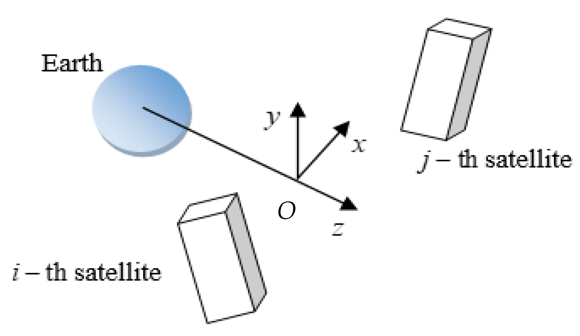
2. Problem Statement and Motion Equations
2.1. Motion Equations
2.2. Lorentz Force
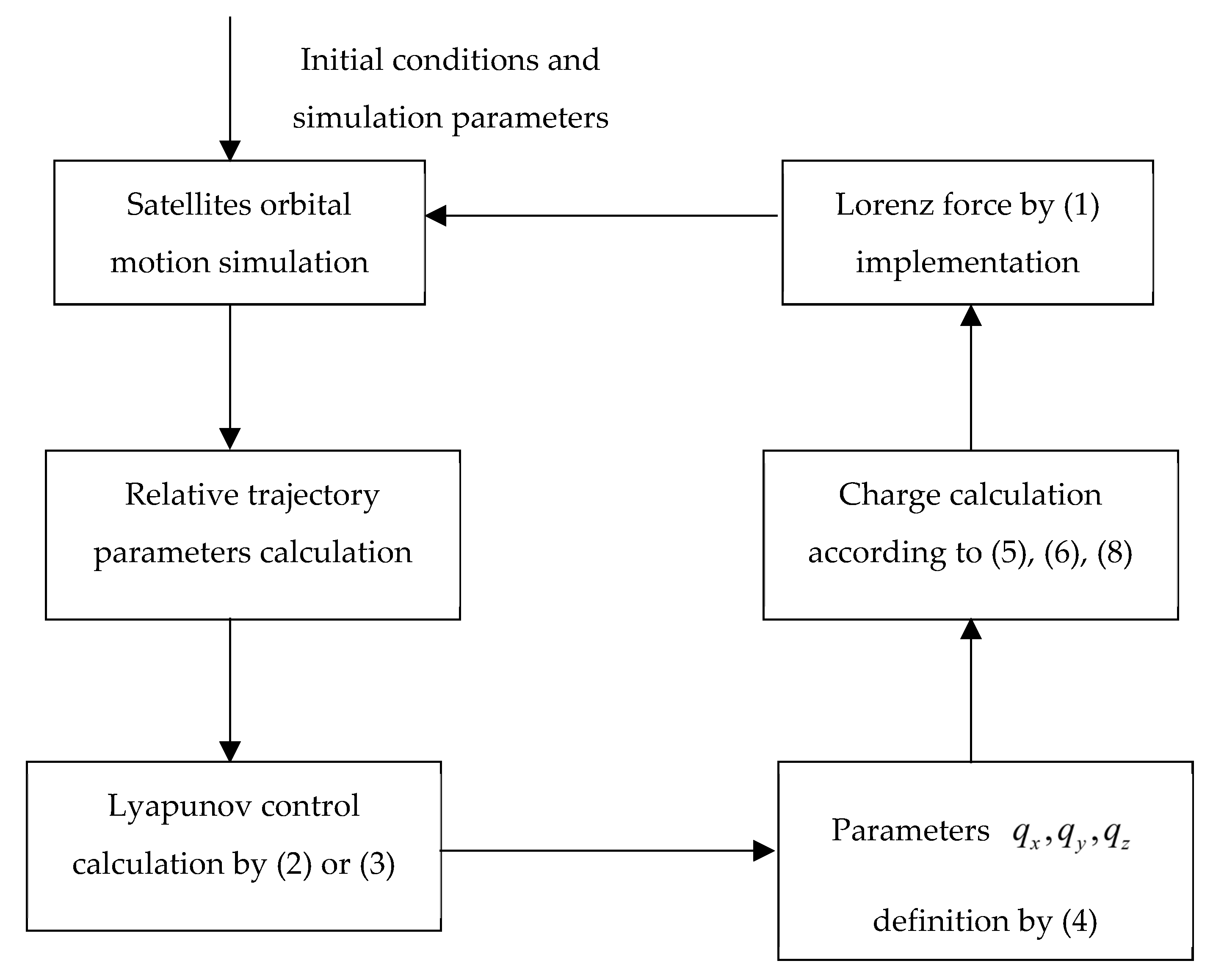
3. Control Algorithm
3.1. Lyapunov-Based Control
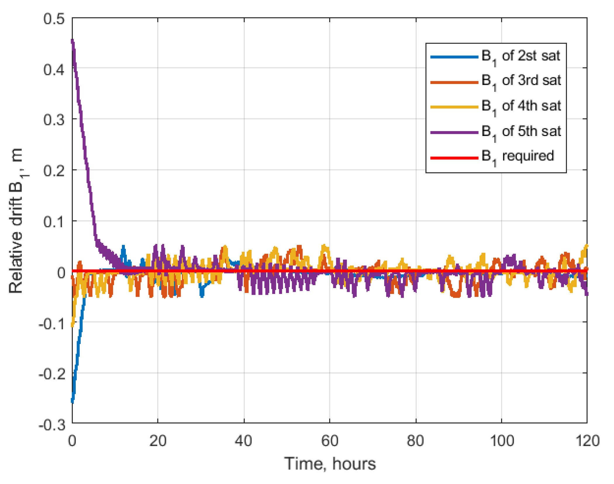
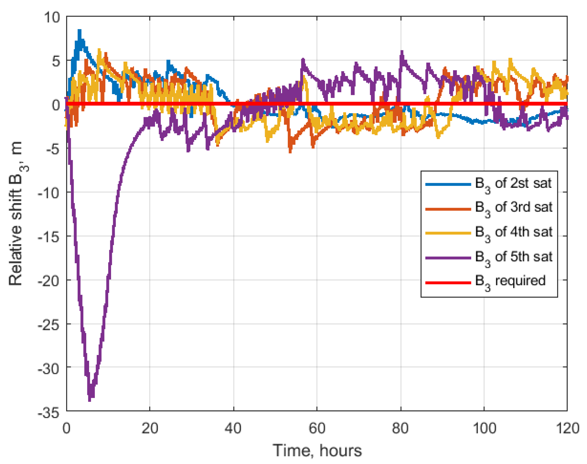
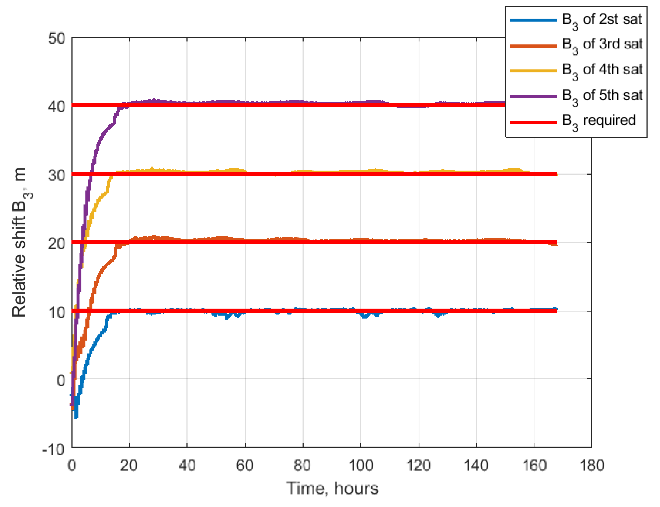
3.1.1. Relative Drift and Relative Shift Control
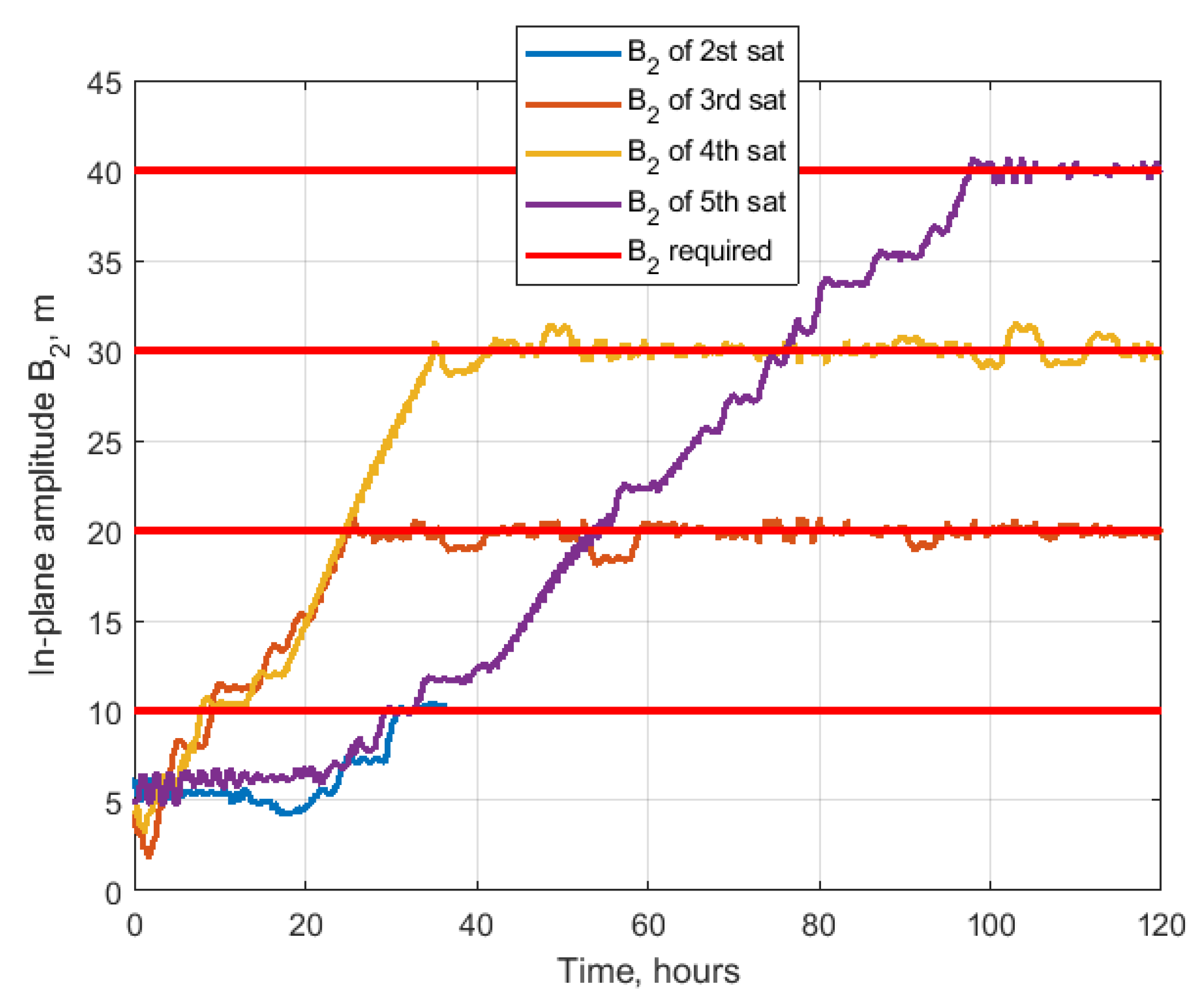
3.1.2. In-Plane and Out-of-Plane Amplitudes Control
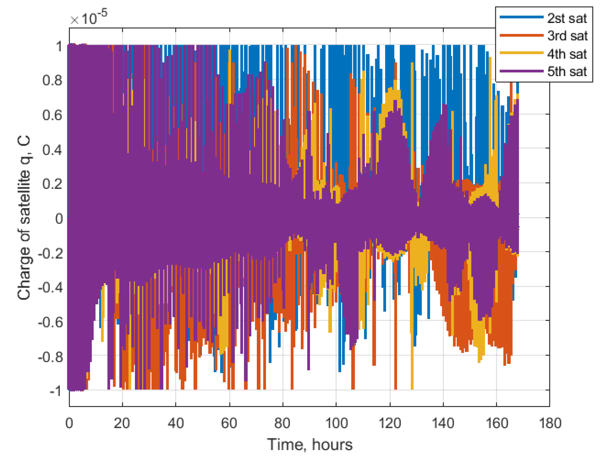
3.2. Control Implementation Using Lorenz Force
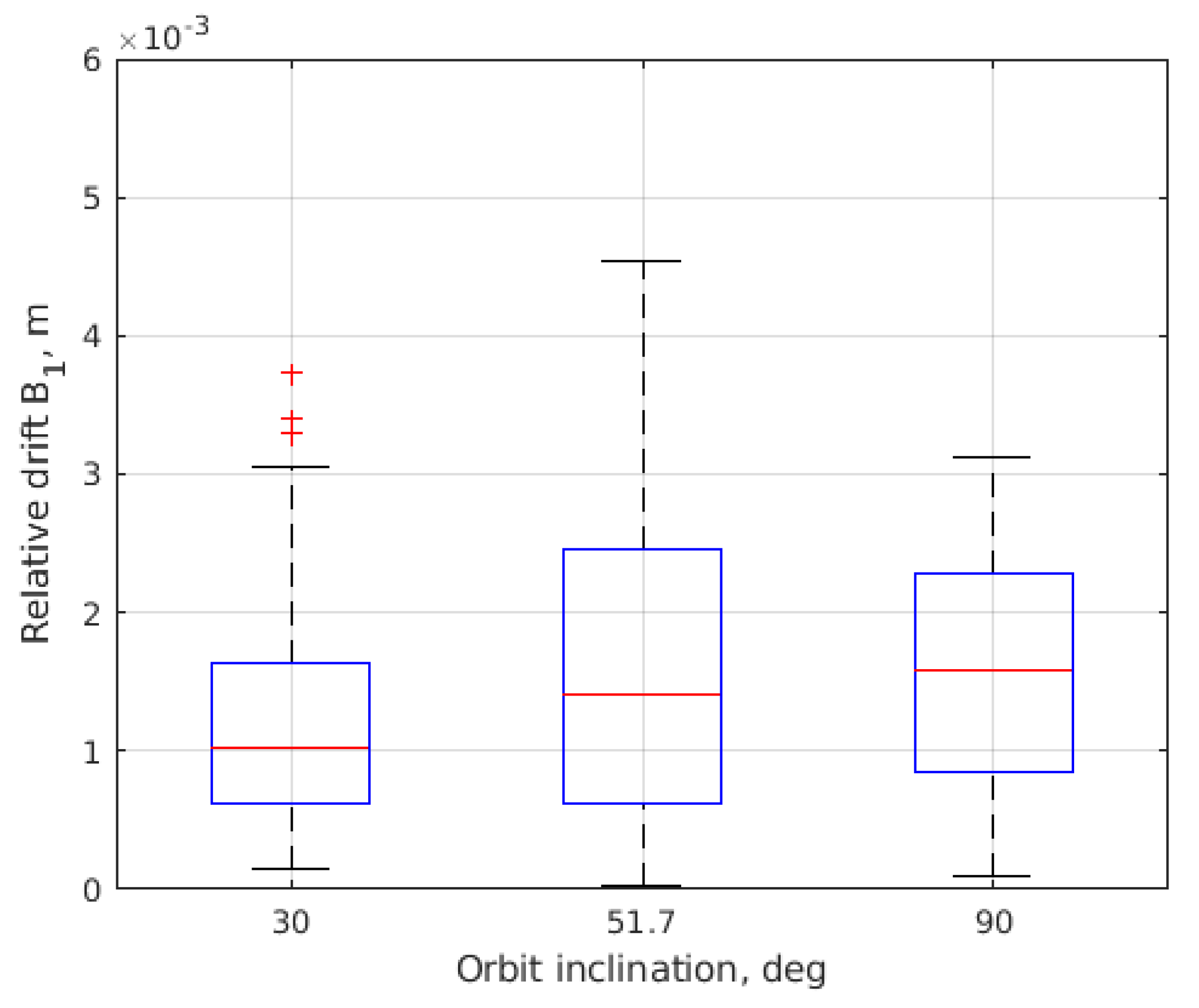
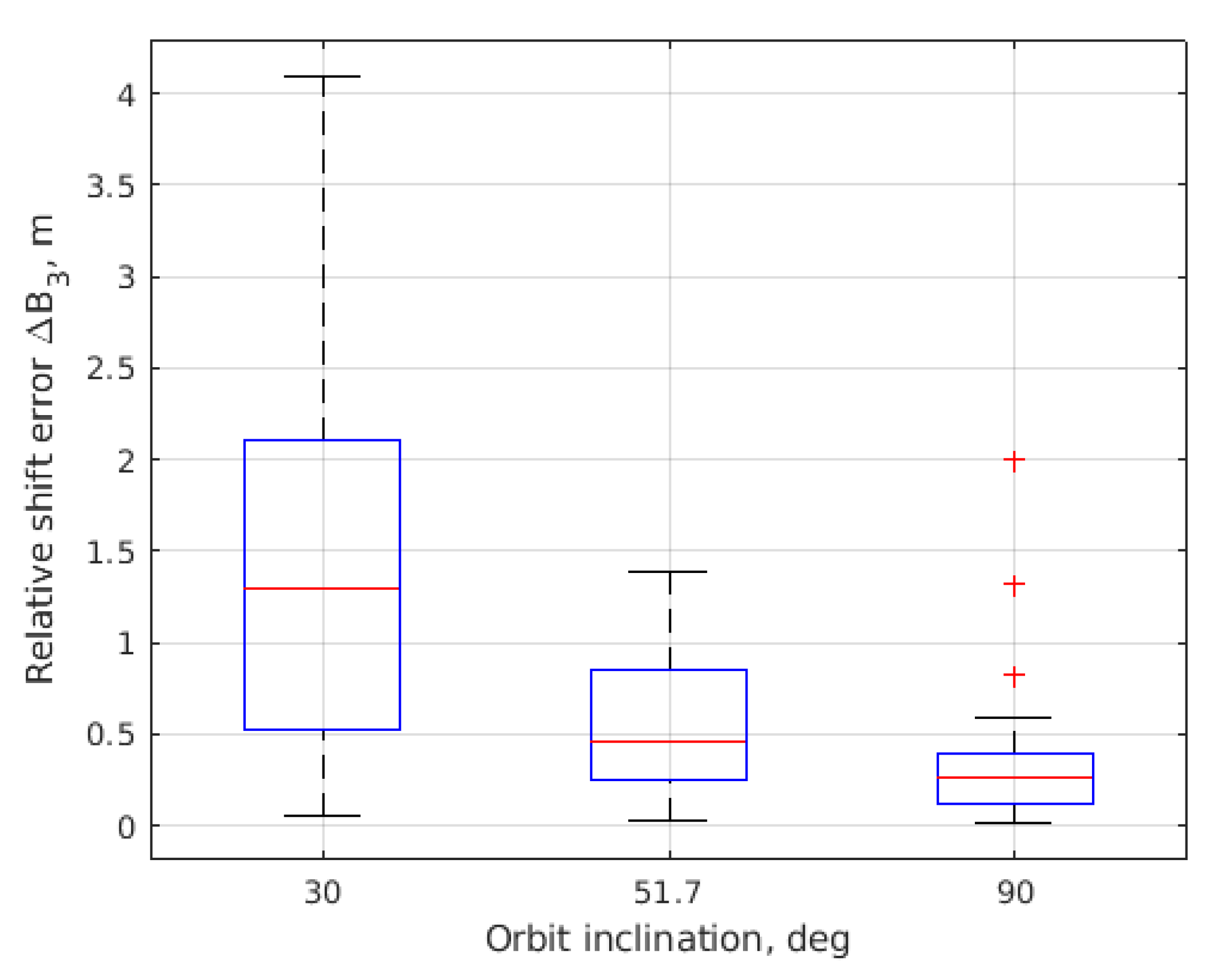
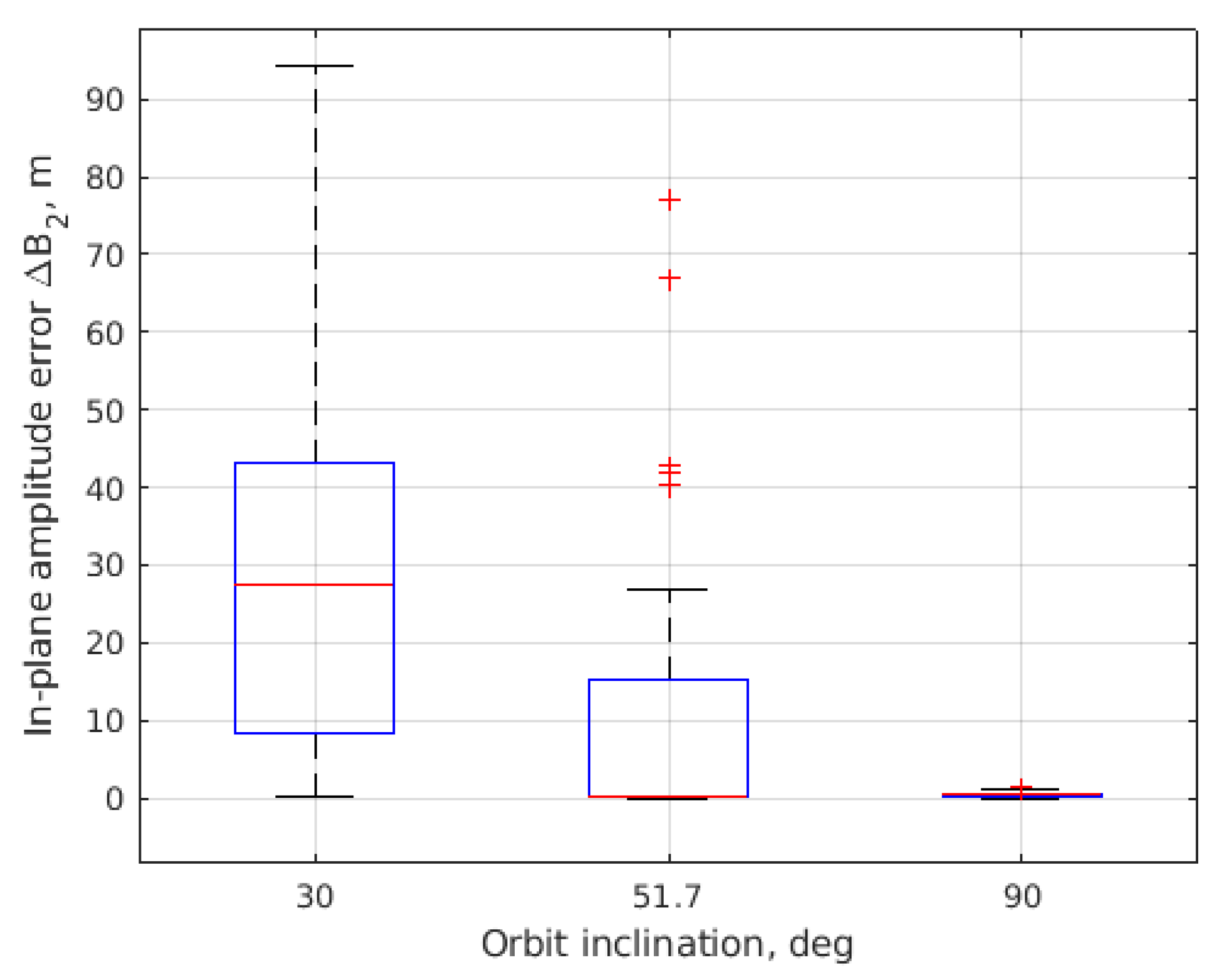
4. Results of Numerical Study
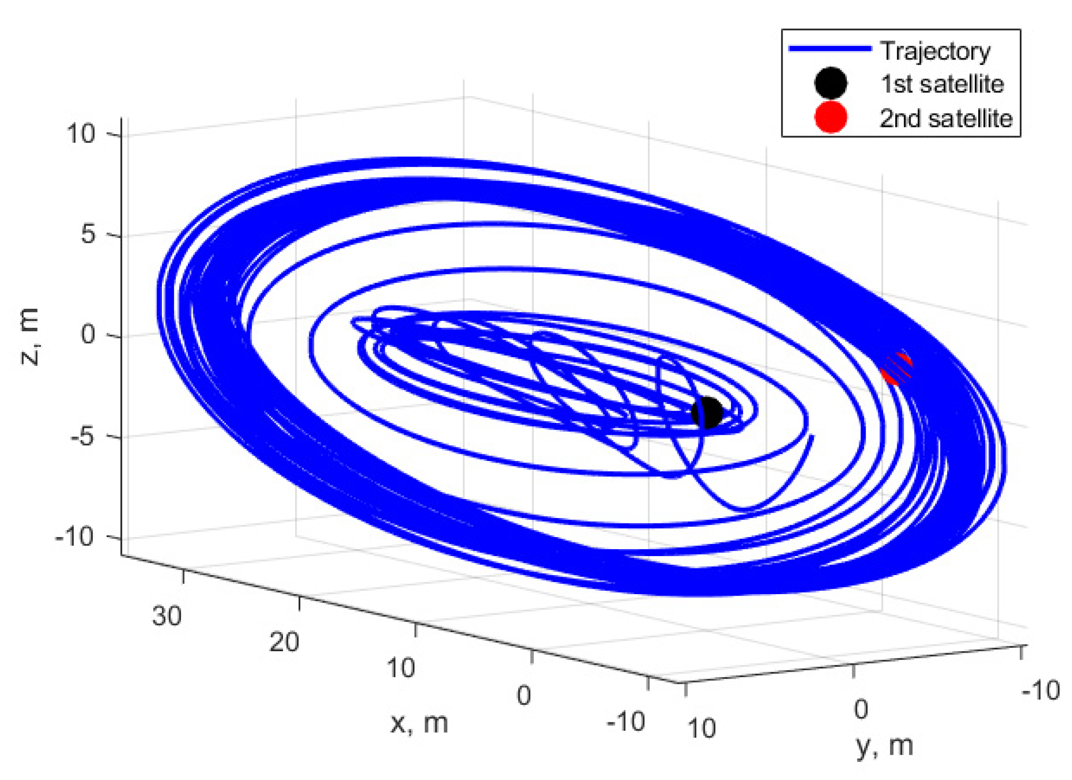
4.1. Free Motion of Two Satellites
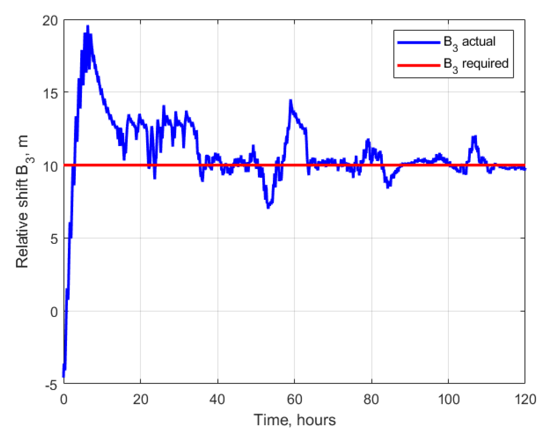
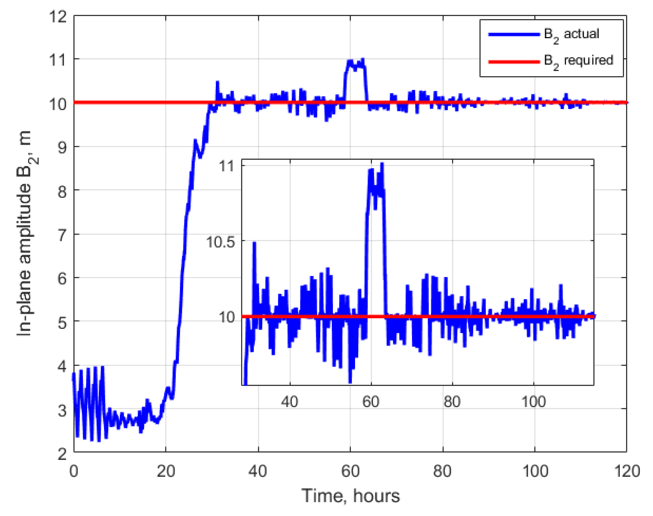
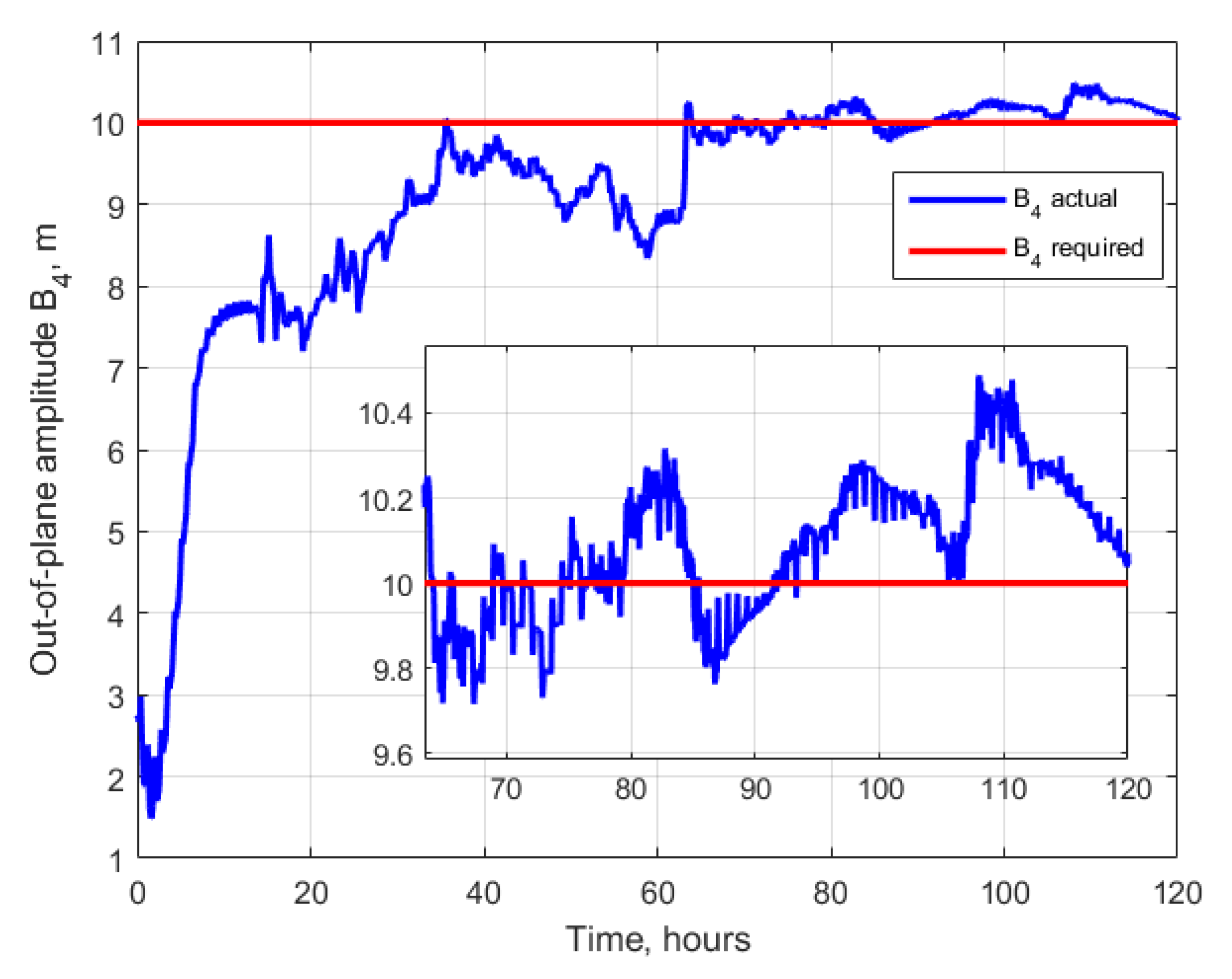
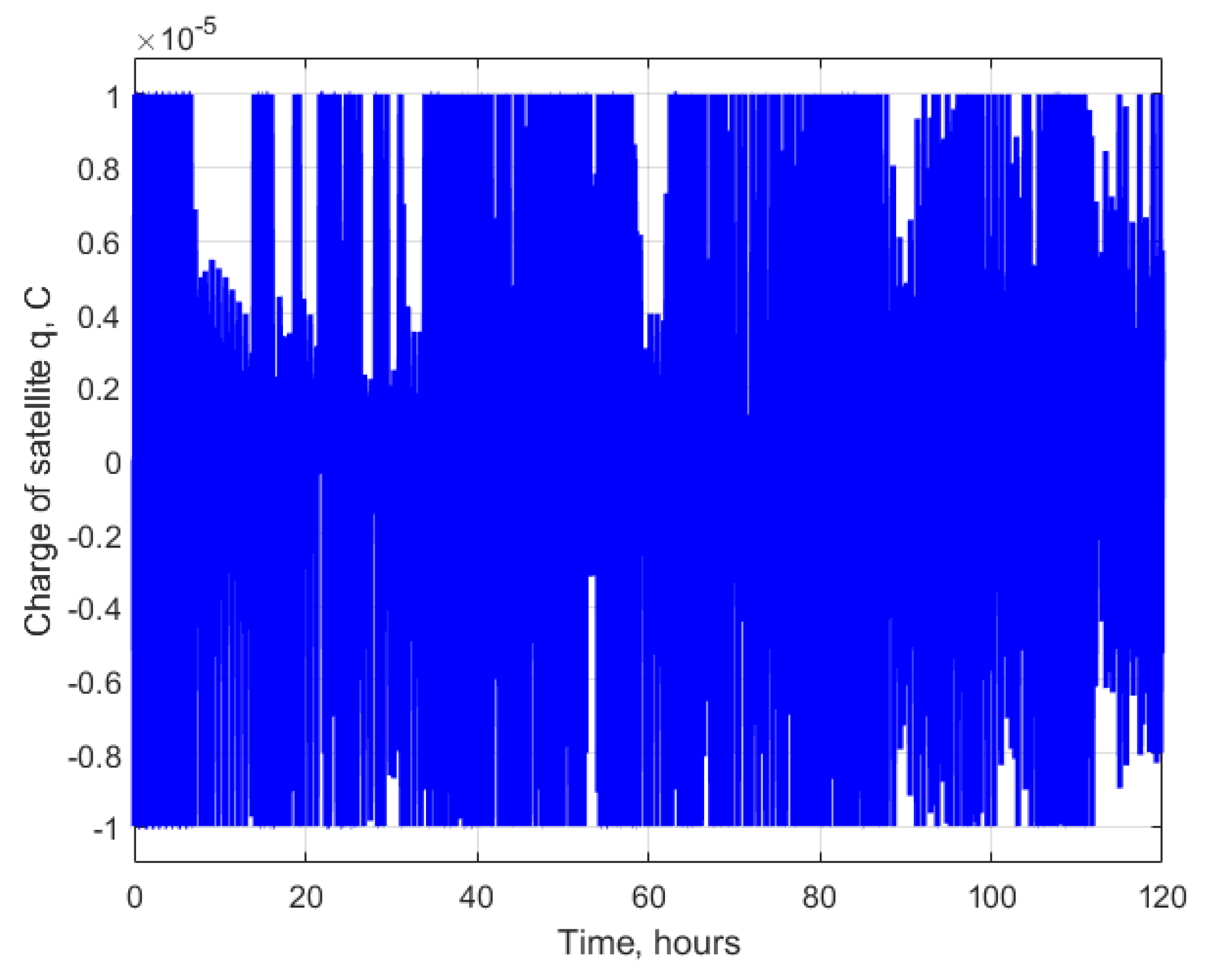
4.2. Case of Study of One Controlled Satellite
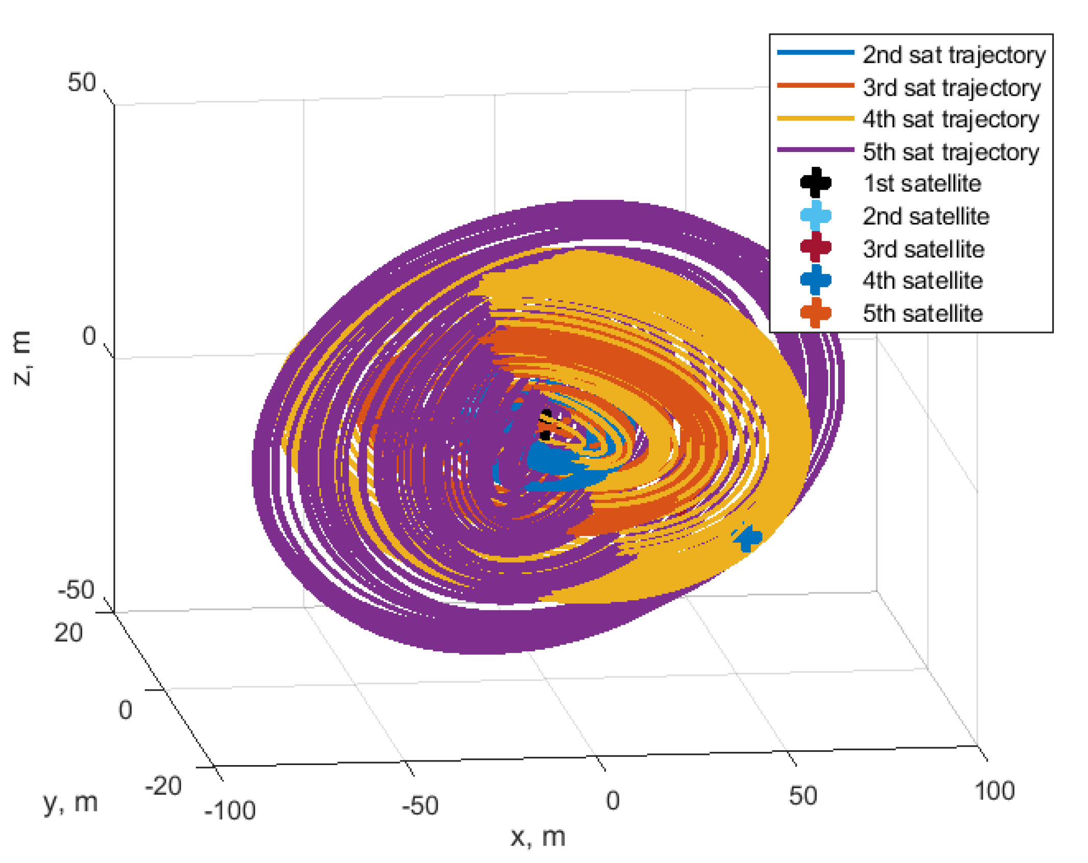
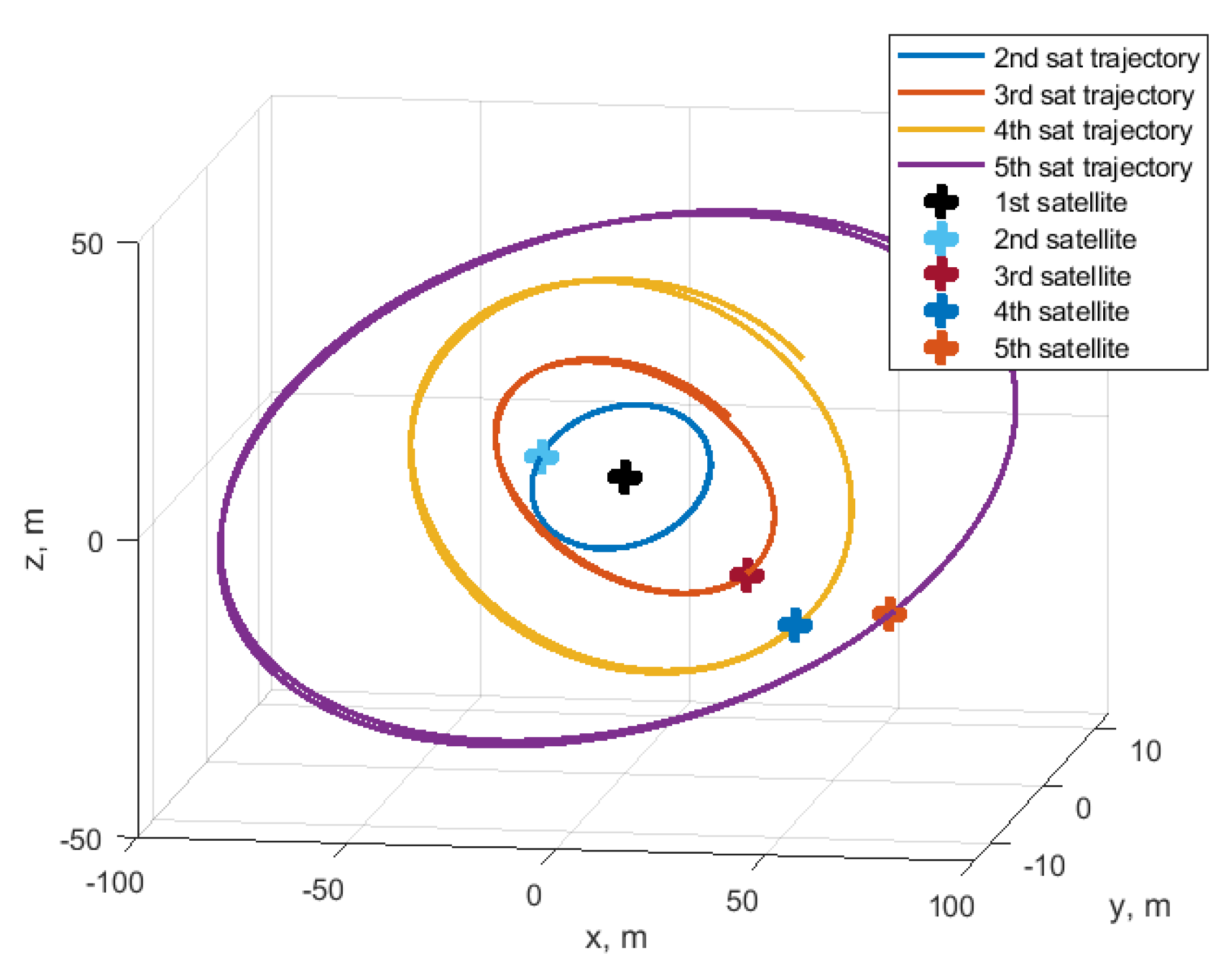
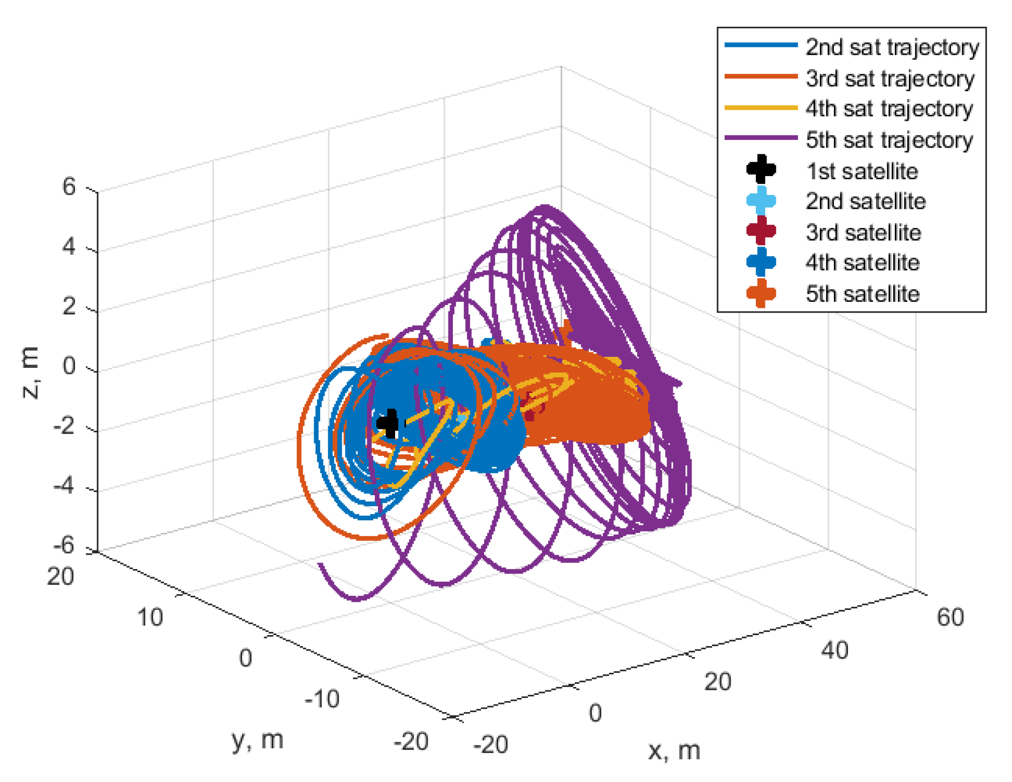
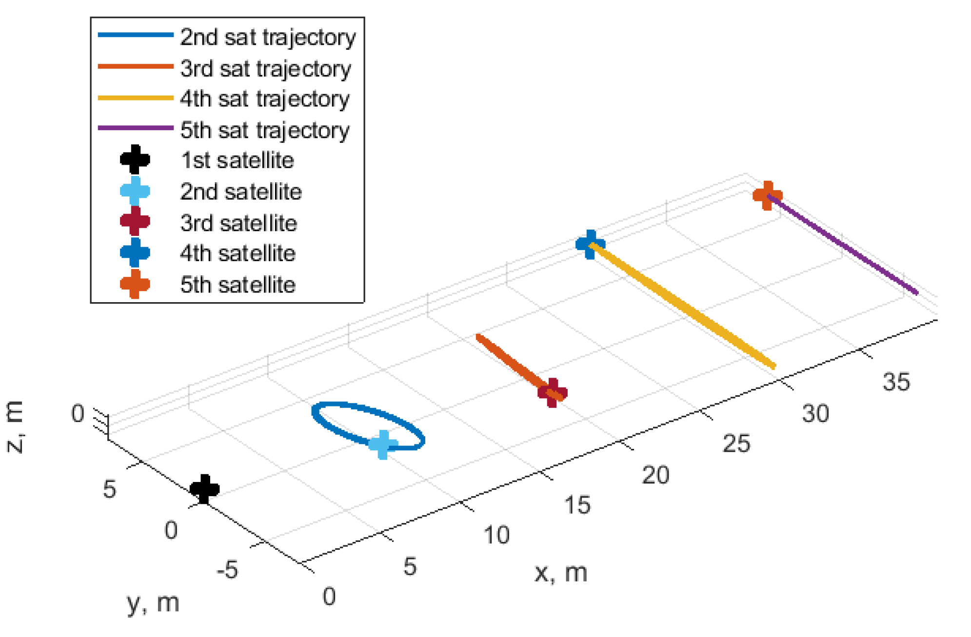
4.3. Cases of Satellites Swarm
4.3.1. Nested Ellipses
4.3.2. Train Formation
5. Conclusions
Author Contributions
Funding
Institutional Review Board Statement
Informed Consent Statement
Data Availability Statement
Conflicts of Interest
Notations
| LAO | Lorentz Augmented Orbit |
| LEO | Low Earth Orbit |
| CW | Clohessy–Wiltshire equations |
| LVLH | Local-Vertical/Local-Horizontal reference frame |
| Lorentz-force vector | |
| Satellite radius vector in Earth-centered inertial reference frame | |
| Satellite velocity in Earth-centered inertial reference frame | |
| Satellite charge | |
| Earth angular velocity | |
| Earth magnetic induction vector | |
| Radius of circular orbit | |
| Orbital angular velocity | |
| Vectors of the i-th satellite in the LVLH reference frame | |
| Relative position vector in the LVLH reference frame | |
| Control acceleration applied to i-th satellite | |
| Difference of the two control accelerations written in LVLH frame | |
| Relative motion parameters | |
| Earth magnetic dipole moment value | |
| Unit vector along the Earth’s dipole vector | |
| Distance from the Earth’s center of mass | |
| Unit vector along the satellite radius vector | |
| Angle between the magnetic south pole and geocentric north pole | |
| Latitude angle | |
| Greenwich’s longitude at initial time | |
| Deviation of motion parameters from the desired motion | |
| Desired motion parameters | |
| Lyapunov function | |
| Positive control parameters | |
| Parameters for control implementation | |
| Satellite mass | |
| Lorentz force vector components | |
| Value of the satellite charge | |
| Maximum value of the satellite charge | |
| Speed of the change in the satellite charge | |
| Simulation time step |
References
- Guzmán, J.J.; Edery, A. Mission design for the MMS tetrahedron formation. IEEE Aerosp. Conf. Proc. 2004, 1, 533–540. [Google Scholar] [CrossRef]
- Tzabari, M.; Holodovsky, V.; Shubi, O.; Eytan, E.; Altaratz, O.; Koren, I.; Aumann, A.; Schilling, K.; Schechner, Y.Y. CloudCT 3D volumetric tomography: Considerations for imager preference, comparing visible light, short-wave infrared, and polarized imagers. Proc. SPIE Polariz. Sci. Remote Sens. X 2021, 11833, 19–26. [Google Scholar] [CrossRef]
- Dauner, J.; Elsner, L.; Ruf, O.; Borrmann, D.; Scharnagl, J.; Schilling, K. Visual servoing for coordinated precise attitude control in the TOM small satellite formation. Acta Astronaut. 2022, 202, 760–771. [Google Scholar] [CrossRef]
- Mashtakov, Y.; Ovchinnikov, M.; Ivanov, D.; Roldugin, D.; Shestakov, S.; Klimov, P.; Iyudin, A.; Svertilov, S.; Pansyrnyi, O.; Churilo, I. Nanosatellites triangle formation flying for terrestrial gamma-ray flashes and transient luminous events study. In Proceedings of the International Astronautical Congress, IAC, 15 October 2020; International Astronautical Federation (IAF): Paris, France, 2020. [Google Scholar]
- Joffre, E.; Wealthy, D.; Fernandez, I.; Trenkel, C.; Voigt, P.; Ziegler, T.; Martens, W. LISA: Heliocentric formation design for the laser interferometer space antenna mission. Adv. Sp. Res. 2020, 67, 3868–3879. [Google Scholar] [CrossRef]
- Biktimirov, S.; Belyj, G.; Pritykin, D. Satellite Formation Flying for Space Advertising: From Technically Feasible to Economically Viable. Aerospace 2022, 9, 419. [Google Scholar] [CrossRef]
- Biktimirov, S.; Ivanov, D.; Pritykin, D. A satellite formation to display pixel images from the sky: Mission design and control algorithms. Adv. Sp. Res. 2022, 69, 4026–4044. [Google Scholar] [CrossRef]
- Kramer, A.; Bangert, P.; Schilling, K. UWE-4: First Electric Propulsion on a 1U CubeSat—In-Orbit Experiments and Characterization. Aerospace 2020, 7, 98. [Google Scholar] [CrossRef]
- Scharnagl, J.; Haber, R.; Dombrovski, V.; Schilling, K. NetSat—Challenges and lessons learned of a formation of 4 nano-satellites. Acta Astronaut. 2022, 201, 580–591. [Google Scholar] [CrossRef]
- Kahr, E.; Roth, N.; Montenbruck, O.; Risi, B.; Zee, R.E. GPS relative navigation for the CanX-4 and CanX-5 formation-flying nanosatellites. J. Spacecr. Rockets 2018, 55, 1545–1558. [Google Scholar] [CrossRef]
- Leonard, C.L.; Hollister, W.M.; Bergmann, E. V Orbital formationkeeping with differential drag. J. Guid. Control. Dyn. 1989, 12, 108–113. [Google Scholar] [CrossRef]
- Johnson, L.; Whorton, M.; Heaton, A.; Pinson, R.; Laue, G.; Adams, C. NanoSail-D: A solar sail demonstration mission. Acta Astronaut. 2011, 68, 571–575. [Google Scholar] [CrossRef] [Green Version]
- Hogan, E.A.; Schaub, H. Collinear invariant shapes for three-spacecraft Coulomb formations. Acta Astronaut. 2012, 72, 78–89. [Google Scholar] [CrossRef]
- Saaj, C.M.; Lappas, V.; Schaub, H.; Izzo, D. Hybrid propulsion system for formation flying using electrostatic forces. Aerosp. Sci. Technol. 2010, 14, 348–355. [Google Scholar] [CrossRef]
- Kwon, D.W. Propellantless formation flight applications using electromagnetic satellite formations. Acta Astronaut. 2010, 67, 1189–1201. [Google Scholar] [CrossRef]
- Ivanov, D.; Ovchinnikov, M. Constellations and formation flying. In Cubesat Handbook; Academic Press: Cambridge, MA, USA, 2021; pp. 135–146. [Google Scholar]
- Peck, M.A. Prospects and challenges for lorentz-augmented orbits. Collect. Tech. Pap.-AIAA Guid. Navig. Control Conf. 2005, 3, 1631–1646. [Google Scholar] [CrossRef]
- Schaffer, L.; Burns, J.A. Charged dust in planetary magnetospheres: Hamiltonian dynamics and numerical simulations for highly charged grains. J. Geophys. Res. Sp. Phys. 1994, 99, 17211–17223. [Google Scholar] [CrossRef]
- Saaj, C.M.; Lappas, V.; Richie, D.; Peck, M.; Streetman, B.; Schaub, H.; Izzo, D. Electrostatic Forces for Satellite Swarm Navigation and Reconfiguration; European Space Agency: Paris, France, 2006.
- Paul, S.N.; Frueh, C. Analytical expressions for orbital perturbations due to Lorentz force. Acta Astronaut. 2021, 182, 466–485. [Google Scholar] [CrossRef]
- Huang, X.; Yan, Y.; Zhou, Y. Dynamics and control of spacecraft hovering using the geomagnetic Lorentz force. Adv. Sp. Res. 2014, 53, 518–531. [Google Scholar] [CrossRef]
- Liao, H.; Xu, Y.; Zhu, Z.; Deng, Y.; Zhao, Y. A new design of drag-free and attitude control based on non-contact satellite. ISA Trans. 2019, 88, 62–72. [Google Scholar] [CrossRef]
- Zhang, Z.; Gong, S.; Li, J. Lorentz force time-optimal transfer trajectory design in Jovian magnetic field. Adv. Sp. Res. 2015, 55, 1061–1073. [Google Scholar] [CrossRef]
- Yamakawa, H.; Hachiyama, S.; Bando, M. Attitude dynamics of a pendulum-shaped charged satellite. Acta Astronaut. 2012, 70, 77–84. [Google Scholar] [CrossRef]
- Abdel-Aziz, Y.A.; Shoaib, M. Attitude dynamics and control of spacecraft using geomagnetic Lorentz force. Res. Astron. Astrophys. 2014, 15, 127–144. [Google Scholar] [CrossRef] [Green Version]
- Kalenova, V.I.; Morozov, V.M. Novel approach to attitude stabilization of satellite using geomagnetic Lorentz forces. Aerosp. Sci. Technol. 2020, 106, 106105. [Google Scholar] [CrossRef]
- Prabhat, H.; Mukherjee, B.K.; Giri, D.K.; Sinha, M. Fault-tolerant sliding mode satellite attitude stabilization using magneto-Coulombic torquers. Aerosp. Sci. Technol. 2022, 121, 107316. [Google Scholar] [CrossRef]
- Aleksandrov, A.Y.; Aleksandrova, E.B.; Tikhonov, A.A. Stabilization of a programmed rotation mode for a satellite with electrodynamic attitude control system. Adv. Sp. Res. 2018, 62, 142–151. [Google Scholar] [CrossRef]
- Peng, C.; Gao, Y. Lorentz-force-perturbed orbits with application to J2-invariant formation. Acta Astronaut. 2012, 77, 12–28. [Google Scholar] [CrossRef]
- Pollock, G.E.; Gangestad, J.W.; Longuski, J.M. Analytical solutions for the relative motion of spacecraft subject to Lorentz-force perturbations. Acta Astronaut. 2011, 68, 204–217. [Google Scholar] [CrossRef]
- Yamakawa, H.; Bando, M.; Yano, K.; Tsujii, S. Spacecraft relative dynamics under the influence of geomagnetic lorentz force. In Proceedings of the AIAA/AAS Astrodynamics Specialist Conference, Toronto, ON, Canada, 2–5 August 2010. [Google Scholar] [CrossRef]
- Tsujii, S.; Bando, M.; Yamakawa, H. Spacecraft Formation Flying Dynamics and Control Using the Geomagnetic Lorentz Force. J. Guid. Control. Dyn. 2013, 36, 136–148. [Google Scholar] [CrossRef]
- Huang, X.; Yan, Y.; Zhou, Y. Optimal spacecraft formation establishment and reconfiguration propelled by the geomagnetic Lorentz force. Adv. Sp. Res. 2014, 54, 2318–2335. [Google Scholar] [CrossRef]
- Sun, R.; Shan, A.; Zhang, C.; Jia, Q. Optimal spacecraft rendezvous using the combination of aerodynamic force and Lorentz force. Adv. Sp. Res. 2021, 67, 3583–3597. [Google Scholar] [CrossRef]
- Hill, G.W. Researches in Lunar Theory. Am. J. Math. 1878, 1, 5–26. [Google Scholar] [CrossRef]
- Mashtakov, Y.; Ovchinnikov, M.; Petrova, T.; Tkachev, S. Two-satellite formation flying control by cell-structured solar sail. Acta Astronaut. 2020, 170, 592–600. [Google Scholar] [CrossRef]
- Merkin, D.R. Introduction to the Theory of Stability; Springer: New York, NY, USA, 1997. [Google Scholar]
- Barbashin, E.A. On construction of Lyapunov functions for non-linear systems. In Proceedings of the Proc. First Congr. IFAK, Moscow, Russia; 1961; pp. 742–751. Available online: https://dl.acm.org/doi/abs/10.1016/j.automatica.2022.110411 (accessed on 28 November 2022).


| Initial conditions | |
| Initial relative drift, | rand([−0.5;0.5]) m |
| Initial relative position constants | rand([5;5]) m |
| Satellite parameters | |
| Mass of the satellites, | 1 kg |
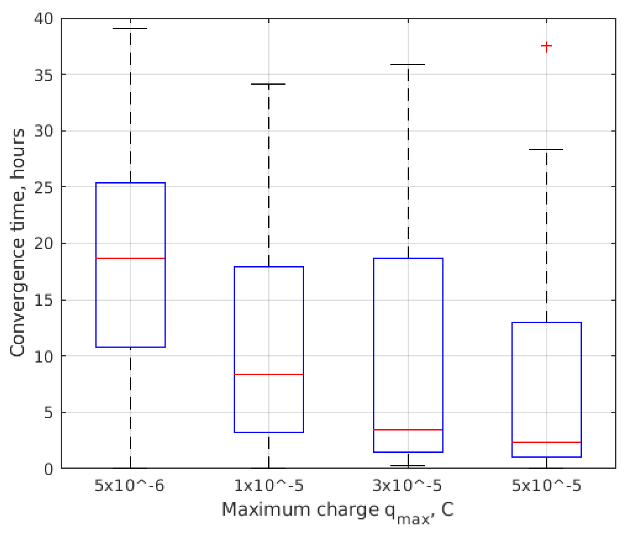
| Maximum charge, | 10 µC |
| Orbital parameters | |
| Altitude, | 500 km |
| Inclination, | 51.7° |
| Eccentricity, | 0 |
| Algorithms parameters | |
| Control gains | 10−6, 10−4 |
| Control gains | 10−6, 10−8, 10−7 |
| Maximal charge change rate , | 10−7 C/s |
| Required relative orbit parameters | [0, 10, 10, 10] m |
| Second stage algorithm threshold for and | 0.05 m, 2.5 m |
| Simulation step , s | 5 |
Disclaimer/Publisher’s Note: The statements, opinions and data contained in all publications are solely those of the individual author(s) and contributor(s) and not of MDPI and/or the editor(s). MDPI and/or the editor(s) disclaim responsibility for any injury to people or property resulting from any ideas, methods, instructions or products referred to in the content. |
© 2023 by the authors. Licensee MDPI, Basel, Switzerland. This article is an open access article distributed under the terms and conditions of the Creative Commons Attribution (CC BY) license (https://creativecommons.org/licenses/by/4.0/).
Share and Cite
Ivanov, D.; Amaro, G.; Mashtakov, Y.; Ovchinnikov, M.; Guerman, A. Formation Flying Lyapunov-Based Control Using Lorentz Forces. Aerospace 2023, 10, 39. https://doi.org/10.3390/aerospace10010039
Ivanov D, Amaro G, Mashtakov Y, Ovchinnikov M, Guerman A. Formation Flying Lyapunov-Based Control Using Lorentz Forces. Aerospace. 2023; 10(1):39. https://doi.org/10.3390/aerospace10010039
Chicago/Turabian StyleIvanov, Danil, Goncalo Amaro, Yaroslav Mashtakov, Mikhail Ovchinnikov, and Anna Guerman. 2023. "Formation Flying Lyapunov-Based Control Using Lorentz Forces" Aerospace 10, no. 1: 39. https://doi.org/10.3390/aerospace10010039