Article

Modelling of Parachute Airborne Clusters Flight Dynamics and Parachute Interactions

1
Key Laboratory of Aircraft Environment Control and Life Support, MIIT, Nanjing University of Aeronautics and Astronautics, Nanjing 210016, China
2
College of Aerospace Engineering, Nanjing University of Aeronautics and Astronautics, Nanjing 210016, China
3
Hongguang Airborne Equipment Company, Nanjing 210022, China
*
Author to whom correspondence should be addressed.
Aerospace 2023, 10(1), 51; https://doi.org/10.3390/aerospace10010051
Submission received: 31 October 2022 / Revised: 22 December 2022 / Accepted: 28 December 2022 / Published: 4 January 2023

Abstract

:
With the need for more condensed airborne clusters in a shortened time, there are increased risks of parachute collision and other interactions in the air. In this paper, the flight dynamics model of the parachute system is proposed for the whole deplaning airborne process, including parachute deployment, inflation, and the steady descent stages. The trajectories and velocities of the typical parachute airborne system are simulated, and the results are validated against the experimental measurement. To understand the potential interactions between parachutes, the flight dynamics of parachute airborne clusters, are then studied based on this model. The main parameters include the airborne altitudes, deplaning velocities, and airborne mass. The results show that the flight characteristics of parachutes are determined by the competence of the inertia effect and aerodynamic drags. The flight interactions of parachute clusters are most likely to occur at the moment of deployment, where the distance between parachutes is at a minimum. This critical distance increases with deplaning velocities and is insensitive to airborne altitudes. Adjusting the airborne order or using adaptive time periods by airborne mass can also avoid the potential interactions. The results of this paper can provide support for airborne strategies and help increase the safety and efficiency of airborne systems.

1. Introduction

Airborne systems play significant roles in both military and civil rescue. In the case of emergencies, there is an urgent need for more condensed airborne systems in a shortened time in the designated area. The mass of airborne systems can be significantly different, e.g., 70~140 kg per mission objectives, and the trajectories additionally vary a good deal. When the parachute airborne clusters deplane in shortened periods of time, there is a high risk that the parachutes may collide and twist into each other. At the Chicago Air Show in 2015, two skydivers collided into each other and this resulted in the failure of a parachute, leading to the death of young trooper [1]. Currently, we rely on the parachuters to control their flying directions, based on subjective judgement and experience, to avoid parachute interactions. In aerospace engineering, the gliding ratio, which is calculated as the ratio of lift to the aerodynamic drags, is commonly used to describe the travelling distance within certain airborne altitudes. However, the maneuvering ability of most round parachutes is limited, and their gliding ratio is commonly less than two while that of the parafoil is in the range of three to six [2]. Furthermore, because the parachute is made of flexible fabric, the flight performance is easily affected by winds [3,4,5]. Therefore, it is important to understand the trajectory and flight characteristics of parachute clusters in order to arrange proper airborne strategies and to avoid parachute interactions.
One common way to study the flight performance of a parachute is through flight tests where the velocities and trajectories of the whole deplaning and deceleration process can be recorded [6,7,8,9]. However, the results of flight tests are often affected by weather conditions and the results can vary significantly. Furthermore, the tests on interactions of the parachute clusters would unavoidably lead to the loss of parachuter and measurement devices. In the meantime, scholars have made progress in modelling the flight dynamics of parachutes numerically and have been able to provide quick and accurate predictions of parachute trajectories much more cheaply.
After the parachuter deplanes, the pilot parachute opens automatically to adjust the gesture and to stabilize. At the designated altitude, the main parachute is ejected from the assembly, and the lines and chute are then deployed in sequence by the pilot parachute. Once the main chute is fully deployed, the chute inflates with the high-speed air flow and forms a funnel shape. The inflated parachute increases the drag significantly and decelerates until reaching a steady speed before landing. To model the flight dynamics of parachute systems, the characteristics of the deployment, inflation and descent stages need to be analyzed individually due to their different physics.
In the parachute deployment stage, the folded parachute and lines pulled straight by the drag of the pilot parachute can be assumed as a tether system with nonuniform mass distribution. In the early 1970s, Toni [10] and Huckins [11,12] first proposed the dynamics model of line-first deployment to predict the parachute velocity and snatch force, respectively, where the pulling speed was assumed to be constant. Henrich considered the interaction force between the lines and the parachute bag and improved the model accuracy [13]. Mcveys and Wolf [14] further considered the density change during the deployment and their results showed that the snatch force was significantly affected by the parachute density. In these models, the deployed parachute was assumed to be straight, and the pilot parachute was in line with the parachuter as well as the parallel flow. To quantify the curving of the line system observed in the experiments, two-dimentional and three-dimentional flight dynamics models were developed where the lines were discretized as individual elements [15,16,17,18,19]. In these models, the line sail phenomenon of parachutes was predicted, which happens when the lines are sufficiently long.
During the inflation stage, the air flows in and the folded parachute expands outwards; in the meantime, the drag area increases significantly. The shape of the flexible chute is the complex result of the interaction between the decelerating flow and the transient shape; therefore, it is difficult to obtain the theoretical forms of the aerodynamic force precisely. Most scholars have developed semi-empirical dynamic models to investigate the load and trajectory of the parachute at the inflation stage, basing their findings on experimental measurements. Heinrich and Berndt performed wind tunnel tests to measure the transient parachute shape and load, respectively [20,21,22]. They proposed the inflation time model that the parachute shape could be expressed as a function of time and their prediction agrees well with the experiment results [23,24]. Scheubel and French proposed that the parachute distance during inflation was constant and that the inflation process could be expressed through this inflation distance [25,26]. This method was later developed for application in the Apollo mission, while much professional software was developed using this method [27]. Other methods of parachute inflation modelling also include the modelling of the radical equations; however the accuracy of these methods additionally depends on the empirical correlations from experiments [28]. New techniques of image processing assisted in the transient parachute shape detection in inflation and improved the accuracy of models [29,30,31]. In recent decades, scholars have started to use numerical methods to simulate the fluid–structure interaction behavior to predict the parachute shape. However, due to the expensive cost of coupling, semi-empirical dynamic models are still widely used in the rapid prediction of parachute trajectories [32,33].
In this paper, the whole deplaning process of parachute clusters is carefully examined, including the parachute deployment, inflation and descent stages. The flight dynamics equations were modelled, and the flight dynamics models of the parachute clusters were developed. Based on the model, the parachute trajectories as well as parachute velocities were calculated with the 4th Runge–Kutta method. The simulation results match the experimental data well, indicating that the model is capable of providing quick and accurate predictions of trajectories of the parachute airborne clusters. Subsequently, the flight characteristics of the parachute systems were studied under different flight conditions and airborne mass. The potential interactions between parachutes were also investigated and the critical distance for interactions was proposed. The effect of airborne altitude, deplaning velocity, and airborne mass on the parachute interactions was then studied and strategies were proposed to reduce the potential risks from the parachute interactions. The results can provide evidence for airborne management and improve airborne safety. Furthermore, the results reveal the possibility of parachute interactions in the air and are significant for future research on similar topics.

2. Models and Equations

2.1. Deployment Stage

The motion of the parachute and parachuter are solved using the line-first deployment method, which is commonly deployed in aerospace applications. As shown in Figure 1, the parachute system is modelled as a pilot parachute, the parachute bag, the parachuter and the deploying main chute.
Here, θ is the flight path angle, m is the mass, Q = 1 2 ρ v 2 ( C A ) is the aerodynamic drag, where C A is the aerodynamic drag area. The subscripts w, ys, e, and v denote the parachuter, the pilot parachute, the deployed chute and the packed chute. F L and F L , D are the snatch force and the deployment drag force, respectively.
Assuming that the parachute system keeps straight in the flight direction, without wind interference, and that the elastic elongation of parachute systems is ignored, the system can be simplified as three particle units with a changing mass: the pilot parachute and the chute in the bag, the deploying chute, and the parachute with the deployed main chute. The equations of motion can be established in the coordinate of the flight path as:
{ d v w d t = g sin θ ( Q w + F L m w + m s , e ) d v y s d t = g sin θ ( Q y s F L , D m y s + m s , v )
F L and F L , D follow the correlation:
F L = m ( v w v y s ) 2 + F L D = m v 2 R + F L D
where m is the linear density of the parachute (it should be noted that the linear density is at its maximum at the nominal diameter D 0 ). v R is the relative speed between the pilot parachute and parachuter, which increases until the total system length L 0 is reached and the chute is fully deployed.

2.2. Inflation and Descent Stages

In the inflation and descent stages, there is no relative motion between the parachute and parachuter, and the parachute-parachuter system can be assumed to move at the same velocity. Assuming that there are no winds and that the aerodynamic lift force of the round parachute is negligible, the position of the center of mass of the chute does not change during inflation. Based on [25,26], the motion of the parachute systems can be expressed through the inflation distance, which is constant. As shown in Figure 2, the equation of motion in the coordinate of the flight path can be given as:
d v d S = 1 v [ g sin θ + 1 m w ( F k + Q w ) ]
Here, S is the distance of the parachute pass. The dynamic load F k is:
F k = ( m s + m f ) v d v d S + Q s + v d m f d t + m s g sin θ
Here, m f is the added mass and the subscript s denotes the main chute. The drag area of the parachute during inflation is dependent on the inflation distance [25,26].
( C A ) s = { k 1 S 0 S S 1 k 1 S + β ( S S 1 ) 4 S 1 < S S m ( C A ) 0 S m S
where, S 1 and S m are the inflation distances at the initial stage and when the parachute is fully inflated, k 1 and β are constant coefficients, and ( C A ) 0 is the nominal aerodynamic drag area.

2.3. Model Validations

To validate the accuracy of the current flight dynamics model, the parachute deployment and inflation process is simulated per the test conditions in [23,34]. The geometric and flight parameters are selected as identical to the experiment conditions shown in Table 1.
The deployment process is simulated with the same deplaning velocity as in [34] and the deployed velocity is compared in Figure 3. The simulated deployed velocity increases linearly with the deplaning velocity due to the stronger inertia; this is consistent with the results in the literature. Compared with the literature results, the current model in this paper can predict the parachute velocity within an error of 7.5%, indicating that the model accuracy is acceptable.
The inflation process in [23] is simulated and the transient deceleration process is compared in Figure 4. The simulated velocity matches the results well and the model successfully predicts that the deceleration is more efficient as the parachute inflates. The parachute fully inflates at a speed of 24.7 m/s numerically, compared with 22.9 m/s in the experiment, and the velocity error is 7.8%. This shows that the model is capable of predicting the transient parachute aerodynamic performance and its velocities during the inflation stage.

3. Flight Characteristics of Parachute Systems

3.1. Parachute and Flight Parameters

To further investigate the flight characteristics of the airborne clusters, a typical airborne scenario is studied with the aforementioned model. Each parachute system is equipped with a main chute with a nominal diameter of 11.7 m and a pilot parachute. Each line of parachute is 8.0 m long. The aerodynamic drag areas of the main chute and the pilot parachute are 0.95 m2 and 90 m2, respectively. The effect of airborne altitudes, deplaning velocities and airborne mass is investigated and the airborne conditions are shown in Table 2. The parameters are selected based on the common range of airborne experiments using a variable-controlling approach.

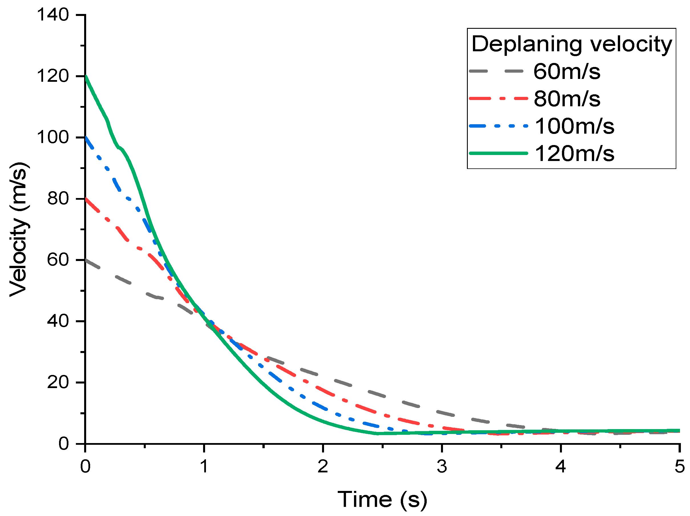
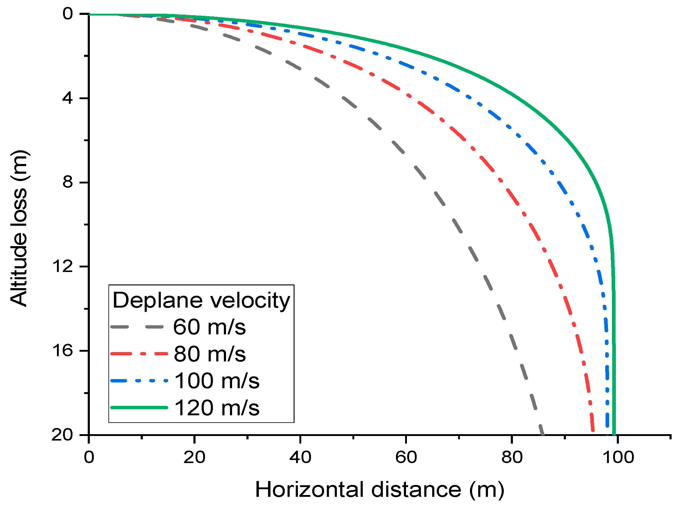
3.2. Effect of Flight Conditions

The air density varies at different airborne altitudes. Compared with 1000 m, the air density drops by 25% at 4000 m and this reduces the aerodynamic drags. The velocity changes and the trajectories of single parachute systems are shown in Figure 5 and Figure 6, respectively. At all altitudes, the parachute fully deploys at around 0.3 s and then starts to inflate. With the increase in the airborne altitudes, the velocity is slightly greater due to smaller drags. Compared with the airborne altitude at 1000 m, the inflation velocity increases by 4.7% at 4000 m. This velocity difference at different altitudes increases when the main chute inflates, which increases the aerodynamic drag area dramatically. After the parachute fully inflates, the parachute system reaches a steady descent where the velocities are similar. As a result, the horizontal distance of the airborne system increases with the airborne altitudes especially at the inflation stage, as shown in Figure 6. The horizontal distance increases by 6.1% at 4000 m, especially at the parachute inflation stage. It should be noted that the trajectories at different altitudes resemble each other and are nearly flat before full deployment. This is because the aerodynamic force of the pilot parachute is much smaller than the gravity and the inertia effect dominates the motion.
The flight velocity changes at different deplaning velocities are shown in Figure 7. With the increase in the deplaning velocities, the deceleration effect of the parachute is more significant as the drag increases with the square of velocities. The velocity difference between parachute systems decreases before the parachute inflates. As the parachute fully inflates, the order of parachute velocities reverses after ~1.0 s. This is because both deployment time and inflation time decrease due to the larger inertia. Compared with the system deplaning at 60 m/s, the deployment time and inflation time of the system deplaning at 120 m/s reduce by 53.3% and 42.7%, respectively. Therefore, the larger the deplaning velocities are, the earlier the parachute systems reach a steady state. The flight trajectories at different deplaning velocities are shown in Figure 8. The increase in the deplaning velocity directly increases the horizontal distance of the motion, e.g., the parachute systems deplaning at 120 m/s travel 15.9% 6further. Furthermore, the altitude loss during the parachute inflation reduces, as the parachute inflation time reduces. This explains the sharp “brake” at 120 m/s in the flight trajectories in Figure 8.

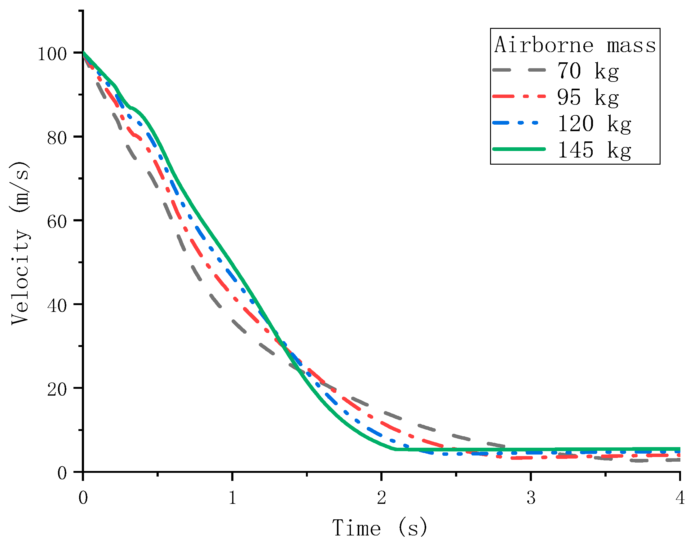
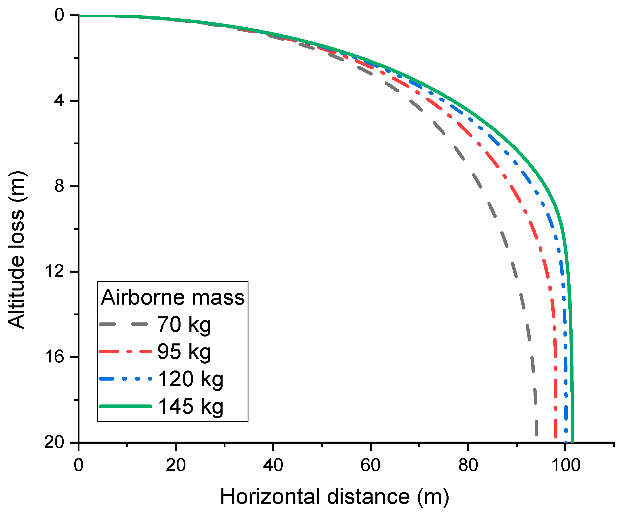
3.3. Effect of Airborne Mass

In the civil rescue event, it is common that different parachute airborne systems are equipped with different devices; therefore, the mass varies. The flight velocities of parachute systems with different masses are compared in Figure 9. The larger mass increases the inertia of the parachute systems and delays the deceleration process while the drag is independent of the mass. As a result, the velocity of the system with a larger mass is greater before the parachute inflates. However, the larger velocity reduces the inflation time as the inflation distance is constant and the parachute reaches a steady descent earlier. Compared with the system deplaning at 60 m/s, the deployment time and inflation time of the system deplaning at 120 m/s reduce by 53.3% and 42.7%, respectively. This results in the similar reversed velocity trend in Figure 9 as observed in Figure 7. It should be noted that the steady velocity is slightly higher for systems with a larger mass. The flight trajectories of the parachute systems with different masses are shown in Figure 10 and the results show that heavier parachute systems can travel 8.0% further in the horizontal direction. The effect of increasing the airborne mass is similar to increasing the deplaning velocity because both of them increase the inertia effect. However, the trajectories before inflation resemble each other as the minor velocity difference during deployment has a negligible effect on the aerodynamic drags.

4. Interactions of Airborne Clusters

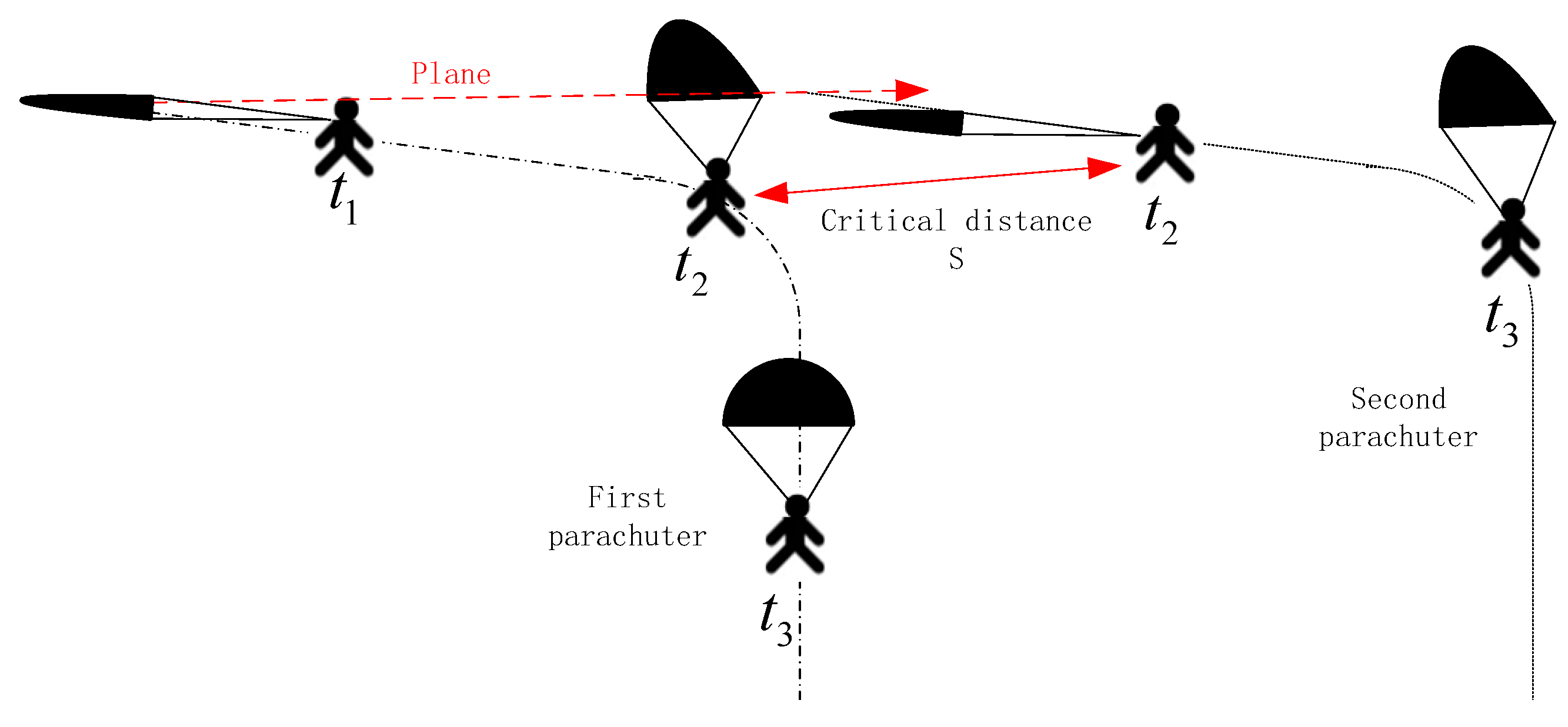
4.1. Criteria of Parachute Interactions

For typical airborne scenarios, the parachuter deplanes in one queue consequently or two queues alternately, which has been more common in recent decades. In this deplaning process, the two lines stand at the two sides of the rear exit and the parachuter in each line leaves in turn after one from another line. Assuming the pilot parachute opens and initiates the deployment process automatically and maneuvers are not considered during the airborne process, each parachuter deplanes at the same speed as the plane. Figure 11 shows the relative locations of two adjacent parachute systems after deplaning. As discussed in Section 3, with the deployment and inflation of the main chute, the horizontal velocity reduces due to the aerodynamic drag and the vertical velocity increases due to the gravity. In this process, the distance between the current parachute system and the last one continues to increase, especially when the parachute inflates. Once the parachute systems reach steady descent, the distance between adjacent parachute systems remains constant (t3 in Figure 11). However, at the deployment stage, the parachute and lines are released from the parachute pack in short time and increase the potential for parachute interactions. Therefore, the critical interactions between parachute systems are most likely to occur when the second parachute system deploys and the system length first reaches its maximum (t2 in Figure 11).
When the adjacent parachute systems are close in distance, the parachutes may collide with each other and fail to inflate. Because the parachute is made of flexible fabric, its motion is easily affected by the surrounding flow. Therefore, the critical distance for interactions (safety distance) can be estimated from the parachute shape at critical moment t2 in Figure 11 as follows:
S = D 0 / 2 + L 0
Here, the two items are the effective system diameters of the last parachute system (parachute inflated) and the current parachute system (parachute deployed), respectively. The parachute interactions are likely to occur when the critical distance (at the t2 moment) is smaller than this safety distance and the parachute motion is disturbed by a sudden airflow.

4.2. Airborne Conditions

To investigate the effect of airborne conditions on the parachute interactions, the typical two-queue airborne clusters deplaning from the rear exit are studied. The parachute parameters of each airborne system are the same as those in Section 3 and the safety distance can be estimated as from 13.85 m from Equation (6). The interval in the airborne clusters is 0.4 s and the width of the rear exit is 2.5 m. The main airborne parameters include airborne altitudes, deplaning velocities, and the mass arrangement of the airborne clusters (in a pair of parachute systems). The detailed airborne conditions are listed in Table 3.

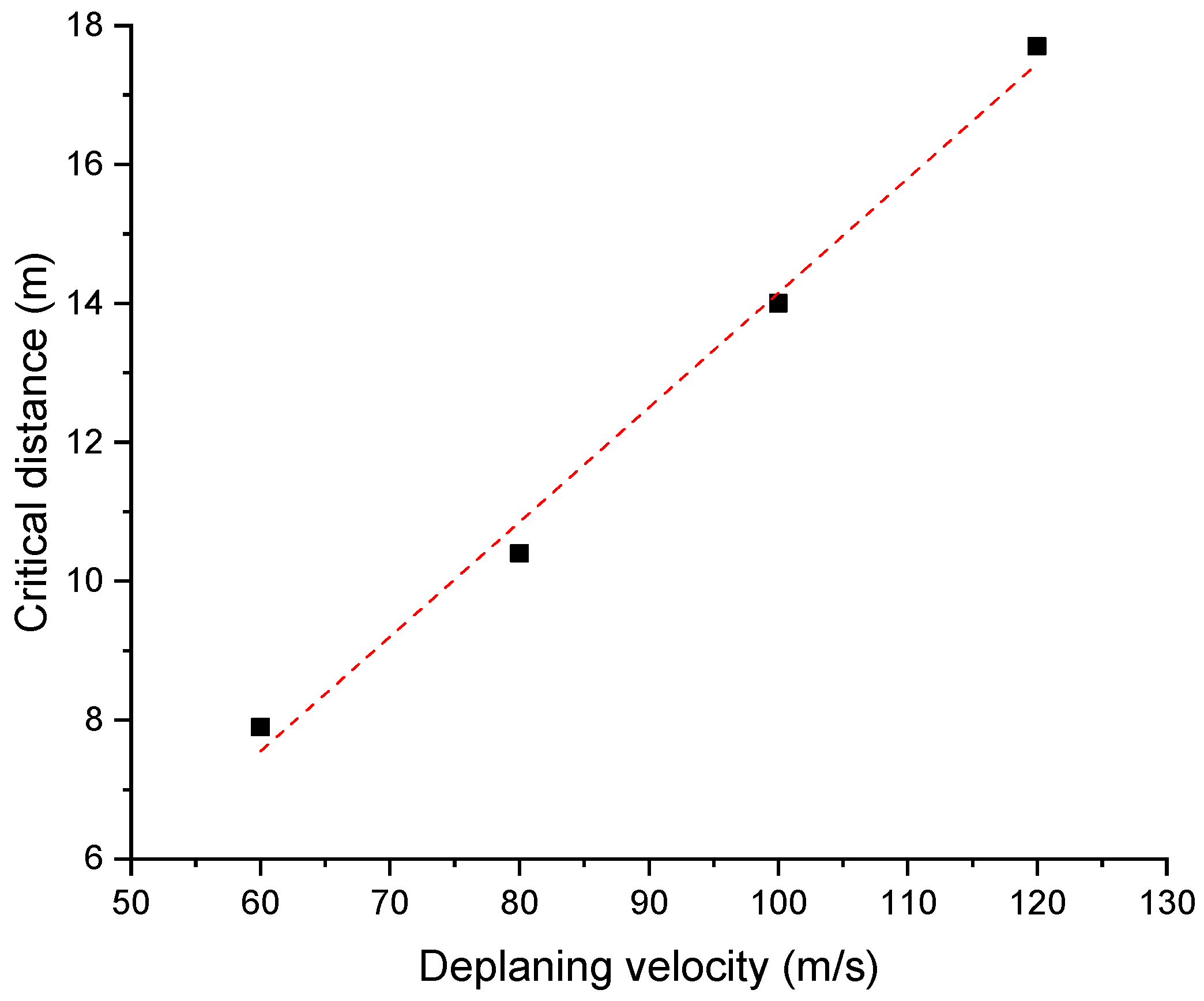
4.3. Effect of Flight Conditions

The critical distances between the parachute systems are calculated based on the trajectories of the airborne clusters. Figure 12 shows the critical distances at different airborne altitudes. As the airborne altitude increases, the decreased air density leads to smaller aerodynamic drags. The inertia effect dominates over the aerodynamic force and the parachute tends to maintain its motion. As a result, with the decrease in the airborne altitude, the critical distance between the parachute systems increases almost linearly. It should be noted that although the altitude reduces by three-quarters, the critical distance only increases by 16.4%, and is still in the risk region. However, deplaning at lower altitudes benefits a precise landing in condensed airborne clusters. Therefore, it may be favorable to choose the smallest airborne altitude possible.
The critical distances between parachute systems at different deplaning velocities are shown in Figure 13. The increase in the deplaning velocity increases the aerodynamic force dramatically and the aerodynamic deceleration dominates the inertia effect. Therefore, the parachutes decelerate more efficiently and the critical distance increases almost linearly with the deplaning velocities. In Figure 13, once the deplaning velocity is greater than 100 m/s, the airborne clusters are likely to be safe from parachute interactions. However, the larger deplaning velocity promotes the scattering of the landing location and should be selected based on the maneuverability of the parachutes.

4.4. Effect of Airborne Sequence

As discussed in Section 3.3, the flight trajectories of parachute systems vary with the airborne mass. Therefore, it is reasonable that a good arrangement of the airborne order by mass can reduce the possibility of parachute interactions. The critical distances with different airborne mass arrangements are shown in Figure 14. The increase in the airborne mass promotes the inertia effect; thus, the parachute system tends to maintain its motion. The motion of the first parachute system reduces the critical distance while that of the second parachute system increases the distance. Therefore, the critical distance decreases with the mass of the first parachute systems but increases with the mass of the second parachute systems. At the critical moment (t2 moment in Figure 11), the first parachute system is at the inflation stage and the second parachute system is still at the deployment stage where the aerodynamic force is much smaller than the gravity. This explains why the critical distance is relatively insensitive to the mass of the second parachute system. In real scenarios, it would be beneficial to arrange the airborne order by mass, e.g., postponing the heavy parachute systems. Furthermore, adopting adaptive time periods based on the mass of the last parachute system can also help. Longer airborne intervals after the heavy airborne systems lead to larger critical distances and hence help to avoid parachute interactions.

5. Concluding Remarks

In this paper, the flight dynamics model of parachute airborne clusters was established, and the flight characteristics of parachute systems were studied to investigate the interactions between parachutes. To achieve this, the general characteristics of single parachute systems were studied first, and the effect of airborne conditions and airborne mass was examined. Based on this, the critical distances between adjacent parachute systems were studied. The main conclusions include:
1. After the parachute system deplanes, its horizontal velocity decreases due to aerodynamic force and vertical velocity increases due to gravity. The flight trajectory is dominated by the competence of the inertia effect and aerodynamic accelerations.
2. The increase in the deplaning velocity and decrease in the airborne velocity increase the aerodynamic drags and hence the horizontal distance decreases. The increased airborne mass promotes the inertia effect; as a result, the parachute system tends to maintain its motion and move further horizontally.
3. The critical distance for interactions occurs at the moment of deployment when the parachute system length reaches its maximum. To avoid parachute interactions, the critical distance between parachutes should be kept greater than the effective length of adjacent parachute systems.
4. This critical distance is affected mostly by the flight characteristics of the first parachute system. The critical distance increases at smaller airborne altitudes and greater deplaning velocities. However, the selection of airborne conditions needs to consider the concentration of landing locations.
5. The arrangement of the airborne order based on mass, e.g., postponing the heavy parachute systems, can reduce the risks of parachute interactions. Adaptive airborne intervals should be adopted with longer intervals after the heavy systems.

Author Contributions

Conceptualization, J.L. and L.Y.; methodology and software, C.Q.; formal analysis, Y.L. and C.Q.; writing—original draft preparation, Y.L. and C.Q.; writing—review and editing, Y.L., C.Q. and L.Y.; supervision, J.L. and L.Y.; project administration, J.L. and L.Y. All authors have read and agreed to the published version of the manuscript.

Funding

This research was funded by the Chinese National Natural Science Foundation (Grant No. 11972192).

Data Availability Statement

The data that support the findings of this study are available from the authors upon reasonable request.

Acknowledgments

The numerical computations were performed on Hefei advanced computing center.

Conflicts of Interest

The authors declare no conflict of interest.

References

  1. Devlin, K. Army Skydiver Dies after Airshow Accident, CNN, 18 August 2015. Available online: https://wsvn.com/news/army-skydiver-dies-after-airshow-accident/amp/&ved=2ahUKEwi52t2_hIb7AhVxj2oFHdaxCYUQFnoECB0QAQ&usg=AOvVaw1I0etLe6fxRQD31Ec0SS1c (accessed on 30 October 2022).
  2. Wuest, M.R.; Benney, R.J. Precision Airdrop; The Research and Technology Organisation (RTO) of NATO: Natick, MA, USA, 2005. [Google Scholar]
  3. Zhang, S.; Yu, L.; Wu, Z.; Jia, H.; Liu, X. Numerical investigation of ram-air parachutes inflation with fluid-structure interaction method in wind environments. Aerosp. Sci. Technol. 2021, 109, 106400. [Google Scholar] [CrossRef]
  4. Pirson, J.; Verbiest, E. A study of some factors influencing military parachute landing injuries. Aviat. Space Environ. Med. 1985, 56, 564–567. [Google Scholar] [PubMed]
  5. Goodrick, T. Estimation of wind effect on gliding parachute cargo systems using computer simulation. In Proceedings of the AIAA Aerodynamic Deceleration Systems Conference, Dayton, OH, USA, 14–16 September 1970. [Google Scholar]
  6. Boustani, J.; Cadieux, F.; Kenway, G.; Barad, M.; Kiris, C.; Brehm, C. Fluid-structure interaction simulations of the ASPIRE SR01 supersonic parachute flight test. Aerosp. Sci. Technol. 2022, 126, 107596. [Google Scholar] [CrossRef]
  7. Bendura, R.J.; Lundstrom, R.R.; Renfroe, P.G.; Lecroy, S.R. Flight Tests of Viking Parachute System in Three Mach Number Regimes. 2: Parachute Test Results; NASA Langley Research Center: Hampton, VA, USA, 2013. [Google Scholar]
  8. O’Farrell, C.; Sonneveldt, B.S.; Karhgaard, C.; Tynis, J.A.; Clark, I.G. Overview of the ASPIRE Project’s Supersonic Flight Tests of a Strengthened DGB Parachute. In Proceedings of the IEEE Aerospace Conference, Big Sky, MT, USA, 2–9 March 2019. [Google Scholar]
  9. Stein, J.M.; Madsen, C.M.; Strahan, A.L. An Overview of the Guided Parafoil System Derived from X-38 Experience. In Proceedings of the 18th AIAA Aerodynamic Decelerator Systems Technology Conference and Seminar, Munich, Germany, 23–26 May 2005. [Google Scholar]
  10. Toni, R. Theory on the dynamics of bag strip for a parachute deployment aided. In Proceedings of the 2nd AIAA Aerodynamic Deceleration Systems Conference, El Centro, CA, USA, 23–25 September 1968. [Google Scholar]
  11. Huckins, E.K. Techniques for Selection and Analysis of Parachute Deployment Systems; NASA Langley Research Center: Hampton, VA, USA, 1970. [Google Scholar]
  12. Huckins, E.K. Snatch force during lines-first deployments. J. Aircr. 1971, 8, 298–299. [Google Scholar] [CrossRef]
  13. Heinrich, H. A parachute snatch force theory incorporating line disengagement impulses. In Proceedings of the 4th Aerodynamic Deceleration Systems Conference, Palm Springs, CA, USA, 21–23 May 1973. [Google Scholar]
  14. McVey, D.; Wolf, D. Analysis of Deloyment and Inflation of Large Ribbon Parachute. J. Aircr. 1974, 11, 96–103. [Google Scholar] [CrossRef]
  15. Purvis, J. Prediction of parachute line sail during lines-first deployment. J. Aircr. 1983, 20, 940–945. [Google Scholar] [CrossRef]
  16. Eckroth, W.; Garrard, W.; Miller, N. Design of a recovery system for a reentry vehicle. In Proceedings of the Third International Conference on Adaptive Structures, San Diego, CA, USA, 9–11 November 1992. [Google Scholar]
  17. Yu, L.; Shi, X.; Yuan, W. Effects of Parachute Deployment Using Attached Apex Drogue. J. Nanjing Univ. Aeronaut. Astronaut. 2009, 41, 198–201. [Google Scholar]
  18. Tang, M.; Wang, L.; Liu, Y.; Zhang, S. Effects of Aerodynamics on Line Sail During Parachute Deployment. In Proceedings of the ASME 2021 Fluids Engineering Division Summer Meeting, Virtual, Online, 10–12 August 2021. [Google Scholar]
  19. Zhang, Q.; Cheng, W.; Peng, Y.; Qin, Z. A Multi-Rigid-body Model of Parachute Deployment. Chin. Space Sci. Technol. 2003, 23, 45–50. [Google Scholar]
  20. Heinrich, H. The Opening Time of Parachutes Under Infinite Mass Conditions. In Proceedings of the AIAA 6th Aerospace Sciences Meeting, New York, NY, USA, 22–24 January 1968. [Google Scholar]
  21. Heinrich, H.; Noreen, R. Analysis of parachute opening dynamics with supporting wind-tunnel experiments. J. Aircr. 1970, 7, 341–347. [Google Scholar] [CrossRef]
  22. Berndt, R.; Deweese, J. Filling Time Prediction Approach for Solid Cloth Type Parachute Canopies. In Proceedings of the 1st AIAA Aerodynamic Decelerator Systems Technology Conference, Reston, VA, USA, 7–9 September 1966. [Google Scholar]
  23. Heinrich, H.; Saari, D. Parachute opening shock calculations with experimentally established input functions. J. Aircr. 1978, 15, 100–105. [Google Scholar] [CrossRef]
  24. Wolf, D. A simplified dynamic model of parachute inflation. J. Aircr. 1974, 11, 28–33. [Google Scholar] [CrossRef]
  25. French, K. Initial phase of parachute inflation. J. Aircr. 1969, 6, 376–378. [Google Scholar] [CrossRef]
  26. Scheubel, F. Notes on Opening Shock of a Parachute; B.I.O.S. Interrogation Report No.104: London, UK, 1946. [Google Scholar]
  27. Taylor, A.; Murphy, E. The DCLDYN parachute inflation and trajectory analysis tool-an overview. In Proceedings of the 18th AIAA Aerodynamic Decelerator Systems Technology Conference and Seminar, Munich, Germany, 23–26 May 2005. [Google Scholar]
  28. Macha, J. A simple, approximate model of parachute inflation. In Proceedings of the Aerospace Design Conference, Irvine, CA, USA, 16–19 February 1993. [Google Scholar]
  29. Guo, P.; Xia, G.; Qin, Z.-z. Automated Image Measurement of Parachute Projection Area under Inflation Process. Procedia Eng. 2012, 29, 1944–1951. [Google Scholar] [CrossRef] [Green Version]
  30. Ghaem-Maghami, E.; Desabrais, K.; Johari, H. Measurement of the geometry of a parachute canopy using image correlation photogrammetry. In Proceedings of the 19th AIAA Aerodynamic Decelerator Systems Technology Conference and Seminar, Williamsburg, VA, USA, 21–24 May 2007. [Google Scholar]
  31. Johari, H.; Desabrais, K.; Lee, C. Effects of Inflation Dynamics on the Drag of Round Parachute Canopies. In Proceedings of the 19th AIAA Aerodynamic Decelerator Systems Technology Conference and Seminar, Williamsburg, VA, USA, 21–24 May 2007. [Google Scholar]
  32. Haitao, G.; Dong, S.; Wang, Y.; Qin, Z. Influence of Inflation Conditions Parachute Inflation. Chin. Space Sci. Technol. 2008, 6, 45–51. [Google Scholar]
  33. Ginn, J.M.; Clark, I.G.; Braun, R.D. Parachute dynamic stability and the effects of apparent inertia. In Proceedings of the AIAA Atmospheric Flight Mechanics Conference, Atlanta, GA, USA, 16–20 June 2014. [Google Scholar]
  34. National Defence Industry Press. Editorialteam, Introduction of Parachute Technology; National Defence Industry Press: Beijing, China, 1977. [Google Scholar]
Figure 1. Schematics of the parachute deployment process.
Aerospace 10 00051 g001
Figure 2. Schematics of the parachute inflation and descent process.
Aerospace 10 00051 g002
Figure 3. Comparison of parachute deployed velocity with literature.
Aerospace 10 00051 g003
Figure 4. Comparison of parachute velocity during inflation with literature.
Aerospace 10 00051 g004
Figure 5. Velocity changes of parachute systems at different altitudes.
Aerospace 10 00051 g005
Figure 6. Flight trajectories of parachute systems at different altitudes.
Aerospace 10 00051 g006
Figure 7. Velocity changes of parachute airborne systems at different deplaning velocities.
Aerospace 10 00051 g007
Figure 8. Flight trajectories of parachute airborne systems at different deplaning velocities.
Aerospace 10 00051 g008
Figure 9. Velocity changes of parachute systems with different masses.
Aerospace 10 00051 g009
Figure 10. Flight trajectories of parachute systems with different masses.
Aerospace 10 00051 g010
Figure 11. Relative locations of adjacent parachute systems at different moments.
Aerospace 10 00051 g011
Figure 12. Critical distances between parachute systems at different airborne altitudes.
Aerospace 10 00051 g012
Figure 13. Critical distances between parachute systems at different deplaning velocities.
Aerospace 10 00051 g013
Figure 14. Critical distances between parachute systems with different mass.
Aerospace 10 00051 g014
Table 1. Geometric and flight parameters of the parachute system.
Deployment Stage Inflation Stage
D 0 (m)10.6Parachute typeC-9 flat circle parachute
L 0 (m)15.49 D 0 (m)8.5
( C A ) y s (m2)0.3Deployed velocity (m/s)77
m w (kg)102.25 ( C A ) 0 (m2)45
Altitude, h (m)600 m w (kg)200
Altitude, h (m)1850
Table 2. Airborne conditions.
Airborne Altitude (m)Deplaning Velocity (m/s)Airborne Mass (kg)
1000, 2000, 3000, 400010095
100060, 80, 100, 12095
100010070, 95, 110, 130
Table 3. Airborne conditions of the clusters.
Mass Sequence of Parachute Systems (kg)Airborne Altitude (m)Deplaning Velocity (m/s)
90-901000100
2000
3000
4000
90-90100060
80
100
120
Mixed combinations of 70, 90, 120, 1451000100
Disclaimer/Publisher’s Note: The statements, opinions and data contained in all publications are solely those of the individual author(s) and contributor(s) and not of MDPI and/or the editor(s). MDPI and/or the editor(s) disclaim responsibility for any injury to people or property resulting from any ideas, methods, instructions or products referred to in the content.

