A High-Confidence Intelligent Measurement Method for Aero-Engine Oil Debris Based on Improved Variational Mode Decomposition Denoising

Abstract

This paper presents an effective method for measuring oil debris with high confidence to ensure the wear monitoring of aero-engines, which suffers from severe noise interference, weak signal characteristics, and false detection. First, an improved variational mode decomposition algorithm is proposed, which combines wavelet transform and interval threshold processing to suppress the complex noise interference on the signal. Then, a long-short-term memory neural network with deep scattering spectrum preprocessing is used to identify the signal characteristics under the multi-resolution analysis framework. The optimal hyperparameters are automatically configured using Bayesian optimization to solve the problem of weak, distorted, and hard-to-extract signal characteristics. Finally, a detection algorithm based on multi-window fusion judgment is applied to improve the confidence of the detection process, reduce the false detection and false alarm rate, and calculate the debris size information according to the sensor principle. The experimental results show that the proposed method can extract debris signals from noise with a signal-to-noise ratio improvement of more than 9 dB, achieve a high recognition accuracy of 99.76% with a missed detection rate of 0.24%, and output size information of debris to meet the need for aero-engine oil debris measurement.

1. Introduction

During the operation of an aero-engine, the relative movement and contact of mechanical parts on the surface generate friction and wear [1]. As the aviation engine operates for a long time, the wear will gradually increase, causing fatigue damage to mechanical parts and generating a large amount of metal debris distributed in the engine oil system, leading to engine performance degradation or functional and various other failures [2]. Therefore, detecting metal debris in the oil system can help evaluate the wear and health status of engine mechanical parts [3,4], avoid engine failures caused by mechanical part failure, and ensure the safe flight of aircraft.

Regular analysis of lubricating oil samples has become essential for accurate diagnosis and early detection of potential wear faults. Currently there are four leading technologies for detecting metal debris in oil systems [1]: optical [3,4], resistive–capacitive [5,6], acoustic [7,8], and electromagnetic [9,10]. The advantages and disadvantages are shown in

Table 1. Comparison of advantages and disadvantages of different measurement methods [1].

Methods	Advantages	Disadvantages
Optical	High precision; morphological information.	Low efficiency; affected by bubbles and oil transparency.
Resistive–capacitive	Simple structure; high measurement accuracy.	Cannot distinguish particle material and cause oil deterioration.
Acoustic	Distinguishes between bubbles and solid particles.	Cannot distinguish particle material; interference of flow speed, viscosity, vibration.
Electromagnetic	Significant flow rate and high efficiency; distinguishes between ferromagnetic and non-ferromagnetic particles.	Interference of vibration and electromagnetic noise; relatively low resolution.

.

Among them, the electromagnetic measurement is the most practical mechanical wear measurement method. It detects metal particles through a magnetic field composed of excitation and induction coils [9,10]. It can identify the source and degree of damage of the mechanical parts based on the waveform characteristics of the induced electromotive force [11]. However, in actual measurements, due to multiple sources of vibration interference and electromagnetic interference in the oil circulation system [12], the background noise is intense, and there are problems such as weak signals and waveform distortion [13,14]. With the traditional signal waveform recognition methods it is difficult to extract metal debris signal characteristics effectively [13], often resulting in missed and false measurements [15], leading to low accuracy. Therefore, current research on oil debris measurement mainly focuses on signal denoising and feature extraction [1].

Regarding signal denoising processing, current research often targets specific noise sources for processing. For example, (1) for the problem that low-frequency vibration noise affects debris measurement Fan et al. [15] proposed a time-invariant wavelet transform method to eliminate vibration noise. Li et al. [16] improved the oil debris measurement capability based on the wavelet domain information. Luo et al. [12] applied fractional calculus technology to extract oil particle characteristics from low-resonance components. (2) For electromagnetic noise interference Du et al. [4] optimized the structure of debris sensors to form a parallel LC (inductance–capacitance) resonance circuit with a unique resonance frequency. Li et al. [9] designed a parallel LCR (inductance–capacitance–resistance) resonance applied to each induction coil, significantly improving the sensor’s signal-to-noise ratio and sensitivity. (3) For background noise Zhu et al. [17] designed an integrated sensor comprising eight groups of miniature multiplexed sensing elements. Yu et al. [18] proposed a symplectic geometry mode decomposition (SGMD) to reduce or separate the noise. Some studies have tested fusion algorithms. For example, Bozchalooi et al. [19] used a two-stage denoising method. In the first stage, an adaptive sub-band filtering technology based on wavelets was applied to eliminate vibration-related interference. In the second stage, threshold setting was performed on the output of the adaptive filter to eliminate background noise, thereby improving the measurement accuracy of debris monitoring. The above research indicates that eliminating complex noise sources will be challenging if only one type of noise is processed and the coupling and superposition between different types of noise is ignored. Therefore, it is necessary to research fusion denoising algorithms.

Regarding signal waveform recognition and extraction, current research mainly adopts a threshold judgment method based on sensor signals. For example, Hong et al. [13] proposed a fractional calculus technology for debris signals in noisy environments, which can effectively detect small particle signals. Zhi et al. [11] separated the debris overlapping signals of the debris sensor through signal cross-processing. Hong et al. [20] used a piecewise function to describe the debris overlapping behavior and developed an optimized measurement strategy to reduce erroneous measurements. Wu et al. [21] proposed an approach based on multiple correlation windows to improve the sensitivity and adaptability of oil debris detections. In addition, Guo et al. [22] conducted a numerical signal analysis, and they obtained the relationship between pulse characteristics and particle status, providing a reference for further debris signal processing. Most of the above studies are based on the traditional detection algorithms of threshold judgment, which require a lot of logical judgment and switching. The portability and adaptability of the algorithms could be more robust, and a more intelligent and efficient method needs to be explored.

Regarding intelligent algorithms for wear debris detection, Hong et al. [23] used a neural network to establish a general correction framework, aiming to solve the modeling and adaptability problems of different sensors and further reduce the detection error. Furthermore, Li et al. [24,25] applied deep learning to detect fatigue damage of aero-engines, proving the application value of deep learning in wear prediction. Aydin et al. [26] compared the prediction ability of five different deep learning models for debris wear and determined the optimal neural network architecture. Li et al. [27] introduced the constitutive model into the aero-engine fatigue damage assessment model, and the results showed that the design of deep learning network architecture greatly impacted the model effect. Deng et al. [28] realized the automatic optimization of a deep learning model for engine fatigue assessment using a dynamic hybrid ant colony optimization algorithm. Mahmoodzadeh et al. [29] compared the effects of various optimization algorithms and selected the most suitable optimization method for neural network hyperparameters.

Considering the widespread problems of serious noise interference, difficulty extracting waveform features, and missed and inaccurate measurements in the current measurement of metal debris in aero-engine oil systems, this paper proposes a high-confidence measurement method. Firstly, in order to eliminate complex noise from different sources and improve the signal-to-noise ratio, this paper presents an improved VMD (variational mode decomposition) fusion denoising algorithm; that is, first filtering out part of the high-frequency noise through wavelet transform, then using the VMD algorithm to separate and reconstruct signals without vibration noise modes, and finally processing VMD’s IMFs (intrinsic mode functions) through an IT (interval threshold), eliminating low-power background white noise and achieving the goal of distributed removal of complex noise from different sources. Secondly, in order to extract weak feature information of metal debris signals, this paper first uses DSS (deep scattering spectrum) to clearly show the detailed information in the original signal under the multi-resolution analysis framework. Then it develops an LSTM (long-short-term memory) deep learning neural network based on this information to recognize debris characteristics. Moreover, it configures its hyperparameters through BO (Bayesian optimization) to achieve accurate extraction and classification of debris characteristics. Finally, in order to improve the confidence of the measurement process and realize the output of characteristic debris information, this paper proposes a multi-window information fusion measurement method and, based on the principle of electromagnetic sensors, clarifies the relationship between debris size characteristics and electromagnetic signal waveforms. This paper verifies the method’s effectiveness through simulation and oil system measurement experiments.

The main content of this paper is organized as follows. Section 2 first describes the principle of the improved VMD-based fusion denoising algorithm. Section 3 expounds on the measurement method based on DSS-LSTM for oil debris signals. Section 4 shows the principle of the high-confidence measurement method for oil debris. Section 5 shows the data simulation and experimental verification part. Finally, the conclusion summarizes the research results and points out the limitations and innovation of the current research.

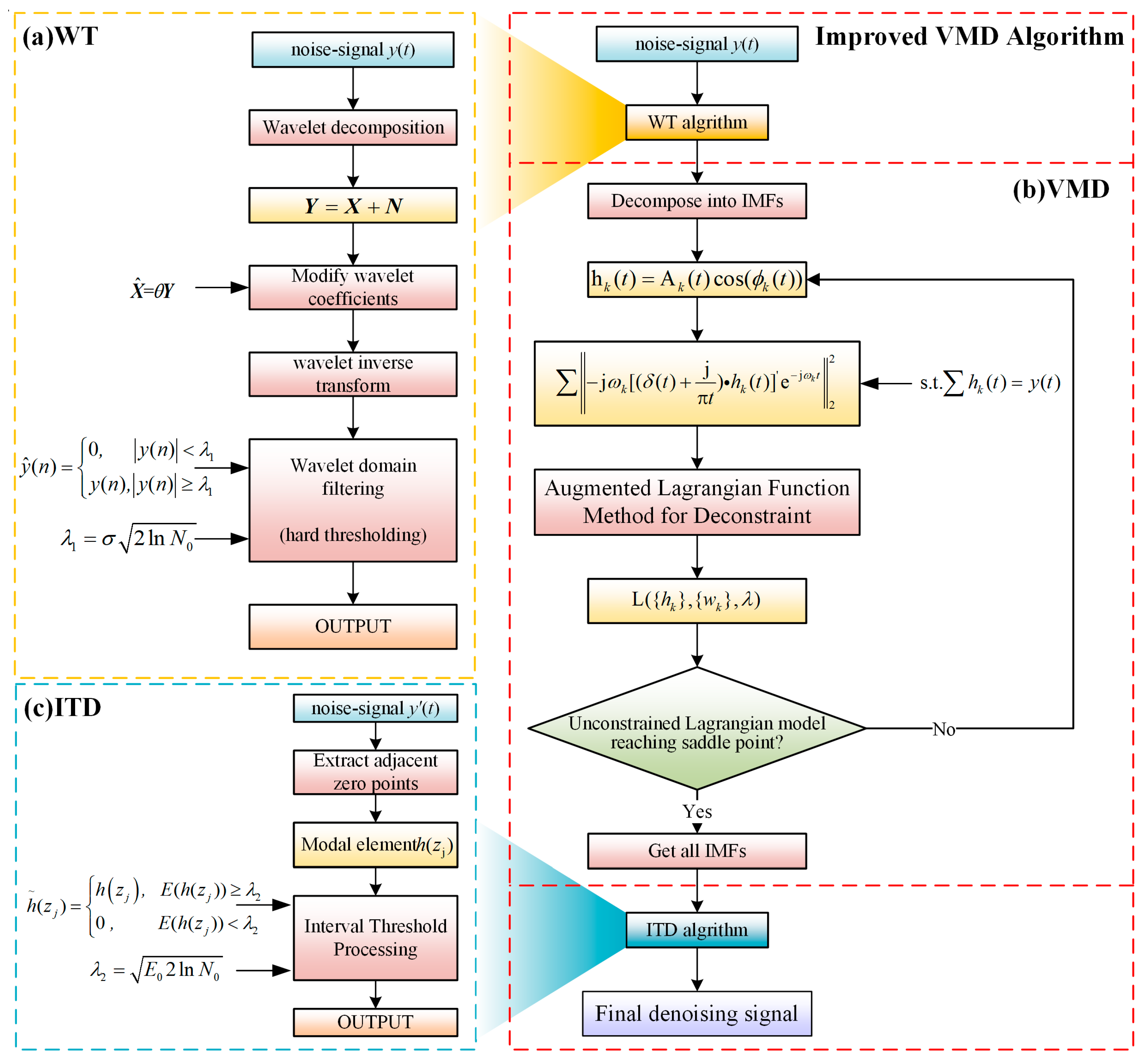
2. Improved VMD-Based Fusion Denoising Algorithm

At present, the existing classical denoising algorithms and some improved algorithms for them often only perform independent denoising processing within different components, ignoring the coupling and superposition between different types of noise, resulting in their sensitivity to one type of noise and low sensitivity to other noises. For example, the traditional VMD [30] algorithm decomposes the original signal into several IMF components by constructing and solving constrained variational problems. When analyzing low signal-to-noise ratio signals containing multiple types of noise, it is prone to severe modal aliasing and end effects. It is difficult to effectively remove the background noise of the signal, significantly affecting the time–frequency analysis results. Therefore, this paper proposes a fusion denoising algorithm based on improved VMD, as shown in Figure 1, including wavelet transform, variational mode decomposition, and interval threshold denoising processing. This paper proposes fusion denoising algorithms that utilize the different sensitivity of denoising methods to noise components from various sources. The aim is to eliminate complex noise and improve the quality of the processed data.

2.1. Wavelet Transform Preprocessing

Wavelet transform is a local transform. It uses a finite-length decaying wavelet base $\psi (t)$ instead of an infinite-length trigonometric function base $e^{i\omega t}$ to achieve localization of time and frequency [16]. Wavelet domain filtering is a method that uses wavelet transform to denoise signals. Its basic idea is based on the characteristics that the wavelet coefficients of noise and signals have different intensity distributions in different frequency bands. The wavelet coefficients with absolute values smaller than the appropriate threshold are set to zero or shrunk, while the wavelet coefficients with larger absolute values are retained. Then, the processed coefficients are reconstructed by wavelet transform to obtain a pure signal.

This paper selects the most commonly used S8 wavelet in symletsN wavelets, whose wavelet base is:

$$\psi (t)=-\frac{1}{8}{t}^3{e}^{-\frac{t}{2}}u(t)+\frac{1}{4}t{e}^{-\frac{t}{2}}u(-t)$$

(1)

where $u(t)$ is the unit function, and $t$ is the time. The formula of wavelet transform is:

$$\mathrm{WT}(a,\tau )=\frac{1}{\sqrt{a}}{\displaystyle {\int }_{-\infty }^{\infty }f(t)}\psi (\frac{t-\tau }{a})dt$$

(2)

where $a$ is the scale, and $\tau$ is the translation. The noisy signal is denoted as $\mathit{y}=\mathit{x}+\mathit{n}$, where $\mathit{x}$ is the original signal, and $\mathit{n}$ is Gaussian white noise with variance ${\sigma }_n^2$. The process, as shown in Figure 1a, is:

Step 1: Wavelet transform is performed on the noisy signal to obtain $\mathit{Y}=\mathit{X}+\mathit{N}$, where $\mathit{Y}$, $\mathit{X}$, and $\mathit{N}$ are, respectively, wavelet transform coefficients of $\mathit{y}$, $\mathit{x}$, and $\mathit{n}$.

Step 2: The wavelet coefficients are modified to obtain an estimate of the wavelet transform coefficients of the noise-free signal.

Step 3: Wavelet inverse transform is performed on the modified wavelet domain coefficients to reconstruct the denoised signal.

The estimated value of $\mathit{X}$ is $\widehat{\mathit{X}}=\theta \mathit{Y}$, where $\theta$ is the filter correction coefficient. However, since the wavelet coefficient ${\theta }_{\mathrm{ideal}}$ is unknown, it is necessary to adjust the design of the filter according to signal characteristics and denoising requirements. A common method is to set a threshold, whereby the wavelet coefficients with amplitudes lower than the threshold are set to zero, and the wavelet coefficients higher than the threshold are either fully retained or subjected to corresponding “shrinkage” processing, which can be expressed in the form of a formula:

$$\widehat{y}(n)=\left\{\begin{array}{l}0,\hspace{1em}\left|y(n)\right|<{\lambda }_1\\ y(n),\left|y(n)\right|\ge {\lambda }_1\end{array}\right.$$

(3)

where $\widehat{y}(n)$ represents the output after threshold filtering, $y(n)$ represents the noisy signal, ${\lambda }_1=\sigma \sqrt{2\ln N_0}$ represents the threshold value, $\sigma$ represents the standard deviation of the signal, and $N_0$ is the length of the signal. After testing, wavelet transform can effectively filter out high-frequency electromagnetic noise but is not sensitive to low-frequency vibration noise and needs further processing.

2.2. Variational Mode Decomposition

The VMD algorithm is a time–frequency analysis method. The goal is to decompose the original signal into a sum of multiple uniform intrinsic mode functions, as shown in Figure 1b. This algorithm defines IMFs as AM-FM (amplitude-modulated frequency-modulated) functions with bandwidth limitations. The function of the VMD algorithm is to construct and solve constrained variational problems to decompose signals into IMF components:

$$h_k(t)=A_k(t)\cos ({\varphi }_k(t))$$

(4)

where $A_k(t)$ is the amplitude envelope of the intrinsic mode function $h_k(t)$, and ${\varphi }_k(t)$ is the instantaneous phase of $h_k(t)$. $A_k(t)$ and the instantaneous angular frequency ${\omega }_k(t)={\varphi }_k{}^{\prime }(t)$ change slowly compared with ${\varphi }_k(t)$.

Given a noisy original signal $y(t)$, find $k$ narrow-bandwidth $h_k(t)$ with each component corresponding to the center frequency ${\omega }_k(t)$, and corresponding constrained variational model [30]:

$$\begin{array}{l}\underset{\left\{h_k\right\},\left\{w_k\right\}}{\min }\left\{\left.{\displaystyle \sum ‖{-j{\omega }_k{[(\delta (t)+\frac{j}{\mathsf{\pi }t})•h_k(t)]}^{\prime }{e}^{-j{\omega }_{k}t}‖}_2^2}\right\}\right.\\ \text{s.t.}{\displaystyle \sum h_k(t)=y(t)}\end{array}$$

(5)

where $\left\{h_k\right\}=\{h_1,h_2\cdots h_k\}$ is a collection of all intrinsic mode functions obtained using VMD decomposition, $\left\{{\omega }_k\right\}=\{{\omega }_1,{\omega }_2\cdots {\omega }_k\}$ is a collection of center angular frequencies for each intrinsic mode function, and $\delta$ is a Dirac distribution. In order to solve this constrained variational problem for an optimal solution, the augmented Lagrange function is first used to convert the above equality constraint optimization problem into an unconstrained optimization problem, as follows:

$$L(\{h_k\},\{w_k\},\lambda ):=\alpha {{\displaystyle \sum _{}‖{\partial }_t[(\delta (t)+\frac{j}{\pi t})\ast h_k(t)]e^{-j{\omega }_{k}t}‖}}_2^2+{‖y(t)-{\displaystyle \sum _{}{h}_k(t)}‖}_2^2+〈\lambda (t),y(t)-{\displaystyle \sum _{}{h}_k(t)}〉$$

(6)

where $\lambda$ is the Lagrange multiplier, which converts the constraint condition into part of the objective function, then uses the multiplier alternating direction algorithm to solve this unconstrained problem and find the optimal solution of the original problem. After VMD decomposition, IMFs are finally obtained, containing signal and noise characteristics of different frequencies. The IMFs containing the primary signal are reconstructed, which can effectively remove low-frequency vibration noise. However, the background noise in the signal IMFs is coupled with metal debris-like sinusoidal pulses and is difficult to separate. This paper will improve the signal reconstruction process of VMD through interval thresholds.

2.3. Interval Threshold Filtering for IMFs of VMD

Since a noisy signal will have many zeros, the waveform between adjacent zeros can be regarded as a modal unit, so each waveform signal is composed of a series of modal units. The interval threshold denoising proposed in this paper takes each modal unit as an object for threshold processing, as shown in Figure 1c. By detecting the signal strength of each modal unit according to a preset power threshold, it retains modal units with an average power exceeding the threshold and sets zero modal units with average power below the threshold:

$$\tilde{h}(z_j)=\left\{\begin{array}{l}h\left(z_j\right),E(h(z_j))\ge {\lambda }_2\\ 0,\hspace{1em}E(h(z_j))<{\lambda }_2\end{array}\right.$$

(7)

where $j=1,2,\cdots N_z$ represents the j-th modal unit, $N_z$ represents the total number of modal units in the signal, $h(z_j)$ represents the instantaneous value of the signal between the zero points $z_j$ and $z_{j+1}$, $\widetilde{h(z_j)}$ represents the output after interval threshold denoising, $E()$ represents the power of the signal, $E_0$ is the average power of this segment of signal, and ${\lambda }_2=\sqrt{E_{0}2\ln N_0}$ represents the threshold.

After this processing, complex noise from multiple sources, such as high-frequency electromagnetic noise, low-frequency vibration noise, and background white noise, are eliminated individually. The waveform of the denoised signal restores the time–frequency characteristics of the original debris signals.

3. Oil Debris Signal Detection Method Based on DSS-LSTM

After the fusion denoising processing, the original characteristics of the oil debris signal waveform can be restored. However, the particle shape will distort the signal characteristics, causing the traditional waveform recognition method based on signal morphology to fail [13]. To address the above problem, this paper proposes a detection method based on DSS-LSTM (LSTM pretreated with DSS), as shown in Figure 2. Firstly, extract the aged engine oil and collect debris signals based on sensors. Secondly, perform the fusion denoising mentioned above. Next, use the deep scattering spectrum algorithm to clearly show the detailed information that cannot be extracted from the original signal under a multi-resolution analysis framework. Then, provide the calibrated debris signal data to the LSTM network for classification training, automatically extract features from the time series scattering spectrum, and obtain accurate classification mapping relationships. Finally, adjust and optimize the neural network hyperparameters through the BO (Bayesian optimization) algorithm to complete LSTM detection model training and deployment.

3.1. Data Mapping Based on Deep Scattering Spectrum

DSS is a signal analysis method that uses multiple filters to extract different levels of features from input data. Unlike DNN (deep neural network), which uses customizable expansion methods to extract information from filters, DSS uses a set of fixed expansion filters with WST (wavelet scattering transform) as its core. In scattering matrix theory, multi-level decomposition is usually used to describe the scattering process. The local invariant features $\mathit{f}$ of each level are generated using the convolution function $S_{0}f(t)=\mathit{f}\ast {\varphi }_J(t)$ and calculated by wavelet transform in the following way [31]:

$$\left|W_1\right|\mathit{f}={\left\{S_{0}f(t),\left|\mathit{f}\ast {\psi }_{j_1}(t)\right|\right\}}_{j_1\in {\wedge }_1}$$

(8)

where $\ast$ represents the convolution operator, ${\varphi }_J(t)$ represents the low-pass filter, $\psi (t)$ represents the wavelet base function, $j$ represents scale, and $\wedge$ represents the wavelet index family. When performing WST processing on $f(t)$, first create the wavelet function $\psi (t)$ and the low-pass filter $\varphi$ covering all frequencies in the signal. By averaging the wavelet coefficients, a first-order scattering coefficient can be calculated as follows:

$$S_{1}f(t)={\left\{\left|\mathit{f}\ast {\mathit{\psi }}_{j_1}\right|\ast {\varphi }_j(t)\right\}}_{j_1\in {\wedge }_1}$$

(9)

where $S_{1}f(t)$ is the low-frequency component of $\left|\mathit{f}\ast {\mathit{\psi }}_{j_1}\right|$, and $\varphi (t)$ represents the low-pass filter. High-frequency components can be extracted in the following way:

$$\left|W_2\right|\left|\mathit{f}\ast {\mathit{\psi }}_{j_1}\right|={\left\{S_{1}f(t),\left|\left|\mathit{f}\ast {\mathit{\psi }}_{j_1}\right|\ast {\mathit{\psi }}_{j_2}(t)\right|\right\}}_{j_2\in {\wedge }_2}$$

(10)

The calculation process of second-order scattering coefficients is as follows:

$$S_{2}f(t)={\left\{\left|\left|\mathit{f}\ast {\mathit{\psi }}_{j_1}\right|\ast {\mathit{\psi }}_{j_2}\right|\ast {\varphi }_j(t)\right\}}_{j_i\in {\wedge }_i},i=1,2$$

(11)

By iterating the above process, get wavelet modulus convolution:

$$U_{n}f(t)={\left\{\left|\left|\left|\mathit{f}\ast {\mathit{\psi }}_{j_1}\right|\ast \cdots \cdots \left|\ast {\mathit{\psi }}_{j_n}\right.\right|\right.\right\}}_{j_i\in {\wedge }_i},i=1,2,\dots ,n.$$

(12)

By averaging all wavelet modulus convolution coefficients $\left(U_{n}f(t)\right)$ obtain n-order scattering coefficients:

$$S_{n}f(t)={\left\{\left|\left|\left|\mathit{f}\ast {\mathit{\psi }}_{j_1}\right|\ast \cdots \cdots \left|\ast {\mathit{\psi }}_{j_n}\right.\right|\ast {\varphi }_j(t)\right.\right\}}_{j_i\in {\wedge }_i},i=1,2,\dots ,n.$$

(13)

The final scattering matrix can be represented in the following way:

$$Sf(t)={\left\{S_{n}f(t)\right\}}_{0\le n\le l}$$

(14)

where $l$ represents the maximum decomposition order. Splicing all feature vectors collected at all decomposition levels can obtain a scattering matrix for the entire scattering process. Then, these feature vectors composed of scattering matrices will be used to train and recognize deep learning networks.

3.2. Metal Debris Signal Recognition Model Based on LSTM

LSTM is a particular type of RNN (recurrent neural network), which can transform lower-level features into higher-level features through nonlinear transformation, and follows more profound rules [32]. The input data of the LSTM network used in this paper comprise cell state $C_{t-1}$ passed from the previous time series, output information $h_{t-1}$, and current input $x_t$. The output data are cell state $C_t$ and output information $h_t$ at the current time. $C$ and $h$ are also called long-term and short-term memory. The gated unit includes input gate $f_t$, forget gate $i_t$, and output gate $o_t$. Their definitions are as follows [32]:

$$f_t=\sigma \left({\mathit{w}}_f\cdot \left[h_{t-1},x_t\right]+b_f\right)$$

(15)

$$i_t=\sigma \left({\mathit{w}}_i\cdot \left[h_{t-1},x_t\right]+b_i\right)$$

(16)

$$o_t=\sigma \left({\mathit{w}}_o\cdot \left[h_{t-1},x_t\right]+b_o\right)$$

(17)

where $\mathit{w}$ is the reset gate weight, $b$ is the bias term, and the activation function is as follows:

$$\sigma (x)=\frac{1}{1+e^{-x}}$$

(18)

$$\tanh (x)=\frac{e^x-e^{-x}}{e^x+e^{-x}}$$

(19)

The output results of long-term memory $C_t$ and short-term memory $h_t$ are:

$$C_t=f_t\otimes C_{t-1}\oplus i_t\otimes \left(\tanh ({\mathit{w}}_c\cdot \left[h_{t-1},x_t\right]+b_c)\right)$$

(20)

$$h_t=o_t\otimes \tanh (C_t)$$

(21)

where $\otimes$ is element multiplication, and $\oplus$ is element addition. Considering the time series characteristics of oil debris signals processed using DSS, this paper constructs an overall LSTM debris detection recurrent neural network architecture, as shown in Figure 3. Here, time series sample $X_i=(x_1,x_2,\cdots ,x_i,\cdots x_S)$, $x_i$ represents multi-channel spectral data corresponding to sampling point $i$ after DSS processing, and subscript $S$ is the total length after time series processed using DSS.

Firstly, a segment sample sequence ${\mathit{X}}_i$ placed at the input layer is input into the LSTM module in the hidden layer to drive an update of cell state $C$ and output $h$. After feature extraction and transmission through the neural network hidden layer, the signal is output to the output layer through the last LSTM module. In the output layer, the signal passes through a fully connected layer, a SoftMax layer, and a classification output layer successively to obtain the normalized probability ${\mathit{Y}}_i{}^{\prime }=(y_1{}^{\prime },y_2{}^{\prime },\cdots y_C{}^{\prime })$ of the LSTM network’s prediction category of the signal, and the result is input into correction layer for further step processing. Then the loss function is defined, which measures the degree of discrepancy between the model’s predictions and the actual values:

$$Loss=-{\displaystyle \sum _{i=1}^C{p}_i}\log y_i{}^{\prime }$$

(22)

where $y_1{}^{\prime },y_2{}^{\prime },\cdots y_C{}^{\prime }$ represents the normalized probability of different categories, $C$ is the total number of signal categories ($C=3$ in this paper), and $p_i$ is the actual probability of the signal category obtained from the ${\mathit{X}}_i$ corresponding label. If a signal category is in the $i-th$ class, then $p_i=1$, otherwise $p_i=0$; in the correction layer, according to $Loss$, the matrix $\mathit{w}$ is updated based on gradient optimization to complete the LSTM algorithm update.

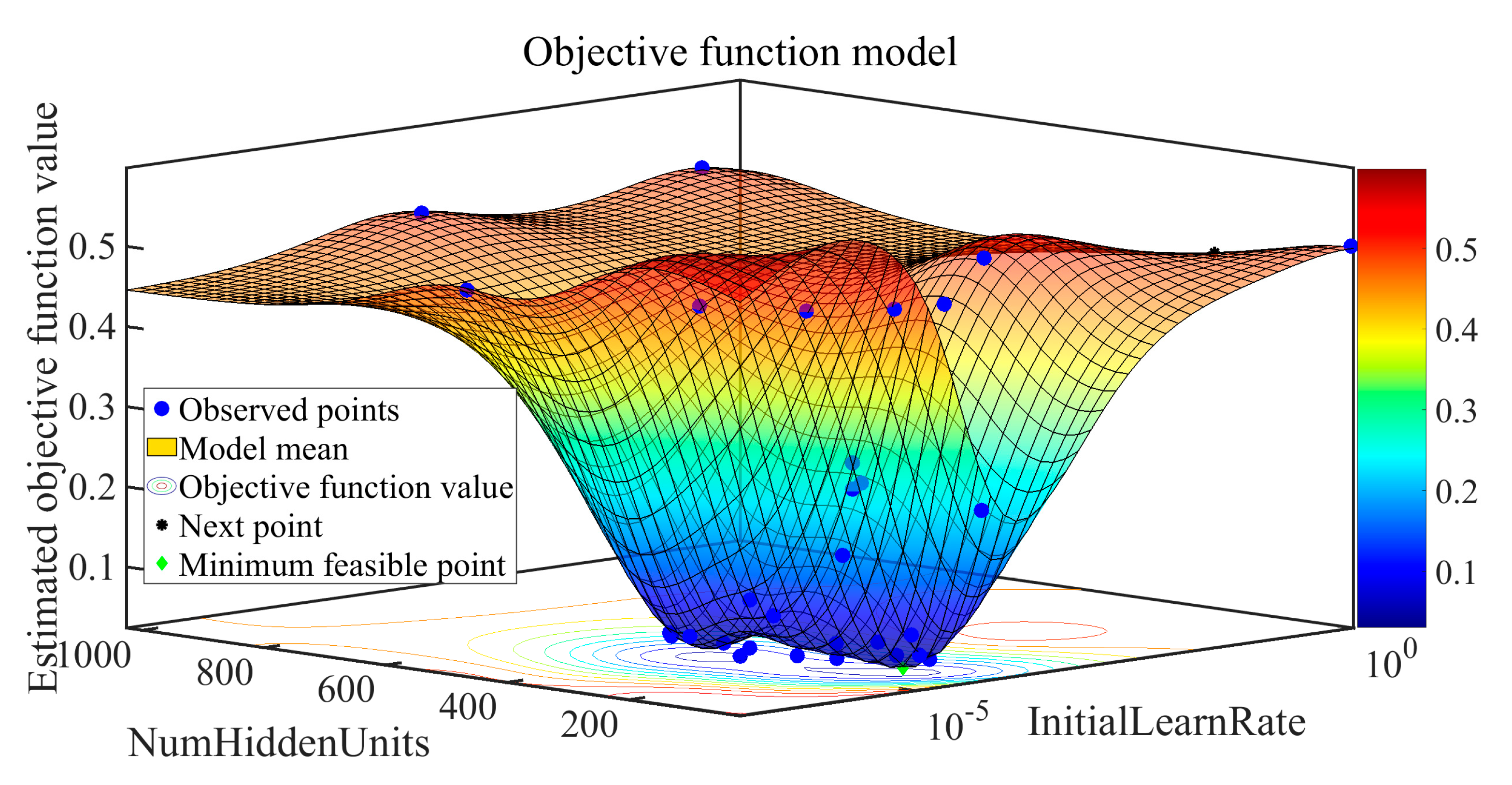
3.3. Hyperparameter Optimization Based on Bayesian Optimization

Neural network hyperparameters are among the most critical factors determining network classification accuracy. The Bayesian optimization algorithm quickly searches for the optimal target value through finite iterations under a prior probability distribution [33] suitable for hyperparameter optimization in deep learning networks. This paper defines the hyperparameter group as a variable value and the difference between classification accuracy and loss value as the objective function. Specific definitions and relationships are as follows [34]:

$$f^{\prime }(\mathit{a})=A\times 100-\mathrm{abs}(Loss)(\mathit{a}=a_1,a_2,\dots ,a_n)$$

(23)

$${\mathit{a}}^{\ast }=\mathrm{argmax}{f}^{\prime }(\mathit{a})$$

(24)

where $\mathit{a}$ represents the hyperparameter group $a_1,a_2,\dots ,a_n$, $f^{\prime }(\mathit{a})$ represents the target value corresponding to variable $\mathit{a}$, $A$ is the classification accuracy value of the network with hyperparameters $\mathit{a}$ proposed, $Loss$ is obtained using Equation (22), $\mathrm{abs}(.)$ is used to obtain the absolute value of the input data, $\mathrm{argmax}$ represents the maximum value of the objective function, and ${\mathit{a}}^{\ast }$ is the optimal variable value predicted based on the Bayesian principle as follows:

$$p(f^{\prime }|{\mathit{D}}_{1:t})=\frac{p({\mathit{D}}_{1:t}|f^{\prime })p(f^{\prime })}{p({\mathit{D}}_{1:t})}$$

(25)

where ${\mathit{D}}_{1:t}=\left\{\left({\mathit{a}}_1,f^{\prime }({\mathit{a}}_1)\right),\left({\mathit{a}}_2,f^{\prime }({\mathit{a}}_2)\right),\dots ,\left({\mathit{a}}_t,f^{\prime }({\mathit{a}}_t)\right)\right\}$ is the collection of observation samples, $f^{\prime }$ is the unknown target function to be optimized, $p(f^{\prime })$ and $p({\mathit{D}}_{1:t}|f^{\prime })$ are prior probability distributions of $f^{\prime }$ and ${\mathit{D}}_{1:t}$, $p({\mathit{D}}_{1:t}|f^{\prime })$ is the probability containing the target value $f^{\prime }$ in ${\mathit{D}}_{1:t}$, and $p(f^{\prime }|{\mathit{D}}_{1:t})$ is the posterior probability distribution of $f^{\prime }$.

Then, the acquisition function is constructed with improvement probability $PI$ to obtain the extreme point of the target function $f^{\prime }$ as the following variable group to improve the current maximum target function.

$$PI(t)=\varnothing (\frac{\mu (t)-f^{\prime }({\mathit{a}}^{\ast })-\epsilon }{\sigma (t)})$$

(26)

where $\mu (t)$ and $\mu (t)$ are the expected value and variance of the posterior probability model, $f^{\prime }({\mathit{a}}^{\ast })$ is the current maximum target value, $\epsilon$ is an adjustable parameter, and $\varnothing (t)$ is the cumulative distribution function of a standard normal distribution. Therefore, the extreme points of the target function $f^{\prime }$ and the target value can be obtained according to the acquisition function.

4. High-Confidence Measurement Method for Oil Debris

Considering the problems of false and missed detections in the measurement process of oil debris and the online output requirements of debris information, this paper proposes a high-confidence measurement method for oil debris, as shown in Figure 4. Firstly, the continuous signal of the oil debris sensor is stored and preprocessed; secondly, the time series is continuously monitored through the improved sliding window scheme while reducing the amount of data processing; then, through the fusion judgment of multi-window information, the confidence of the measurement process is improved, and the false alarm rate and missed detection rate are reduced; finally, based on the electromagnetic measurement principle, information such as debris size is calculated from signal waveform characteristics and output.

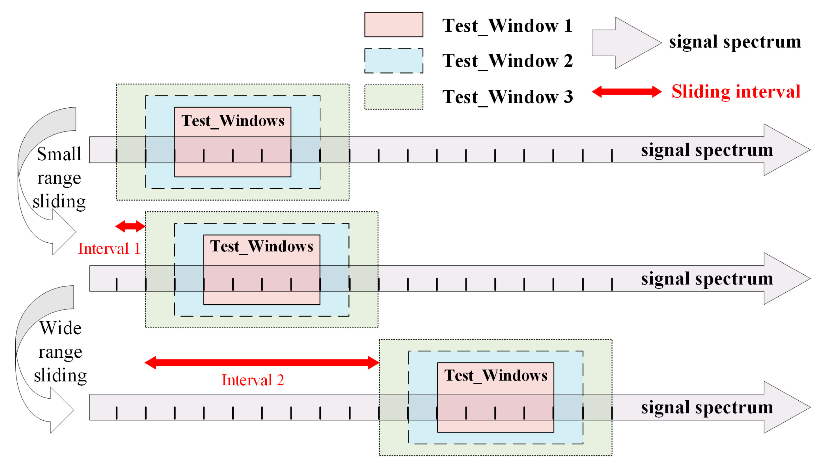
4.1. Detection Method of Multi-Window Information Fusion

To detect a real-time updating waveform signal sequence a windowing operation [35] is necessary. Using a fixed-length window may cause the waveform characteristics of the debris signal to be segmented or mixed, which can affect the classification effectiveness of the detection model and result in missed or false detections. In order to improve the confidence of debris signal detection, this paper proposes a method of multi-length data windowing, as shown in Figure 5. Three different test windows of 200, 300, and 400 are used to extract the waveform signals. The signal sequences of the three windows are fed into the waveform recognition model for detection, and the sliding distance of the window is determined according to the results. A smaller sliding distance (Interval 1 = 50) can improve the accuracy, while a larger distance (Interval 2 = 400) can improve the detection speed and avoid duplicate detections.

The specific sliding debris multi-window fusion detection process, shown in Figure 4, is:

Step 1: The signal of the lubrication system is collected, stored, segmented, and denoised.

Step 2: The starting point and length of the window are determined, and it is judged whether to splice new signal data based on the remaining length of the time series.

Step 3: The signals of the three windows are subjected to DSS preprocessing and LSTM model classification, and the debris detection results with confidence above the threshold are retained.

Step 4: It is determined whether there are two or more debris signals of the same type in the retained results. If not, it is considered a false detection, and the window starting point is determined by sliding with Interval 1; if so, the type, number, location, and amplitude of the debris are recorded, and the size information of the debris is calculated based on the electromagnetic measurement principle.

Step 5: Relevant information is outputted, and the sliding window continues with Interval 2 until the measurement is completed.

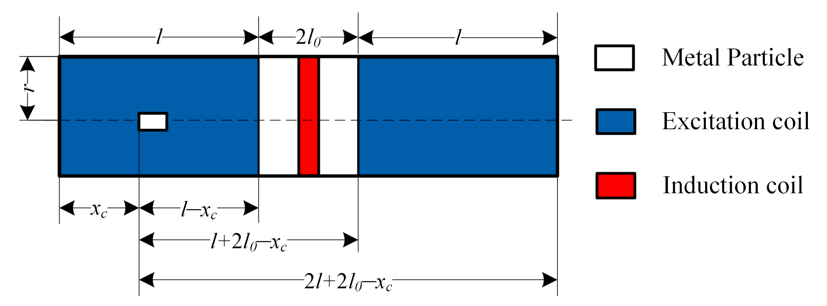
4.2. Principle of Electromagnetic Metal Debris Sensor

The internal structure principle model of the electromagnetic oil debris sensor is shown in Figure 6. The blue areas on both sides represent symmetrical excitation coils, and the red area in the middle represents the secondary induction coil. The number of coil turns is 1, located in the center of two excitation coils. Metal debris enters the sensor at $x_c$ with velocity $v_0$, radius $r_c$ and length $l_c$. It is assumed that it is ferromagnetic and has the relative magnetic permeability ${\mu }_c$ and that its shape is cylindrical with volume $V_c$ just at the solenoid axis.

Based on Lenz’s law and the electromagnetic induction law, the induced electromotive force amplitude $E_{1\max }$ of ferromagnetic debris is calculated [36]:

$$E_{1\max }=-\frac{M{U}_s}{L_0{}^2}{N}_c\frac{{\mu }_0{\mu }_c{N}_c}{2l^2}{V}_c\left[\frac{x_c}{\sqrt{r^2+x_c{}^2}}+\frac{l-x_c}{\sqrt{r^2+{\left(l-x_c\right)}^2}}\right]\sqrt{1+{(\frac{v_0{r}^2}{\omega }R)}^2}$$

(27)

where $M$ is the mutual inductance between the two excitation coils and the induction coil, ${\mu }_0$ is the vacuum magnetic permeability $U_s$ is the amplitude of the excitation coil’s voltage, $N_c$ is the turn number of the measurement coil, $R$ is a characteristic parameter of debris only related to a sensor’s structure size and position and the velocity of metal debris, and the expression of $R$ is:

$$\begin{array}{ll}R=& \frac{v_0{r}^2\sqrt{r^2+{\left(l-x_c\right)}^2}}{\omega \left(r^2+x_c{}^2\right)\left(x_c\sqrt{r^2+{\left(l-x_c\right)}^2}+\left(l-x_c\right)\sqrt{r^2+x_c{}^2}\right)}\hfill \\ & -\frac{v_0{r}^2\sqrt{r^2+x^2}}{\omega \left(r^2+{\left(l-x_c\right)}^2\right)\left(x_c\sqrt{r^2+{\left(l-x_c\right)}^2}+\left(l-x_c\right)\sqrt{r^2+x_c{}^2}\right)}\hfill \end{array}$$

(28)

If metal particles are non-ferromagnetic materials they can be regarded as short-circuit coils connected with an excitation coil magnetically. The alternating current flowing in an excitation coil will generate an alternating magnetic field in space, which will induce an internal current in the metal particles. Its internal current is excited by excitation coil 1 to cause induction electromotive force $E_{2\max }$ in the induction coil [36]:

$$E_{2\max }=r_c{}^4{A}_s\sqrt{{(K\omega )}^2+{(\frac{dK}{dt})}^2}$$

(29)

where $A_s$ is the amplitude of the excitation coil’s current, $\omega$ is the angular frequency of the excitation coil’s current, and $K$ is the characteristic parameter of non-ferromagnetic debris only related to a sensor’s structure size and position and the shape of metal debris:

$$K=\frac{{\mu }_0{\pi }^{3}NG{r}^2}{2l_c\left(\ln \frac{2l_c}{r_c}-0.75\right)l{(l+l_0-x_c)}^3}$$

(30)

According to Equation (27), when ferromagnetic metal debris appears inside the sensor at the same speed, the waveform amplitude $E_{1\max }$ of the metal debris signal is only related to volume $V_c$ of the debris and can be approximated as being proportional to the cube of radius $r_{c1}$:

$$E_{1\max }/E_{1\max }{}^{\prime }={(r_{c1}/r_{c1}{}^{\prime })}^3$$

(31)

where $E_{1\max }{}^{\prime }$ and $r_{c1}{}^{\prime }$ represent the calibrated signal amplitude and radius of ferromagnetic metal debris, respectively.

When non-ferromagnetic metal debris appears inside the sensor at the same speed, the waveform amplitude $E_{2\max }$ of the metal debris signal can be approximated as being proportional to the fourth power of radius $r_{c2}$ according to Equation (29), that is:

$$E_{2\max }/E_{2\max }{}^{\prime }={(r_{c2}/r_{c2}{}^{\prime })}^4$$

(32)

where $E_{2\max }{}^{\prime }$ and $r_{c2}{}^{\prime }$ represent the calibrated signal amplitude and radius of non-ferromagnetic metal debris, respectively.

5. Simulation and Experimental Verification

In order to verify the effectiveness of the fusion denoising algorithm proposed in this paper and provide a detection model for debris measurement in oil systems, in this part we first conduct a denoising test and waveform recognition test based on debris sensor data, then carry out training and optimization of a debris signal recognition network, and finally carry out measurement experiments.

5.1. Oil Debris Signal Denoising Simulation Experiment

5.1.1. Comparison of Traditional Denoising Methods

This paper selects four typical denoising schemes from the current literature for comparative testing. Scheme 1 (WT) [16]: WT filtering processing of the original signal; Scheme 2 (VMD) [30]: VMD processing of the original signal and removal of the noise mode; Scheme 3 (WT-VMD) [37]: WT filtering processing of the original signal first, then VMD processing of the filtered signal; Scheme 4 (VMD-WT) [38]: VMD processing of the original signal first and removal of the noise mode, then WT filtering processing of the denoised signal.

Firstly, the background noise (SNR ≈ −5.5 dB) (signal-to-noise ratio) of the oil system is superimposed with Gaussian white noise to simulate different intensity noise backgrounds (SNR ≈ −5.5 dB~−11.5 dB). Then, the ideal debris signal waveform is added as a test signal into background noise to obtain the original signal. Finally, four denoising methods are used to process it to obtain the denoised signal. In different intensity noise backgrounds, 1000 Monte Carlo experiments were carried out. The SNR, XCORR (cross-correlation coefficient), and MSE (mean squared error) results after denoising are shown in Figure 7:

As can be seen from Figure 7, under a typical background noise intensity of −5.5 dB~−11.5 dB, the signal processed using the Scheme 3 (WTD-VMD) algorithm has the highest SNR (greater than 6 dB), highest XCORR (greater than 0.85), and lowest MSE (less than 10⁻⁴) indicating that different denoising algorithms can effectively suppress noise intensity after combination and retain instantaneous amplitude and time–frequency information of the original signal. In addition, the results of Scheme 2 (VMD) and Scheme 4 (VMD-WT) in Figure 7 are very close, indicating that algorithms cannot be combined arbitrarily when designing a denoising combination. An appropriate order needs to be designed according to the characteristics of the algorithm.

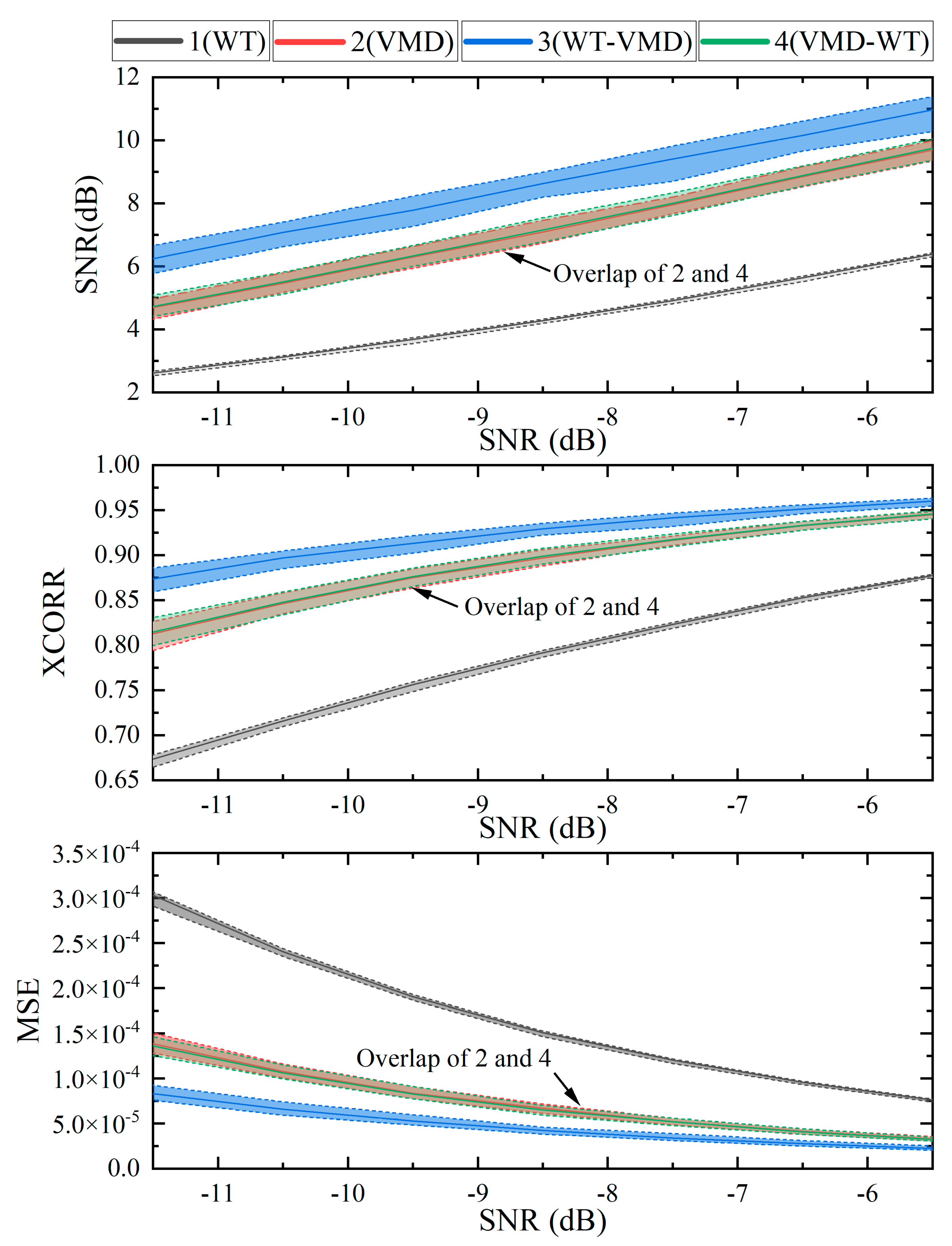
5.1.2. Test of the Improved VMD Fusion Denoising Algorithm

Based on the above experiment, in this part we conduct a comparative test between the WT-VMD method [37] with the best effect and the improved VMD fusion denoising algorithm proposed in this paper. The results are shown in Figure 8. Compared with the WTD-VMD method, the SNR of this paper’s algorithm is increased by about 4 dB after denoising, the XCORR is increased by about 0.08, and the MSE is reduced by about four times.

Figure 9 shows a set of debris signals after denoising processing. It can be seen that after processing using the improved VMD fusion denoising algorithm, complex noise from multiple sources, such as high-frequency noise, low-frequency vibration noise, and white noise, is effectively eliminated. Compared with the WT-VMD method, the signal after denoising using this paper’s algorithm reduces low-power sine-like low-frequency waveform interference. It is closer to an ideal sine–cosine waveform of metal debris. It can effectively extract metal-like sine signals from oil debris under a complex environment.

5.2. Oil Debris Signal Denoising Simulation Experiment

5.2.1. DSS-LSTM Training Process Based on BO

For this paper we select denoised debris sensor data for data calibration. We select signal sequences of different flow rates and different particle sizes, totaling 8089 groups, including 2310 groups of no debris (None), 3469 groups of ferromagnetic debris (Fe), and 2310 groups of non-ferromagnetic debris signals (NFe). After random cropping for data enhancement, DSS scattering preprocessing is performed. Then, the training set and test set are divided according to a ratio of 8:2. Then, batch size (batch) is set to 128, the total number of iterations to 10,000 rounds, the learning rate decay strategy to exponential decay, the initial learning rate range to 10⁻⁷~1, and LSTM neural network training hyperparameter optimization is carried out based on Bayesian optimization. The target function model estimated using the Bayesian algorithm is shown in Figure 10. The change in the actual optimal value and estimated optimal value of the target function during the optimization process is shown in Figure 11.

The best feasible point observed during the Bayesian optimization process is an initial learning rate of 2.4044 × 10⁻⁵, whereby the number of hidden layers is 359. The best feasible point estimated using the target function model is an initial learning rate is 4.1328 × 10⁻⁵, whereby the number of hidden layers is 136. After verification, choosing the estimated best feasible point for LSTM network training can obtain the best model for oil debris signal recognition.

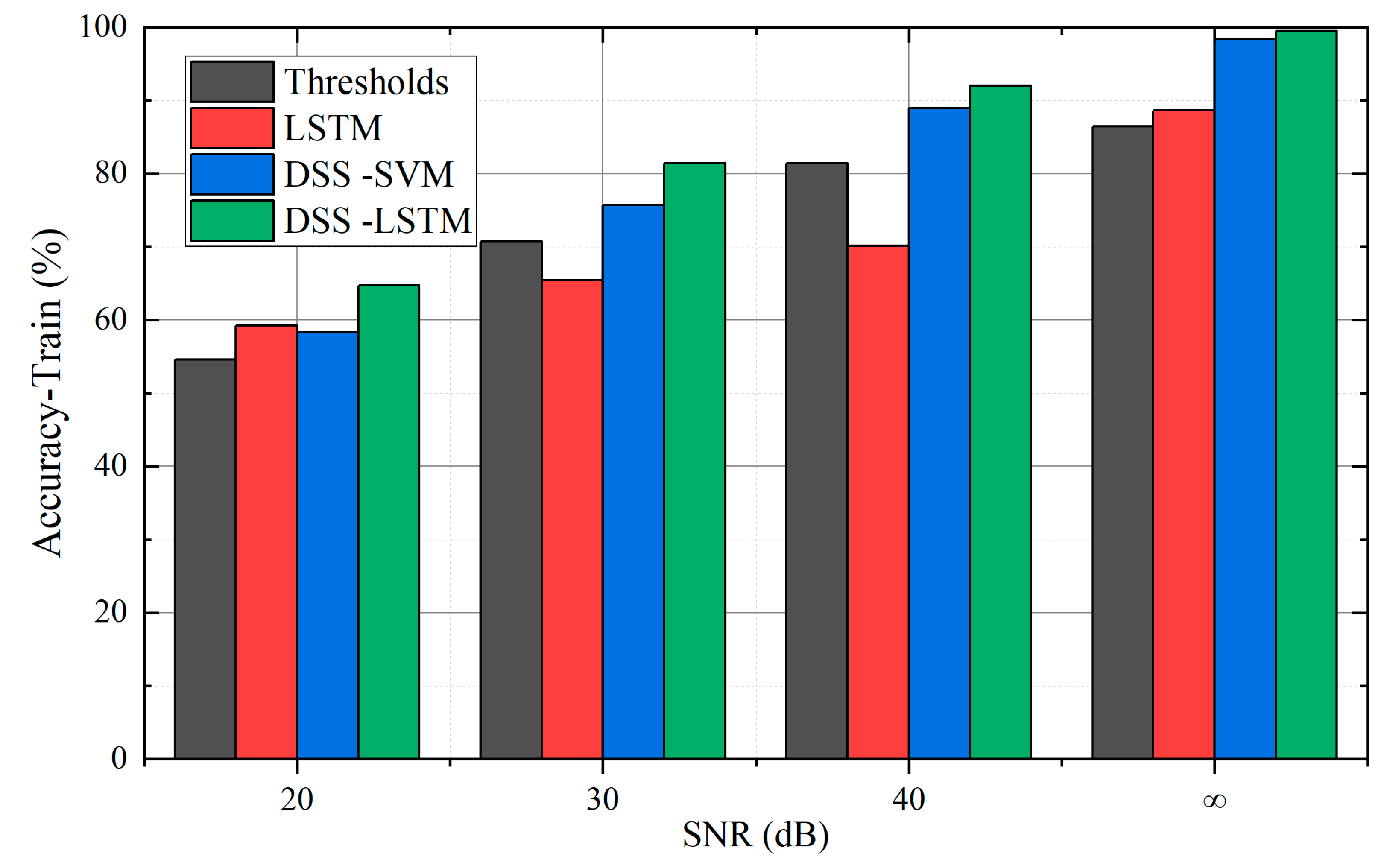
5.2.2. Comparison of Effects of Debris Classification Models

This section compares the effectiveness of different methods for oil debris classification detection. When selecting the comparison object of the selection algorithm, the traditional debris detection method based on threshold judgment [1] is first introduced. Then, referring to the current research [33,39], this paper chooses the LSTM method suitable for a time series and the SVM method suitable for classification for comparison. In addition, a control group with or without DSS preprocessing is set to prove the effectiveness of DSS preprocessing. On this basis, this paper introduces Gaussian white noise with zero means to process original data with different degrees of noise, obtains data under signal-to-noise ratios of 20, 30, 40, and ∞ (no noise added), and verifies the testing effect of different algorithms under noise interference. Finally, the BO algorithm is used to optimize the thresholds and hyperparameters to obtain the optimal testing results of each method. The results are compared as shown in

Table 2. Comparison of debris signal classification models.

SNR	Type	Accuracy (%)				Recall (%)
		All	None	Fe	NFe	All	None	Fe	NFe
20	Thresholds	54.62	39.0	92.9	44.0	54.65	96.7	62.7	0.5
	LSTM	59.21	44.0	95.2	40.7	59.28	68.2	71.7	31.7
	DSS-SVM	58.34	46.0	90.0	37.2	58.34	53.9	72.3	41.8
	DSS-LSTM	64.71	53.4	90.5	44.1	64.72	48.9	82.6	53.7
30	Thresholds	70.76	52.9	96.7	58.0	70.75	88.0	88.4	27.0
	LSTM	65.45	62.3	95.7	44.6	66.04	22.9	83.2	83.4
	DSS-SVM	75.71	66.5	96.8	59.2	76.29	77.7	87.8	57.6
	DSS-LSTM	81.46	65.3	96.6	81.8	81.49	93.1	97.6	45.7
40	Thresholds	81.44	67.7	97.3	77.1	81.48	94.2	90.5	55.2
	LSTM	70.15	49.6	100	73.0	70.89	100	89.6	13.7
	DSS-SVM	89.00	83.0	98.1	84.4	89.65	91.1	95.5	79.4
	DSS-LSTM	92.03	89.6	97.9	85.7	92.03	87.9	98.4	86.6
∞	Thresholds	86.49	87.4	93.3	76.4	86.49	82.6	91.4	83.0
	LSTM	88.63	79.4	100	85.6	88.65	90.4	81.2	98.1
	DSS-SVM	98.44	99.6	99.7	96.4	98.70	96.8	99.7	99.1
	DSS-LSTM	99.51	100	98.9	100	99.51	100	100	98.3

and Figure 12.

Figure 12 and Table 2 show that traditional thresholds methods have low accuracy in different noise backgrounds, making it hard to meet the accuracy requirements of debris measurement. Under no-noise conditions, the accuracy of the DSS-LSTM can reach more than 99.5%, and the accuracy and recall rate of None, Fe, and NFe are all greater than 98%. The accuracy of the DSS-LSTM model meets the application requirements. Under noisy conditions, compared with the LSTM without DSS preprocessing, the performance of the DSS-LSTM improved dramatically, indicating that DSS preprocessing is effective. In addition, in comparison with the DSS-SVM method, the DSS-LSTM method has the highest accuracy under different noises, indicating that the LSTM network is a more suitable method for debris signal classification. The above data show that since non-ferromagnetic signals are weak and quickly submerged by noise, the recognition effect of all methods significantly decreases when noise is enhanced. The results also prove the necessity of researching fusion denoising methods in this paper.

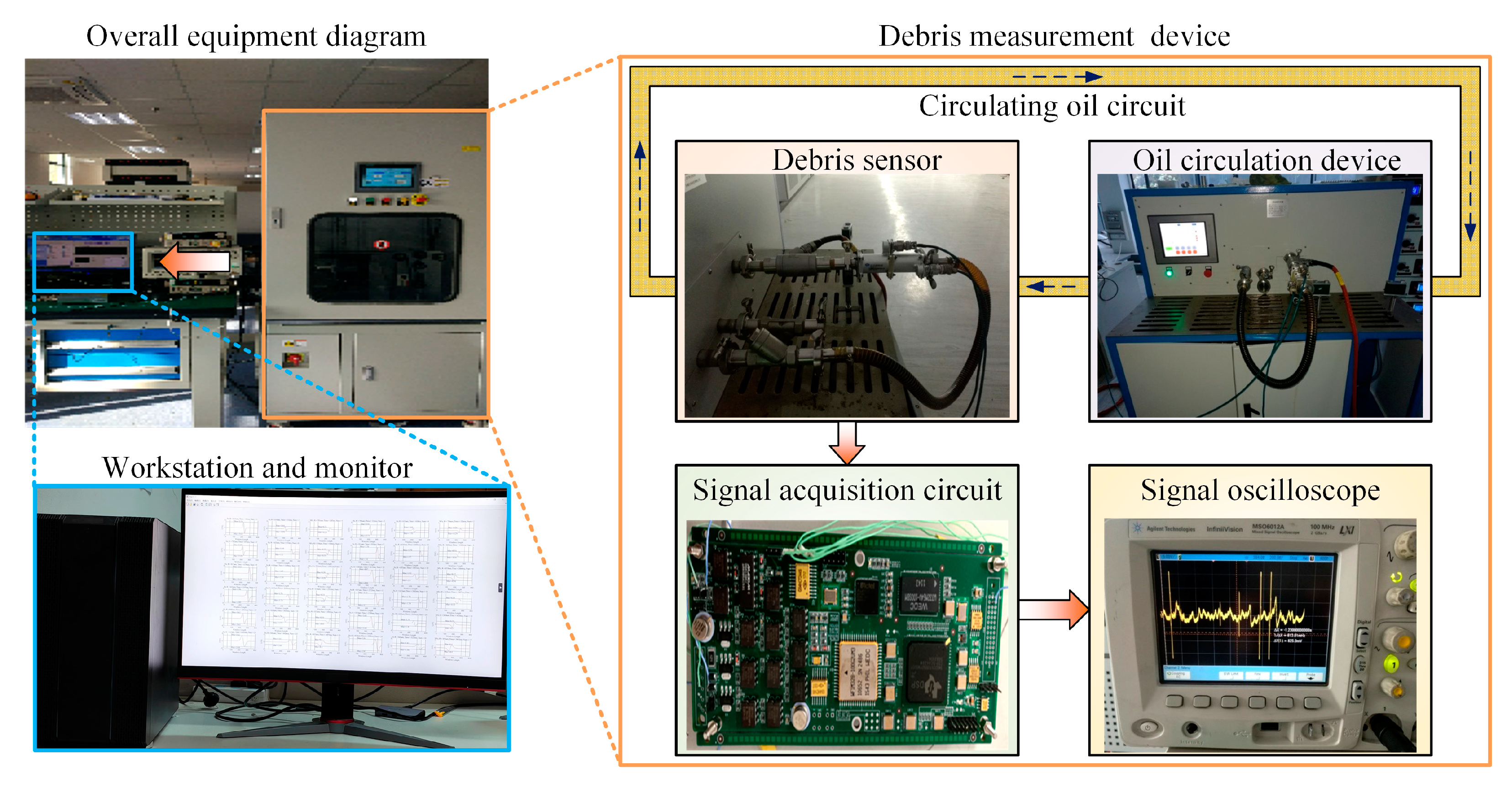
5.3. Oil Debris Signal Measurement Experiment

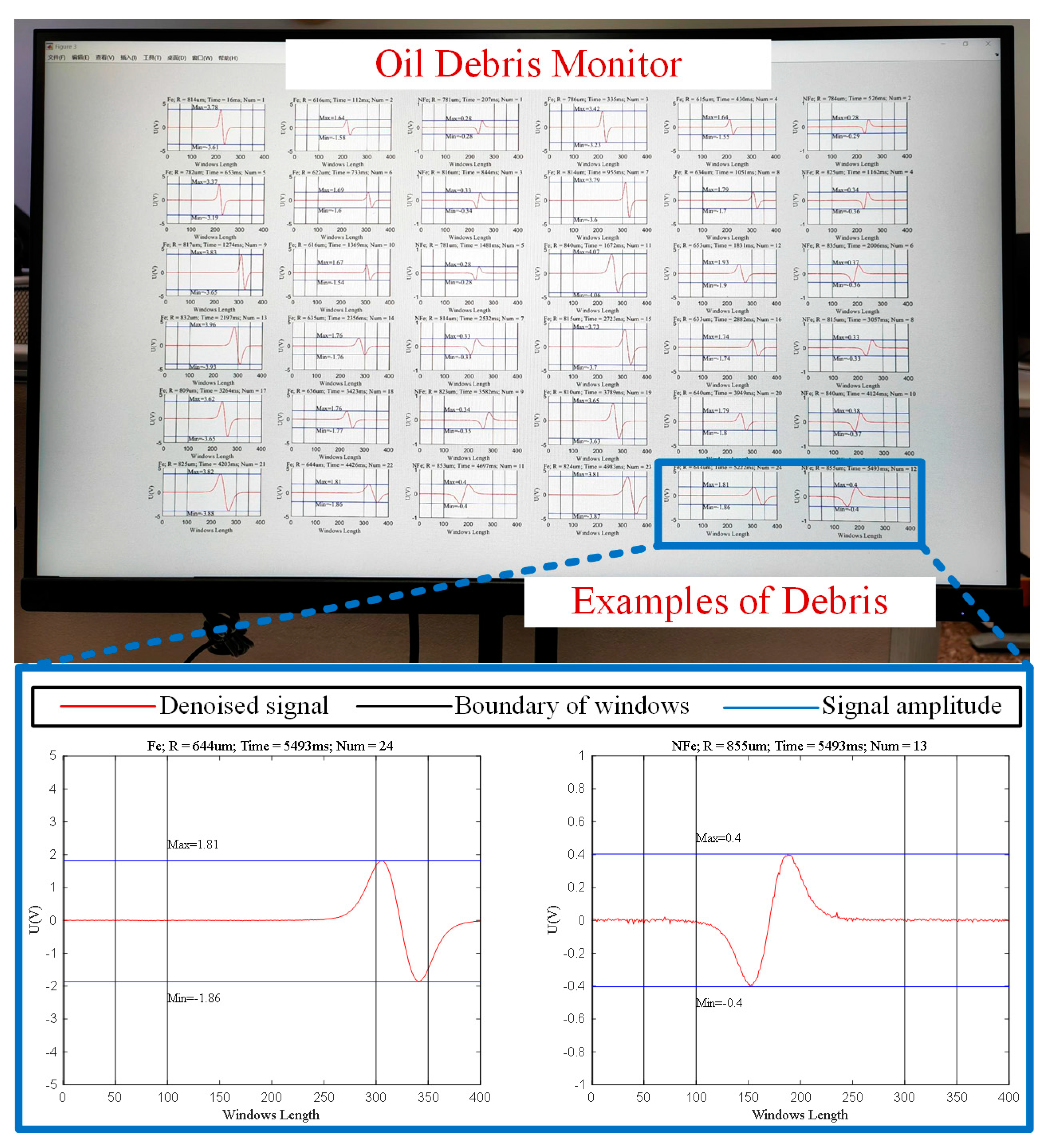
5.3.1. Signal Amplitude Calibration Experiment

In order to provide a reference value for the calculation of debris size for this paper, we conducted an oil circulation experiment for debris amplitude calibration. The experimental equipment shown in Figure 13 is composed of a debris measurement device, a workstation, and a monitor. The debris measurement device consists of a circulating oil circuit, an oil circulation device, a debris sensor, a signal acquisition circuit, and a signal oscilloscope. The experimental process is as follows: First, metal debris particles of different sizes are moved in the circulating oil circuit- Next, debris sensors and signal acquisition circuits are used to collect signals. Then, the oil signal is output to the oscilloscope for display. Finally, the data are stored, calibrated, and processed in the workstation. The collected signal amplitude data are shown in

Table 3. Calibration results for ferromagnetic debris of different sizes.

	Metal Filing Particle Diameter (Fe)
	400 μm		600 μm		800 μm
Speed (m/s)	Peak (V)	Trough (V)	Peak (V)	Trough (V)	Peak (V)	Trough (V)
1	0.6483	−0.6798	1.8959	−1.9917	4.0680	−4.2729
2	0.6315	−0.6455	1.8663	−1.9050	3.9286	−3.9925
3	0.6251	−0.6232	1.8175	−1.8136	3.8367	−3.8300
5	0.5790	−0.5484	1.6988	−1.6057	3.5926	−3.4168

and

Table 4. Calibration results for non-ferromagnetic debris of different sizes.

	Metal Filing Particle Diameter (Fe)
	600 μm		800 μm
Speed (m/s)	Peak (V)	Trough (V)	Peak (V)	Trough (V)
1	1.8959	−1.9917	4.0680	−4.2729
2	1.8663	−1.9050	3.9286	−3.9925
3	1.8175	−1.8136	3.8367	−3.8300
5	1.6988	−1.6057	3.5926	−3.4168

.

5.3.2. Measurement Method Test

For this paper we conducted measurement experiments for oil debris signals under different conditions, such as oil circulation flow rates, particle types, and particle sizes. The oil debris information monitor is shown in Figure 14. The final output information includes the type of debris, particle diameter, position of signal time where debris is located, and the total number of measured particles.

Then, a comparative test was carried out between the traditional sliding window method and the measurement method proposed in this paper. The results are shown in

Table 5. Comparison between multi-window fusion and single-window.

	Accuracy (%)	Error Rate (%)	FAR (%)	Loss (%)	Fe		NFe
					Accuracy (%)	Recall (%)	Accuracy (%)	Recall (%)
Multi-windows	99.76	0.24	0.035	0.24	99.74	100	99.78	99.48
Single-window	93.45	6.55	5.77	0.83	90.46	99.80	98.40	98.23

. Compared with traditional single-window sliding measurements [35], the accuracy of the multi-windows used in this paper increased from 93.45% to 99.76%, higher than the accuracy rate of the LSTM training process of 99.51%; the single accuracy rate and recall rate of Fe and NFe all significantly increased to more than 99% compared with traditional methods; in addition, the error rate of this method dropped from 6.55% to 0.24%, the false alarm rate dropped from 5.77% to 0.035%, and the missed detection rate (loss) dropped from 0.83% to 0.24%, effectively reducing the occurrence of erroneous information during the metal debris recognition process, proving the effectiveness and superiority of the multi-window fusion algorithm.

6. Conclusions

This paper presents a new method for the electromagnetic measurement of metal debris in aero-engine oil systems. The method consists of an improved VMD denoising algorithm, a DSS-LSTM waveform recognition method, and a multi-window fusion detection method, providing new ideas for the problem of low accuracy caused by noise interference and weak signals of electromagnetic debris sensors. This paper demonstrates that it is very necessary to apply targeted noise reduction for different sources of noise in a strong noise background, which can greatly improve the noise reduction level. Moreover, in signal waveform feature recognition, the intelligent algorithm designed based on a neural network has great advantages over the traditional method based on threshold judgment. The main contributions of this paper are as follows:

Firstly, it summarizes previous research experience, uses the differences in sensitivity to different noise of various denoising methods, designs an improved VMD fusion denoising algorithm, and eliminates electromagnetic noise, vibration noise, and background white noise step by step. Secondly, it uses the DSS-LSTM classification network and Bayesian optimization of hyperparameters is carried out to extract and recognize debris characteristics automatically. Then, it improves the confidence of debris measurement through multi-window information fusion judgment, and characterizes the relationship between debris characteristic information and waveform characteristics based on the principle of the electromagnetic sensor. Finally, the effectiveness and superiority of this paper’s method are verified through simulation experiments and debris measurement experiments. In terms of signal denoising, the improved VMD method proposed in this paper improves the SNR by more than 9 d; the MSE is less than 4 × 10⁻⁵, the XCORR is greater than 0.94, i.e., all three are better than in current classic denoising algorithms and their combined improved algorithms. In terms of waveform recognition, the DSS-LSTM method designed in this study has a debris recognition accuracy rate of more than 99.5%, which is significantly better than traditional LSTM and SVM algorithms, and still has optimal recognition accuracy and recall rate after introducing noise. In an oil debris measurement experiment, the multi-window fusion algorithm designed in this study has a total recognition accuracy rate of 99.76%, which is more than 6% higher than the traditional single-window recognition accuracy rate; with an error rate of 0.24%, a false alarm rate of 0.0035%, and a missed detection rate(loss) of 0.24% all are significantly better than current methods: In addition, in this paper we also calculate debris size information from debris signals based on sensor principle and output it.

Due to limited engine health data owned by the authors, engine health status detection based on oil debris information still needs to be carried out, which is a limitation of the work described in this paper. In the future, we will work on the wear condition and health management of aviation engines based on oil debris.

References

1. Wei, H.; Wenjian, C.; Shaoping, W.; Tomovic, M.M. Mechanical wear debris feature, detection, and diagnosis: A review. Chin. J. Aeronaut. 2018, 31, 867–882. [Google Scholar] [CrossRef]
2. Ding, Y.; Wang, Y.; Xiang, J. An online debris sensor system with vibration resistance for lubrication analysis. Rev. Sci. Instrum. 2016, 87, 1590–1597. [Google Scholar] [CrossRef] [PubMed]
3. Wu, T.; Wu, H.; Du, Y.; Kwok, N.; Peng, Z. Imaged wear debris separation for on-line monitoring using gray level and integrated morphological features. Wear 2014, 316, 19–29. [Google Scholar] [CrossRef]
4. Du, L.; Zhu, X.; Han, Y.; Zhao, L.; Zhe, J. Improving sensitivity of an inductive pulse sensor for detection of metallic wear debris in lubricants using parallel lc resonance method. Meas. Technol. 2013, 24, 660–664. [Google Scholar] [CrossRef]
5. Wen, Z.; Yin, X.; Jiang, Z. Applications of electrostatic sensor for wear debris detecting in the lubricating oil. J. Inst. Eng. (India) Ser. C 2013, 94, 281–286. [Google Scholar] [CrossRef]
6. Islam, T.; Yousuf, M.; Nauman, M. A highly precise cross-capacitive sensor for metal debris detection in insulating oil. Rev. Sci. Instrum. 2020, 91, 025005. [Google Scholar] [CrossRef]
7. Chao, X.; Zhang, P.; Wang, H.; Li, Y.; Lv, C. Ultrasonic echo waveshape features extraction based on qpso-matching pursuit for online wear debris discrimination. Mech. Syst. Signal Process. 2015, 60–61, 301–315. [Google Scholar] [CrossRef]
8. Du, L.; Zhe, J. An integrated ultrasonic–inductive pulse sensor for wear debris detection. Smart Mater. Struct. 2012, 22, 025003. [Google Scholar] [CrossRef]
9. Zhu, X.; Du, L.; Zhe, J. A 3 × 3 wear debris sensor array for real time lubricant oil conditioning monitoring using synchronized sampling. Mech. Syst. Signal Process. 2017, 83, 296–304. [Google Scholar] [CrossRef]
10. Wu, Y.; Zhang, H.; Wang, M.; Chen, H. Differentiation of nonferrous metal particles in lubrication oil using an electrical conductivity measurement-based inductive sensor. Rev. Sci. Instrum. 2018, 89, 025002. [Google Scholar] [CrossRef]
11. Qiu, H.; Eklund, N.; Luo, H.; Hirz, M.; Van Der Merwe, G.; Hindle, E.; Rosenfeld, T.; Gruber, F. Fusion of vibration and on-line oil debris sensors for aircraft engine bearing prognosis. In Proceedings of the 51st AIAA/ASME/ASCE/AHS/ASC Structures, Structural Dynamics, and Materials Conference 18th AIAA/ASME/AHS Adaptive Structures Conference 12th, Orlando, FL, USA, 12–15 April 2010; p. 2858. [Google Scholar] [CrossRef]
12. Luo, J.; Yu, D.; Ming, L. Enhancement of oil particle sensor capability via resonance-based signal decomposition and fractional calculus. Measurement 2015, 76, 240–254. [Google Scholar] [CrossRef]
13. Hong, H.; Liang, M. A fractional calculus technique for on-line detection of oil debris. Meas. Sci. Technol. 2008, 19, 055703. [Google Scholar] [CrossRef]
14. Zhi, Z.; Wang, S.; Wei, H.; Tomovic, M. Aliasing signal separation of oil debris monitoring. In Proceedings of the 2016 IEEE 11th Conference on Industrial Electronics and Applications (ICIEA), Hefei, China, 5–7 June 2016; IEEE: Piscataway, NJ, USA, 2016. [Google Scholar] [CrossRef]
15. Fan, X.; Liang, M.; Yeap, T. A joint time-invariant wavelet transform and kurtosis approach to the improvement of in-line oil debris sensor capability. Smart Mater. Struct. 2009, 18, 085010. [Google Scholar] [CrossRef]
16. Li, C.; Peng, J.; Liang, M. Enhancement of the wear particle monitoring capability of oil debris sensors using a maximal overlap discrete wavelet transform with optimal decomposition depth. Sensors 2014, 14, 6207–6228. [Google Scholar] [CrossRef] [PubMed]
17. Zhu, X.; Du, L.; Zhe, J. An integrated lubricant oil conditioning sensor using signal multiplexing. J. Micromech. Microeng. 2014, 25, 015006. [Google Scholar] [CrossRef]
18. Yu, B.; Cao, N.; Zhang, T. A novel signature extracting approach for inductive oil debris sensors based on symplectic geometry mode decomposition. Measurement 2021, 185, 110056. [Google Scholar] [CrossRef]
19. Bozchalooi, I.S.; Liang, M. In-line identification of oil debris signals: An adaptive subband filtering approach. Meas. Sci. Technol. 2010, 21, 015104. [Google Scholar] [CrossRef]
20. Nugraha, R.D.; He, K.; Liu, A.; Zhang, Z. Short-Term Cross-Sectional Time-Series Wear Prediction by Deep Learning Approaches. J. Comput. Inf. Sci. Eng. 2023, 23, 021007. [Google Scholar] [CrossRef]
21. Wu, S.; Liu, Z.; Yu, K.; Fan, Z.; Yuan, Z.; Sui, Z.; Yin, Y.; Pan, X. A novel multichannel inductive wear debris sensor based on time division multiplexing. IEEE Sens. J. 2021, 21, 11131–11139. [Google Scholar] [CrossRef]
22. Guo, J.; Zuo, H.; Zhong, Z.; Jiang, H. Foreign object monitoring method in aero-engines based on electrostatic sensor. Aerosp. Sci. Technol. 2022, 123, 107489. [Google Scholar] [CrossRef]
23. Hong, W.; Li, T.; Wang, S.; Zhou, Z. A general framework for aliasing corrections of inductive oil debris detection based on artificial neural networks. IEEE Sens. J. 2020, 20, 10724–10732. [Google Scholar] [CrossRef]
24. Li, X.Q.; Song, L.K.; Bai, G.C.; Li, D.G. Physics-informed distributed modeling for CCF reliability evaluation of aeroengine rotor systems. Int. J. Fatigue 2023, 167, 107342. [Google Scholar] [CrossRef]
25. Li, X.Q.; Song, L.K.; Choy, Y.S.; Bai, G.C. Multivariate ensembles-based hierarchical linkage strategy for system reliability evaluation of aeroengine cooling blades. Aerosp. Sci. Technol. 2023, 138, 108325. [Google Scholar] [CrossRef]
26. Aydin, F.; Durgut, R.; Mustu, M.; Demir, B. Prediction of wear performance of ZK60/CeO2 composites using machine learning models. Tribol. Int. 2023, 177, 107945. [Google Scholar] [CrossRef]
27. Li, X.Q.; Song, L.K.; Bai, G.C. Deep learning regression-based stratified probabilistic combined cycle fatigue damage evaluation for turbine bladed disks. Int. J. Fatigue 2022, 159, 106812. [Google Scholar] [CrossRef]
28. Deng, K.; Song, L.K.; Bai, G.C.; Li, X.Q. Improved Kriging-based hierarchical collaborative approach for multi-failure dependent reliability assessment. Int. J. Fatigue 2022, 160, 106842. [Google Scholar] [CrossRef]
29. Mahmoodzadeh, A.; Mohammadi, M.; Ghafoor Salim, S.; Farid Hama Ali, H.; Hashim Ibrahim, H.; Nariman Abdulhamid, S.; Nejati, H.R.; Rashidi, S. Machine learning techniques to predict rock strength parameters. Rock Mech. Rock Eng. 2022, 55, 1721–1741. [Google Scholar] [CrossRef]
30. Qi, T.; Wei, X.; Feng, G.; Zhang, F.; Zhao, D.; Guo, J. A method for reducing transient electromagnetic noise: Combination of variational mode decomposition and wavelet denoising algorithm. Measurement 2022, 198, 111420. [Google Scholar] [CrossRef]
31. Rohan, A. Deep Scattering Spectrum Germaneness for Fault Detection and Diagnosis for Component-Level Prognostics and Health Management (PHM). Sensors 2022, 22, 9064. [Google Scholar] [CrossRef]
32. Zhang, J.; Chen, Y.; Li, N.; Zhai, J.; Han, Q.; Hou, Z. A weak fault identification method of micro-turbine blade based on sound pressure signal with LSTM networks. Aerosp. Sci. Technol. 2023, 136, 108226. [Google Scholar] [CrossRef]
33. Madeira, T.; Melício, R.; Valério, D.; Santos, L. Machine learning and natural language processing for prediction of human factors in aviation incident reports. Aerospace 2021, 8, 47. [Google Scholar] [CrossRef]
34. Zou, L.; Zhuang, K.J.; Zhou, A.; Hu, J. Bayesian optimization and channel-fusion-based convolutional autoencoder network for fault diagnosis of rotating machinery. Eng. Struct. 2023, 280, 115708. [Google Scholar] [CrossRef]
35. Sheng, H.; Chen, Q.; Zhang, T. Aircraft Engine Surge-Precursor Detection and Antisurge Control Method at Onboard Environment. AIAA J. 2022, 60, 4855–4867. [Google Scholar] [CrossRef]
36. Zeng, Z.; Xu, E.; Huang, X.; Zhao, J.; Li, J. High-sensitivity, low-voltage lubricating oil wear debris sensor based on electromagnetic induction. Chin. J. Sci. Instrum. 2022, 43, 1–9. [Google Scholar] [CrossRef]
37. Wang, Z.; Ding, H.; Wang, B.; Liu, D. New Denoising Method for Lidar Signal by the WT-VMD Joint Algorithm. Sensors 2022, 22, 5978. [Google Scholar] [CrossRef]
38. Wang, Y.; Chen, P.; Zhao, Y.; Sun, Y. A Denoising Method for Mining Cable PD Signal Based on Genetic Algorithm Optimization of VMD and Wavelet Threshold. Sensors 2022, 22, 9386. [Google Scholar] [CrossRef] [PubMed]
39. Che, C.; Wang, H.; Fu, Q.; Ni, X. Combining multiple deep learning algorithms for prognostic and health management of aircraft. Aerosp. Sci. Technol. 2019, 94, 105423. [Google Scholar] [CrossRef]
Figure 1. Improved VMD-based fusion denoising algorithm.
Aerospace 10 00826 g001
Figure 2. Detection method based on DSS-LSTM for oil debris signals.
Aerospace 10 00826 g002
Figure 3. Overall architecture of LSTM debris detection network.
Aerospace 10 00826 g003
Figure 4. Principle of multi-windows fusion measurement for debris signals.
Aerospace 10 00826 g004
Figure 5. Principle of multi-length windowing for a time series.
Aerospace 10 00826 g005
Figure 6. Principle model of electromagnetic lubricating oil debris sensor.
Aerospace 10 00826 g006
Figure 7. Test Results of different denoising combination schemes. The dashed line in the figure represents the distribution boundary of experimental data.
Aerospace 10 00826 g007
Figure 8. Test results of the improved VMD fusion denoising algorithm. The dashed line in the figure represents the distribution boundary of experimental data.
Aerospace 10 00826 g008
Figure 9. Comparison of debris signals after denoising.
Aerospace 10 00826 g009
Figure 10. Target function model and regional optimal point calculated using BO.
Aerospace 10 00826 g010
Figure 11. Change process of the optimal value of the objective function.
Aerospace 10 00826 g011
Figure 12. Comparison of training accuracy of different methods.
Aerospace 10 00826 g012
Figure 13. Experimental device for collecting oil debris signals.
Aerospace 10 00826 g013
Figure 14. Monitoring window for lubrication oil debris measurement.
Aerospace 10 00826 g014